

Abstract
This study reports a comprehensive characterization of atmospheric aerosol particle properties in relation to meteorological and back trajectory data in the southern Arizona region, which includes two of the fastest growing metropolitan areas in the United States (Phoenix and Tucson). Multiple data sets (MODIS, AERONET, OMI/TOMS, MISR, GOCART, ground-based aerosol measurements) are used to examine monthly trends in aerosol composition, aerosol optical depth (AOD), and aerosol size. Fine soil, sulfate, and organics dominate PM2.5 mass in the region. Dust strongly influences the region between March and July owing to the dry and hot meteorological conditions and back trajectory patterns. Because monsoon precipitation begins typically in July, dust levels decrease, while AOD, sulfate, and organic aerosol reach their maximum levels because of summertime photochemistry and monsoon moisture. Evidence points to biogenic volatile organic compounds being a significant source of secondary organic aerosol in this region. Biomass burning also is shown to be a major contributor to the carbonaceous aerosol budget in the region, leading to enhanced organic and elemental carbon levels aloft at a sky-island site north of Tucson (Mt. Lemmon). Phoenix exhibits different monthly trends for aerosol components in comparison with the other sites owing to the strong influence of fossil carbon and anthropogenic dust. Trend analyses between 1988 and 2009 indicate that the strongest statistically significant trends are reductions in sulfate, elemental carbon, and organic carbon, and increases in fine soil during the spring (March–May) at select sites. These results can be explained by population growth, land-use changes, and improved source controls.
1. Introduction
Atmospheric aerosol particles directly interact with solar radiation and act as cloud condensation nuclei (CCN), thereby influencing visibility, climate, and the hydrologic cycle. The extent to which aerosols interact with water vapor and radiation and impact public health/welfare depends largely on their abundance and physicochemical properties (i.e., size, shape, composition, and mixing state), which in turn depend on emission sources, atmospheric aging processes, and meteorology. The southern Arizona region in southwestern North America represents an arid landscape traditionally used for mining and agriculture. In recent years, it has experienced rapid population growth, land-use change, drought, and major water shortages [Woodhouse et al., 2010; Cayan et al., 2010], all of which are factors that have an impact on the nature of aerosol particles in the area.
Southern Arizona includes the cities of Tucson (metropolitan population ~1 million; U.S. Census Bureau, 2009) and Phoenix (metropolitan population ~4.3 million; U.S. Census Bureau, 2009), which is approximately 160 km to the northwest of Tucson. Encompassed by the Sonoran Desert, Tucson and Phoenix are cities connected by the Interstate 10 freeway, along which rapid urban expansion and agricultural facilities dominate the landscape. Between 2000 and 2009, metropolitan populations in Tucson and Phoenix grew by 21% and 34%, respectively. The absolute population growth between 2000 and 2009 in Tucson and Phoenix rank as the 33rd and 4th largest in the United States, respectively [U.S. Census Bureau, 2009]. Accompanying such large population growth are land use changes that promote dust emissions. These changes include the reduction of protective vegetative cover from the soil surface, off-road recreational activity, wildfires, and water diversions [Field et al., 2010]. In addition, the transition to a drier and warmer climate in the region increases the frequency and intensity of wildfires [Westerling et al., 2006; Ryan et al., 2008].
While numerous studies have examined aerosol physics and chemistry in southern Arizona, especially in Phoenix and at the summit of Mt. Lemmon on the northern periphery of Tucson (Table 1), a regional long-term examination of aerosol characteristics in relation to factors such as meteorology and air mass origins has not been carried out. This is critical because aerosol particles in this region influence regional climate and the hydrologic cycle, while dust transport severely impacts atmospheric visibility and public health. For example, valley fever (coccidioidomycosis) is a disease endemic to arid regions, especially southern Arizona [Maddy, 1965]. The disease is caused by a soil-dwelling fungus, Coccidioides immitis, that is associated with windborne dust [Kolivras and Comrie, 2004]. Wildfires and hazardous events in the region known as “haboobs” [Sutton, 1925; Riley, 1931; Lawson, 1971; Idso et al., 1972; Offer and Goossens, 2001; Chen and Fryrear, 2002; Miller et al., 2008], which are violent dust storms typically occurring during the monsoon season, can rapidly diminish visibility and increase health and safety risks (e.g., traffic accidents).
Table 1.
Summary of Past Aerosol Studies in Southern Arizona
| Study Area | Aerosol Measurement | Investigators |
|---|---|---|
| Southern Arizona | size, CCN | Zalabsky and Twomey [1974] |
| Tucson | Size distribution | King et al. [1978] |
| Tucson | radiative properties | King et al. [1980] |
| Mt. Lemmon (Tucson) | size, CCN, optical properties | Twomey [1983] |
| Eastern Arizona | size/composition | Thomas and Buseck [1983] |
| Tucson | aerosol extinction-to-backscatter ratio | Reagan et al. [1988] |
| Chandler | size/composition | Anderson et al. [1988] |
| Mt. Lemmon (Tucson) | Aitken nuclei concentration | Marti [1990] |
| Phoenix | size/composition | Saucy et al. [1991] |
| Phoenix | ammonium nitrate thermodynamics | Watson et al. [1994] |
| Phoenix | elemental composition | Katrinak et al. [1995] |
| Bullhead City | composition | Gertler et al. [1995] |
| Mt. Lemmon (Tucson) | composition and optical properties | Ohta et al. [1996] |
| Mt. Lemmon (Tucson) | size distribution | Shaw [1997] |
| Mt. Lemmon (Tucson) | CCN concentration | Philippin and Betterton [1997] |
| Phoenix | composition | Ramadan et al. [2000] |
| San Pedro Basin (southeastern Arizona) | surface radiative fluxes | Pinker et al. [2000] |
| Tucson | ozone | Diem [2000] |
| Nogales (U.S./Mexico border region) | composition | Smith et al. [2001] |
| Phoenix | modeling/source apportionment | Lewis et al. [2003] |
| Maricopa County | composition/deposition | Zschau et al. [2003] |
| Multiple sites in southern Arizona | composition | Malm et al. [2004] |
| Tombstone (southeastern Arizona) | radiative properties | Pinker et al. [2004] |
| Phoenix | composition | Boreson et al. [2004] |
| Mt. Lemmon (Tucson) | composition and optical properties | Matichuk et al. [2006] |
| Mt. Lemmon (Tucson) | size distribution and optical properties | Shaw [2007] |
| Phoenix and Tonto National Monument | composition | Bench et al. [2007] |
| Southern Arizona | MODIS aerosol observations | Houborg et al. [2007] |
| Vicinity of Phoenix | composition | Coury and Dillner [2007, 2008, 2009] |
| Phoenix | composition | Schichtel et al. [2008] |
| Central Arizona-Phoenix | composition and deposition | Lohse et al. [2008] |
| Multiple sites in Arizona | composition and trajectory analysis | Kavouras et al. [2009] |
| Phoenix | aerosol-rain relationships | Svoma and Balling [2009] |
| Phoenix | composition | Jia et al. [2010, 2011] |
| Phoenix and Tonto National Monument | composition | Holden et al. [2011] |
| Hayden and Winkelman | size/composition | Csavina et al. [2011] |
The goal of this study is to examine multiple data sets from the southern Arizona region spanning the range between 1988 and 2009. The data sets include ground-based aerosol and meteorological measurements, satellite observations, and output from aerosol chemical transport and back trajectory models. The study aims to address a number of questions related to the regional aerosol including the following: (1) how do aerosol concentrations and composition vary spatiotemporally and how do the variations relate to meteorological parameters (e.g., temperature, wind, precipitation, water vapor), especially during the monsoon season?; (2) how important are biomass-burning events in altering aerosol concentrations and composition on monthly time scales?; (3) what is the relative importance of dust compared with other aerosol constituents?; (4) what is the relative importance of secondary organic aerosol in the region?; and (5) how effective have source controls been in reducing the levels of anthropogenic pollutants? These questions will be addressed by identifying spatial and temporal characteristics in the examined data sets. This paper is structured as follows: (1) summary of experimental methods; (2) description of the study domain with regard to topography, meteorology, and fire activity; (3) characterization of air mass origins; (4) analysis of remote sensing and GOCART data; (5) examination of monthly and long-term seasonal trends in ground-based aerosol composition measurements; and (6) conclusions.
2. Data
2.1. Air Mass Trajectory Analysis
To identify air mass source regions, backward trajectories were computed using the NOAA HYSPLIT model (R. R. Draxler and G. D. Rolph, Hybrid Single-Particle Lagrangian Integrated Trajectory (HYSPLIT) model, 2003, accessed via NOAA ARL READY Web site, http://www.arl.noaa.gov/ready/hysplit4.html, NOAA Air Resources Laboratory, Silver Spring, Maryland). Daily five-day trajectories ending in Tucson (32.12°N, −110.92°W) were computed for the time frame 2000–2009 using ending altitudes (above-ground level, AGL) of 500 m (near surface), 1000 m (intermediate altitude), and 3000 m (often representative of the free troposphere).
Back trajectories were grouped into five source sectors as shown in Figure 1. Sector A isolates air parcel trajectories that originated over the Pacific Ocean and were then transported over California or the western part of Nevada, and over the Mojave Desert. These trajectories are also influenced by Asian plumes and often lead to high dust concentrations in the U.S. Southwest [Jaffe et al., 2003; Kavouras et al., 2009], especially during the spring [Wells et al., 2007]. Sector B includes air mass trajectories that originate over the Pacific Ocean and are transported over the Baja California peninsula and the Gulf of California prior to reaching southern Arizona. The land areas that air masses are exposed to in Sector B are characterized by sources of biomass burning and dust, and include the Sonoran Desert, Laguna Salada (a dry lake bed southwest of Yuma), and the populated city of Mexicali, Baja California, with a population on the order of 1 million people. Sector C air masses originate in Mexico and the Gulf of Mexico. Air masses moving along these trajectories may also cross parts of southern Texas and New Mexico. Of note are the Chihuahuan Desert and an extensive system of playas and alluvial, lacustrine, and aeolian sediments around the vicinity of the southern Mimbres basin by New Mexico [Schmidt and Marston, 1981; Hawley et al., 2000; Prospero et al., 2002]. Trajectories from Sector D originate from the remainder of the United States, while Sector E corresponds to trajectories that spent at least a day in the dashed region in Figure 1 in southern Arizona prior to the end of the trajectory calculation.
Figure 1.
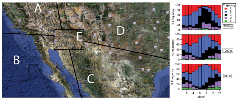
(left) Terrain map of the U.S. Southwest with the solid boxed region representing the area of interest in this study. The various sectors represented by letters correspond to different air mass source regions examined with HySplit back trajectories (see Figure 1, right), where the boxed region “E” signifies trajectories that spent a significant amount of time in the southern Arizona region. (right) Relative frequency of five day air mass back trajectories passing through the five marked sectors. The three graphs correspond to the three different ending altitudes (500, 1000, 3000 m AGL) in southern Arizona (32.12°N, −110.92°W).
2.2. Remote Sensing Data
Aerosol data were obtained from a variety of satellite remote sensors for the area bounded by the following coordinate range: 31°N, 33°N; −110°W, −112°W. Daily level 3 data were obtained from the Moderate Resolution Imaging Spectroradiometer (MODIS), Ozone Monitoring Instrument (OMI), Total Ozone Mapping Spectrometer (TOMS), and the Multiangle Imaging Spectroradiometer (MISR). AQUA MODIS data include the daily 1° gridded Deep Blue aerosol optical depth (AOD; 0.55 μm) [Hsu et al., 2004] and the 0.47/0.66 μm Ångstrom exponent between 2002 and 2009. The Deep Blue algorithm is suitable for desert regions because it is sensitive to particles over bright surfaces [Hsu et al., 2004], with AODs being within 20–30% of those measured by Sun photometers [Hsu et al., 2006]. Although not shown, monthly trends in the AOD (0.55 μm) and Ångstrom exponent (0.47/0.66 μm) from TERRA MODIS between February 2000 and December 2009 qualitatively resemble those of the AQUA Deep Blue AOD and Ångstrom exponent. AOD measurements (0.555 μm) between 2000 and 2009 were also obtained from MISR [Diner et al., 1998] at a resolution of 0.5° × 0.5°. Ultraviolet aerosol index (UV AI) data beginning in 1978 were provided by the TOMS (1° × 1.25°) and OMI (1° × 1°) sensors as a measurement of absorbing aerosols [Torres et al., 1998], which are predominantly composed of dust and smoke. A minimum UV AI threshold of 0.5 is applied in this study to account for instrumental uncertainties [Hsu et al., 1999]. Approximately 72% of the daily data available since 2000 exceeded this threshold.
The limitations associated with using satellite remote sensing data over land, mainly owing to problems with land surfaces, retrieval techniques, and cloud contamination, are well-documented elsewhere [Remer et al., 2005, 2008; Zhang and Reid, 2006, 2010; Levy et al., 2010]. To account for cloud contamination over land, remotely sensed aerosol data are only used when the MODIS cloud fraction (1° daily gridded product, MYD08_D3/MOD08_D3, Collection 5.1) is less than 70%. We further note that the aim of using these remote sensing data sets is to examine relative differences in retrieved parameters at a monthly resolution for intercomparison with other data sets described in sections 2.3 and 2.4.
2.3. Goddard Chemistry Aerosol Radiation and Transport (GOCART) Model
Daily simulations of the total optical depth (0.55 μm) associated with various aerosol components (total aerosol, coarse aerosol, fine aerosol, sulfate, dust, sea salt, organic carbon, and black carbon) were provided by the GOCART model [Chin et al., 2002]. Model results at a resolution of 2° × 2.5° longitude (within the spatial domain of 30°N, 34°N; −110°W, −112.5°W) were examined in this work.
2.4. Ground-Based Observations
2.4.1. Mt. Lemmon Observatory
A decade-long (1992–2002) measurement campaign at the University of Arizona High-Altitude Laboratory (32.26°N, −110.46°W, 2791 m ASL) on top of Mt. Lemmon, a “sky island” site used in several past studies (Table 1), provided monthly averaged measurements of aerosol composition. Extensive details of the experimental methods and measurements of aerosol and gaseous species are summarized by Matichuk et al. [2006]. Since the period of overlap with the majority of the satellite and ground-based aerosol data considered is between 2000 and 2002, only data from that period are reported. It is noted that the qualitative monthly trends for 2000–2002 are the same as for the period between 1992 and 2002. The aerosol-sampling system (Dp,50 = 2 μm) is summarized by Ohta et al. [1996]. Soluble ions were extracted from Teflon filters (Millipore Fluoropore 47 mm, 0.45 μm pore size). Quartz fiber filters (Pallflex, 2500QAO-UP, 47 mm) were used for measurements of organic carbon (OC) and elemental carbon (EC). Total aerosol mass was obtained using nylon filters (Millipore Nylon, 47 mm, 0.45 μm pore size).
2.4.2. EPA IMPROVE
Aerosol composition measurements from the Inter-agency Monitoring of Protected Visual Environments (IMPROVE) network of filter samplers [Malm et al., 1994; http://views.cira.colostate.edu/web/] were obtained for seven ground stations in Arizona (Figure 2). Monthly averaged data between 2000 and 2009 are reported, while data extending back to 1988 are also used from some sites (Tonto National Monument, Chiricahua National Monument, Saguaro National Monument) for long-term seasonal data trend analysis. Data from Queen Valley/Phoenix, Saguaro West, and Organ Pipe are only available since 2001, 2002, and 2003, respectively. The IMPROVE network of stations consists of filter samplers that collect daily aerosol samples usually on every third day. These samples are then analyzed for ions, metals, and both OC and EC. Sampling protocols and additional details are provided elsewhere (http://vista.cira.colostate.edu/improve/Publications/SOPs/UCDavis_SOPs/IMPROVE_SOPs.htm). The following equation is used to quantify fine soil concentrations [e.g., Malm et al., 2004]:
| (1) |
Figure 2.

Geographic location of the ground-based aerosol and meteorology measurements, with station altitudes above sea level reported in parentheses. The dashed box corresponds to the area over which the satellite data shown in Figure 6 and discussed in section 4.2 were collected.
Nitrate trend analyses are carried out starting in 2000 [http://vista.cira.colostate.edu/improve/Data/QA_QC/Advisory/da0002/da0002_WinterNO3.pdf], and all analyses including EC are carried out separately for the period before and after 2004 to account for a change in the thermal optical reflectance (TOR) analyzer used for sample analysis.
2.4.3. Aerosol Robotic Network (AERONET)
The AERONET measurements used in this study were conducted on top of the Meinel Building on the campus of the University of Arizona in Tucson (32.23°N, −110.95°W; 779 m ASL). Measurements at this site are available for the years 2000, 2001, and 2004–2006. Data are reported for AOD (0.50 μm), 0.50/0.87 μm Ångstrom exponent, and water vapor.
2.4.4. Meteorology
Meteorological data were obtained from three selected ground-based stations shown in Figure 2 (Wilcox, Tucson, and Maricopa) in the Arizona Meteorological Network (http://ag.arizona.edu/azmet/). Ambient temperature, soil temperature (2 inches below surface), relative humidity (RH), solar radiation, wind speed, and precipitation measurements between 2000 and 2009 are used.
3. Study Region Topography, Meteorology, and Fire Activity
The region under investigation is outlined in Figures 1–2 and includes the Sonoran Desert in the lower elevations of Arizona and mountain ranges in the southeastern part, including the Chiricahua Mountains in which one of the EPA IMPROVE sites is located. A major mountain range, including the Mogollon Rim, runs diagonally in a northwestern direction. Major topographical features in the vicinity of Tucson include the Santa Catalina Mountains to the north (highest point: Mt. Lemmon), Rincon Mountains to the east, Tucson Mountains to the west, Tortolita Mountains to the northwest, and the Santa Rita Mountains to the south. Southern Arizona is characterized by diverse types of vegetation: desert areas are covered with shrubs (e.g., creosote bush) and small trees such as palo verde, mesquite, and acacia; higher altitude sites such as Mt. Lemmon contain pines, junipers, oaks and firs; lower level metropolitan areas such as Tucson have considerable amounts of leaf biomass [Comrie and Diem, 1998] owing to native species (e.g., palo verde and creosote bush) and also more exotic species such as eucalyptus [Diem, 2000].
Southern Arizona is characterized by an arid climate with hot summers and generally mild winters. Decadal-averaged meteorological data from three representative low-altitude sites in southern Arizona are reported in Figure 3 (locations shown in Figure 2). The annual mean temperatures are 15.0° ± 2.8°C (Wilcox, southeastern Arizona), 20.8° ± 2.9°C (Maricopa, southwestern Arizona), and 20.2° ± 3.1°C (Tucson, southeast/central Arizona). The monthly temperature curve is characterized by a minimum in December and a maximum in July. Soil temperature closely mimics the monthly trend of ambient air temperature, reaching maximum levels in the summer months between May and July. Although not shown in Figure 3, solar radiation at all three sites peaks either in May or June. As expected, RH exhibits nearly the opposite monthly behavior in comparison with temperature, with the exception of major enhancements between July and August owing to the arrival of monsoon moisture. Average RH is less than 35% in the driest months of May and June. Although the monthly averaged wind speeds are below the threshold wind velocities needed for dust emission events (>5–15 m s−1) over a range of surfaces (e.g., mine tailings, disturbed desert, abandoned land, scrub desert) [Leinen and Sarnthein, 1989], wind speeds during episodic events frequently exceed these threshold velocities in southern Arizona. This is especially the case between April and July in addition to gust fronts associated with deep convective cells during the monsoon season (July–September).
Figure 3.

Monthly summary of daily averaged meteorological data at three southern Arizona sites (see locations in Figure 2) between 2000 and 2009. The x axis (1–12) represents January–December.
Precipitation in southern Arizona falls in two major modes. The first is between November and March as a result of Pacific Ocean frontal storms. The second, being a crucial climatic feature of southern Arizona, is the summertime monsoon rainfall that typically occurs between July and September, where high-level moisture is transported predominantly from the Gulf of Mexico and from the eastern tropical Pacific Ocean and Gulf of California area at lower altitudes [Adams and Comrie, 1997; Higgins et al., 1997]. Moisture from these two sources mixes over the Sierra Madre Occidental region of Mexico prior to being transported north toward the United States. Precipitation data in Figure 3 show the overwhelming importance of these storms relative to all other months. The total annual precipitation (average over 2000–2009) at the examined sites amounts to 257 mm (Wilcox), 266 mm (Tucson), and 110 mm (Maricopa), with the majority of the accumulation usually during the summer months.
Of critical importance to the study of temporal trends in aerosol concentrations are mixing layer heights in the region. Figure 4 summarizes the average mixing layer height for Tucson, Maricopa, and Wilcox using output data for 2009 from a Weather and Research Forecasting (WRF) model run using the Yonsei University boundary layer scheme on a 36 km grid [Hu et al., 2010]. The highest average mixing layer heights (~1.4–1.5 km AGL) occur in July at all three locations, while the lowest average heights occur in January (~300–400 m AGL). The afternoon mixing layer heights at 1500 local time, representative of daily maximum heights, exhibit a different monthly trend with a peak near 3.5 km AGL in Tucson and Wilcox during August. The minimum mixing layer heights (0600 local time) are usually between 50 and 150 m AGL. These results indicate that there is considerable dilution of aerosol concentrations in the summer months in comparison with winters, because boundary layers are deeper on average by a factor of three to five. Figure 4 also shows representative vertical temperature profiles for Tucson (32.23°N; −110.96°W) obtained from soundings (http://weather.uwyo.edu/upperair/sounding.html; University of Wyoming) during different seasons and at two times of the day (0500 and 1700 local time) for the year 2001. A low-level temperature inversion (~1 km ASL) is evident during the early morning and is most pronounced during the winter months, promoting the accumulation of pollutants near the surface. (Note that station altitude is at 751 m ASL.) Afternoon data show that the boundary layer is expectedly deeper owing to higher ambient temperatures and convective activity with an average inversion height between 1.5 and 3 km ASL. During the monsoon, the mixing height can extend to the tropopause because of intense convection.
Figure 4.

(a–c) Average monthly mixing layer heights in Tucson, Maricopa, and Wilcox (see Figure 2 for locations and Figure 3 for respective meteorological data) for the year 2009. The markers correspond to the average mixing layer height over all hours in a given month, and the whiskers denote the average mixing heights at 1500 (representative of afternoon maximum) and 0600 (representative of the morning minimum). (d–g) Monthly average vertical temperature profiles at 0000Z (1700 local time) and 1200Z (0500 local time) for four months in Tucson (32.23°N; −110.96W°, station at 751 m ASL) based on 2001 sounding data from the University of Wyoming (http://weather.uwyo.edu/upperair/sounding.html). A representative dry adiabatic sounding is included as a guide.
Wildfires play a large role in the region seasonally. The spatiotemporal distribution of detected fires, as identified by Terra MODIS, is shown in Figure 5 for the period 2000–2009 (courtesy of http://firefly.geog.umd.edu/firemap/; Justice et al. [2002], Giglio et al. [2003], Davies et al. [2009]). Fires are widely distributed across southern Arizona with the highest incidence of fires detected in the mountainous and forested terrain of the Mogollon Rim in the northeastern section of the study region. Fire maps are also shown for different months for a representative year (2004), illustrating the dependence of fires on the time of year. June and the early half of July exhibit the highest incidence of fires in the mountainous areas. The onset of monsoon precipitation (mid-July) substantially reduces the numbers of fires through August. The fall (SON) and spring months (MAM) have comparable amounts of fires, while the winter months, with episodic rain and snow at higher elevations, are characterized by the fewest detected fires.
Figure 5.

Spatiotemporal distribution of detected fires in southern Arizona as identified by Terra MODIS (courtesy of http://firefly.geog.umd.edu/firemap/; Justice et al. [2002], Giglio et al. [2003], Davies et al. [2009]). Data are shown for cumulative fires (top left) between 2000 and 2009 and during specific months for a representative year (other panels).
4. Results and Discussion
4.1. Back Trajectory Analysis
Figure 1 summarizes the relative frequency of trajectories transported through the five different sectors at three ending altitudes (500, 1000, 3000 m AGL). The most common trajectory at all altitudes on an annual basis was trajectory B (46%/42%/34% at 500/1000/3000 m), corresponding to marine-influenced aerosol transported over dust-rich areas in the southernmost parts of the United States and in Baja California. The second most common trajectory at each altitude was trajectory A (22%/26%/27% at 500/1000/3000 m), followed by trajectory C (16%/17%/24% at 500/1000/3000 m). Trajectories D (11%/11%/13% at 500/1000/3000 m) and E (≤5%) were the least common.
The relative frequencies of the trajectories for ending altitudes of 500 m and 1000 m were similar to each other, while trajectories ending at 3000 m more frequently originate in sectors C and D between July and September. The back trajectory findings are consistent with monsoon moisture (July–September) originating in the Gulf of Mexico at high altitudes and the Gulf of California at lower altitudes; it is evident that trajectory C becomes most dominant in these months at 3000 m, while trajectory B is most frequent at the lower altitudes.
4.2. Remote Sensing Data
Figures 6a–6f summarize monthly averaged remote sensing data for aerosol composition, AOD, Ångstrom exponent, and UV AI for a large area surrounding Tucson (31°N, 33°N; −110°W, −112°W). Although not shown, an analogous analysis of satellite data for a comparable area containing Phoenix (33°N, 34°N; −111°W, −113°W) shows nearly identical monthly trends for all parameters in Figure 6. Table S1 reports average values of the retrieved parameters as a function of air mass origin (see Figure 1) for different seasons and on an annual basis.1 AOD from both MISR and MODIS is highest between the months of May and August. Water vapor measurements at the AERONET station show a dramatic enhancement in moisture between June and October, which is at least partly responsible for higher AOD values owing to aerosol hygroscopic growth (i.e., water uptake by particles) and enhanced aerosolladen water promoting production of particulate mass via multiphase processes. Monthly trends in UV AI differ from those of AOD, in that its values are typically the highest between April and June and decrease to a minimum in August. The AERONET and MODIS Ångstrom exponents fall to a minimum in the months of April through June, indicating that larger particles (e.g., dust) are most abundant during this time of the year. This is further supported by meteorological conditions which promote wind-blown dust events during these months (high temperature and wind speed, low precipitation). Long-range transport of Asian dust may play an additional role. Unlike AOD, UV AI does not decrease after August, but tends to slightly increase; a subsequent discussion of aerosol composition (Section 4.4) points to a contribution from fine soil between August and November.
Figure 6.

Average monthly trends for different aerosol parameters: (a) MODIS Ångstrom exponent; (b) MISR AOD (0.555 μm) and MODIS Deep Blue AOD (0.55 μm); (c) TOMS and OMI UV aerosol index; (d–f) AERONET data from Tucson; (g–i) GOCART data for the optical depth (0.55 μm) associated with different classes of aerosol types.
Previous surface-based measurements in Tucson (1975–1977; King et al. [1980]) showed that peak AOD levels occurred in July and August, which is consistent with the results presented in Figure 6. Surface-based remote sensing measurements in the town of Tombstone (31.38°N, −110.08°W, 1408 m ASL) in 1997 [Pinker et al., 2004] showed that peak AOD values occurred slightly later, in the months of July through September, and reached lowest values during the winter. The Ångstrom exponent in their study was highest between August and October and lowest in May (no measurements available in April), which is consistent with the remote sensing data in Figure 6. The next few sections will use models and ground measurements of aerosol composition to explain the trends and differences observed in these remote sensing data sets.
4.3. GOCART Data
Figures 6g–6i summarize GOCART monthly trends for AOD associated with various aerosol species. Monthly trends of coarse-mode AOD are nearly identical to those of dust, with peak levels in April and May and lowest levels in August. Fine-mode AOD peaks in July and is generally the highest between April and August, while reaching a minimum in the month of December (Figure 6i). Coarse- and fine-mode dust exhibit identical monthly trends with the latter typically being a third the value of coarse-dust AOD (Figure 6h). Fine-mode AOD contributes more to total AOD than coarse-mode AOD during all months. It is only between April and May that the coarse-aerosol AOD approaches the values of fine-aerosol AOD. This is caused by dust, which is consistent with the lowest observed Ångstrom exponents during this time. The monthly trends in AERONET and satellite-retrieved AODs differ from those of GOCART total AOD, because they remain high during the summer until August, whereas the GOCART AOD begins to decrease in May. This discrepancy is possibly due to GOCART underestimating AOD enhancements because of wildfires in June and July and increasing water vapor during the monsoon season.
The GOCART results point to the importance of non-dust aerosol outside the months of March through June. Important components of fine aerosol, especially during the monsoon season, include organic carbon (OC) and sulfate. Black carbon (BC) is predicted to be most abundant between April and June, similar to dust; however, dust is more important to the satellite-retrieved UV AI based on the predicted low optical depths associated with BC relative to dust (subsequent discussion of ground-based aerosol data will confirm this). Fires influence the region, but these events are not sufficiently persistent to compete with atmospheric dust loadings on the monthly time scales examined in this study, especially since UV AI decreases when fires typically are most influential in the region (June–July; Figure 6). Sea salt is shown to be the smallest contributor to the AOD in the southern Arizona region in all months. It is highest between December and March when air mass trajectories originating over the Pacific Ocean at high altitudes are most frequent. The predicted low levels of sea salt can be attributed to their large size, their hygroscopic nature, and the resulting short average lifetime in the atmosphere [Chin et al., 2002], which minimizes transport to southern Arizona. Malm and Sisler [2000] previously showed very steep decreasing gradients in sodium (Na+; a component of sea salt) between coastal U.S. regions and areas just a few hundred kilometers inland. Furthermore, Chow and Watson [2001] showed that the contribution of sea salt to PM10 was less than 4% in their measurements at a site near the U.S.-Mexico border by Imperial Valley and Mexicali Valley, which is closer to the ocean than southern Arizona.
4.4. Ground-Based Aerosol Composition Data
Ground-based measurements at the summit of Mt. Lemmon and various other ground sites across southern Arizona offer another data set to compare with satellite and GOCART data, and to build a more detailed chemical climatology of the regional aerosol. Figure 7 shows monthly averaged chemical measurements common to all examined measurement sites, while Figure 8 shows decadal averages of mass fractions of major aerosol constituents at the seven EPA IMPROVE sites. Table S1 summarizes the average values of aerosol composition measurements as a function of air mass origin. As the back trajectories were examined for Tucson, IMPROVE measurements from the Saguaro National Monument are used for Table S1 because this site is closest to the endpoint of trajectory analysis. A brief description of the measurement sites follows.
Figure 7.

Monthly averages of aerosol composition for Mt. Lemmon and the EPA IMPROVE measurement sites shown in Figure 2. Note that the y axis ranges differ between stations for a given aerosol species. Values for the OC:EC ratio are unitless and are reported separately for the periods 2000–2004 and 2005–2009, since, after 2004, a new thermal optical reflectance (TOR) analyzer was used for IMPROVE carbon analysis.
Figure 8.
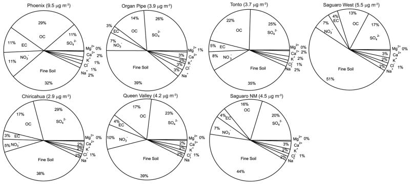
Average mass fractions of major PM2.5 constituents at seven EPA IMPROVE sites between 2000 and 2009 (some stations only have data starting after the year 2000; see section 2.4.2). The total mass concentrations above each pie chart correspond to the sum of the ten aerosol components shown.
4.4.1. Site Descriptions
The University of Arizona High-Altitude Laboratory at the summit of Mt. Lemmon (2791 m ASL) is a high-altitude site. Aerosol concentrations are therefore expected to be low, especially in the winter months when the mixing layer height is below the altitude of this site and urban pollution does not reach the summit. Multiple pollution sources can influence Mt. Lemmon including, most importantly, the city of Tucson (20 km southwest of Mt. Lemmon), followed by the village of Summerhaven about 3 km east of the laboratory (includes cabins and a small ski area), and Phoenix (approximately 140 km northwest of the laboratory). Measurements have confirmed that, during the wintertime with stronger temperature inversions, the sampled aerosol is largely representative of free tropospheric aerosol [Twomey, 1983; Philippin and Betterton, 1997; Shaw, 2007]. During the summer months (May–August) when there is strong convection, the sampled aerosol is strongly influenced by Tucson pollution, while there is minimal influence between the months of November–February. The months of March, April, September, and October are characterized by highly variable mixing heights, thereby allowing pollution to be transported to the summit by upslope winds.
Chiricahua National Monument (32.0089°N, −109.3891°W; 1570 m ASL) is a fairly remote vegetated site with the nearest major urban area being Tucson, which is approximately ~150 km to the west. The nearest major aerosol sources are the Wilcox playa and the Apache Power Plant, which are ~45 km to the west. Of all the sites examined, Chiricahua is the closest to the Chihuahuan Desert and other sources of dust near the borders of Mexico with New Mexico and Texas. The Phoenix site (33.5038°N, −112.0958°W; 338 m ASL) is centrally located within the metropolitan area and is the site most influenced by urban pollution. Two other sites that have a high potential to be influenced by the Phoenix urban plume are the Tonto National Monument (33.6494°N, −111.1088°W; 786 m ASL), which is approximately ~90 km to the east/northeast, and Queen Valley (33.2939°N, −111.2857°W; 658 m ASL), which is ~60 km to the east and is ~45 km south of the Tonto site. Organ Pipe (31.9506°N, −112.8016°W; 505 m ASL) is just north of the U.S.-Mexico border. Aside from nearby dust sources (e.g., Ajo mine immediately to the north), the nearest source of anthropogenic pollution is the town of Sonoita, Mexico, approximately 10 km to the southwest with ~10,000 inhabitants. Saguaro National Monument (32.1742°N, −110.7372°W; 933 m ASL) is located at the eastern end of the Tucson metropolitan area in the foothills of the Rincon Mountains, while the Saguaro West site (32.2486°N, −111.2178°W; 718 m ASL) is located near the western side of the Tucson metropolitan area. The two sites are separated by almost 50 km and are both influenced by the Tucson urban plume.
4.4.2. PM10 and PM2.5
Peak monthly PM10 concentrations range from as low as 16 μg m−3 in Chiricahua (May–June) to as high as 34 μg m−3 in Phoenix (May) (Figure 7). PM2.5 levels generally follow the same monthly trend as PM10, with the highest concentrations for both metrics typically confined to the corridor between Phoenix and Tucson, which includes the Phoenix, Saguaro West, and Queen Valley sites. The highest PM2.5 was observed in Phoenix (16.4 μg m−3, December) and the lowest at Mt. Lemmon (PM2.0 = 0.26 μg m−3, December; note that PM2.0 rather than PM2.5 was measured at Mt. Lemmon). As shown in Figure 8, PM2.5 is dominated by fine soil, followed by organic carbon, sulfate, and nitrate. The mass fractions of the major PM2.5 components vary across southern Arizona, with major differences being higher OC and EC in Phoenix and higher fine soil at the Tucson sites. The similarity in the monthly trends of PM10 and PM2.5 (r2 > 0.72 at all sites; n = 12) suggests that dust impacted total particulate concentrations in both the fine and coarse fractions. This is also reflected in the secondary peak in both PM10 and PM2.5 at the Tucson stations (Saguaro West and Saguaro National Monument) between October and November, which matches a similar peak in fine soil.
PM10 and PM2.5 reach their highest levels in the summertime (May–August) at all stations except Phoenix. The different monthly behavior of PM10 in Phoenix is associated with higher local emissions as a result of anthropogenic activity such as vehicles and fugitive and wind-blown dust from agricultural fields, roads, and construction activity. The highest PM10 and PM2.5 levels are observed in the winter when pollution from these activities accumulates in a shallow boundary layer (Figure 4). Contrary to the other IMPROVE sites, the Phoenix data suggest that aerosol sources that are more active during the summertime (e.g., photochemical production of aerosol species, dust emissions, fires, biogenic emissions) are not sufficiently strong to outweigh the effect of a deepening boundary layer and volatilization effects with regard to PM levels in the summer. It is further noted that Maricopa County, which includes Phoenix, is a PM10 nonattainment area (http://www.epa.gov/oaqps001/greenbk/pnp.html).
The higher-altitude sites (Chiricahua and Mt. Lemmon) expectedly exhibit lower PM concentrations than all other sites. While PM10 measurements are not available at Mt. Lemmon, the PM2.0 levels are the lowest among all sites owing to dilution with increasing altitude and the sampling of free tropospheric aerosol during the winter months. PM2.0 values reach their highest levels between June and August (2.56 ± 0.73 μg m−3) and drop to 0.45 ± 0.21 μg m−3 between November and February. Figure 4 shows that the average and maximum mixing layer heights in Tucson are highest between June and August, allowing the pollution from Tucson to reach the Mt. Lemmon Observatory. Thus, the Mt. Lemmon concentrations are governed to a large extent by mixing layer height at different times of the year (Figure 4).
4.4.3. Sulfate ( )
In the past, copper smelters in southern Arizona and Mexico were reported to be a major source of [Malm, 1992], but their widespread closure before the year 2000 suggests that other sources are probably more important since that time [Matichuk et al., 2006]. It will be shown subsequently that sulfate levels have indeed decreased across southern Arizona since before 2000 (Table 2 and section 4.5). Sulfate monthly trends are similar at all sites with maximum levels in the summer months between June and August, which is consistent with GOCART data. Sulfate contributes an average of 10%–30% to PM2.5 in the region (Figure 8). The absolute concentrations of are comparable among the measurement sites in southern Arizona, with slightly higher values in Phoenix and Organ Pipe. Interestingly, the highest monthly concentration is found at Organ Pipe (1.71 ± 0.82 μg m−3 in July) rather than in Phoenix, which is presumably due to nearby sources. The similarity in monthly trends among the various sites points to the importance of gas-to-particle conversion processes for sulfate production. The monsoon months exhibit an increase in RH and column water vapor (Figures 3 and 6), which suggests that aqueous-phase production of is an important process in this region. This is confirmed by the peak in solar radiation (May–June) preceding that of sulfate, indicating that photochemistry alone is insufficient to explain the summertime sulfate enhancements. The similarity in summertime concentrations between Mt. Lemmon and the lower level Tucson sites confirms that convection and lifting of the Tucson urban plume influences the sky-island site. Sulfate levels are dramatically lower in the winter months at Mt. Lemmon owing to a significantly reduced anthropogenic signature in the free tropospheric aerosol.
Table 2.
Linear Regression Trends (μg m−3 year−1 for Aerosol Species and year−1 for OC:EC Ratio) for the Following IMPROVE Stations Shown in Figure 2 With Respective Dates That Data Were Availablea
| DJF
|
|||||||||||||||
|---|---|---|---|---|---|---|---|---|---|---|---|---|---|---|---|
| Chiricahua NM
|
Tonto NM
|
Phoenix
|
Saguaro NM
|
Organ Pipe
|
Queen Valley
|
Saguaro West
|
|||||||||
| Slope | r2 | Slope | r2 | Slope | r2 | Slope | r2 | Slope | r2 | Slope | r2 | Slope | r2 | ||
| PM10 | 0.028 (0.074) | 0.01 | −0.156 (0.066) | 0.23 | −2.083 (1.460) | 0.25 | −0.106 (0.102) | 0.10 | −0.256 (0.492) | 0.05 | −0.342 (0.617) | 0.05 | −0.525 (0.808) | 0.07 | |
| PM2.5 | −0.034 (0.018) | 0.15 | −0.092 (0.015) | 0.67 | −0.704 (0.450) | 0.29 | −0.073 (0.031) | 0.31 | −0.218 (0.081) | 0.59 | −0.342 (0.617) | 0.05 | −0.525 (0.808) | 0.07 | |
| Fine Soil | 0.025 (0.009) | 0.25 | 0.019 (0.010) | 0.16 | −0.106 (0.268) | 0.03 | 0.028 (0.025) | 0.12 | −0.065 (0.082) | 0.11 | −0.187 (0.110) | 0.33 | −0.078 (0.203) | 0.02 | |
| OC | −0.009 (0.004) | 0.18 | −0.021 (0.006) | 0.39 | −0.373 (0.090) | 0.74 | −0.014 (0.004) | 0.53 | −0.068 (0.011) | 0.89 | −0.047 (0.083) | 0.05 | −0.013 (0.174) | 0.00 | |
| EC (1988–2004) | −0.003 (0.001) | 0.24 | −0.006 (0.002) | 0.40 | - | - | −0.007 (0.002) | 0.75 | - | - | −0.042 (0.006) | 0.90 | −0.035 (0.013) | 0.56 | |
| EC (2005–2009) | −0.016 (0.005) | 0.79 | −0.029 (0.012) | 0.74 | −0.180 (0.125) | 0.41 | −0.025 (0.015) | 0.49 | −0.022 (0.010) | 0.70 | - | - | 0.000 (0.014) | 0.00 | |
| OC:EC (1988–2004) | 0.038 (0.038) | 0.06 | 0.012 (0.034) | 0.01 | - | - | 0.029 (0.011) | 0.56 | - | - | −0.018 (0.016) | 0.32 | −0.028 (0.018) | 0.56 | |
| OC:EC (2005–2009) | 0.161 (0.169) | 0.23 | 0.422 (0.120) | 0.86 | −0.004 (0.039) | 0.00 | 0.167 (0.059) | 0.73 | 0.097 (0.181) | 0.12 | - | - | −0.115 (0.157) | 0.21 | |
|
|
−0.027 (0.004) | 0.78 | −0.033 (0.005) | 0.79 | −0.040 (0.016) | 0.52 | −0.036 (0.004) | 0.94 | −0.079 (0.026) | 0.66 | −0.032 (0.153) | 0.01 | −0.014 (0.006) | 0.76 | |
|
|
−0.005 (0.002) | 0.03 | −0.001 (0.003) | 0.00 | −0.112 (0.091) | 0.20 | −0.004 (0.006) | 0.05 | 0.014 (0.004) | 0.71 | −0.035 (0.010) | 0.65 | −0.021 (0.008) | 0.56 | |
| MAM
|
|||||||||||||||
|---|---|---|---|---|---|---|---|---|---|---|---|---|---|---|---|
| Chiricahua NM
|
Tonto NM
|
Phoenix
|
Saguaro NM
|
Organ Pipe
|
Queen Valley
|
Saguaro West
|
|||||||||
| Slope | r2 | Slope | r2 | Slope | r2 | Slope | r2 | Slope | r2 | Slope | r2 | Slope | r2 | ||
| PM10 | 0.030 (0.081) | 0.01 | −0.052 (0.071) | 0.03 | −0.473 (0.670) | 0.07 | −0.128 (0.099) | 0.15 | 0.201 (0.325) | 0.07 | 0.109 (0.337) | 0.01 | 0.132 (0.466) | 0.01 | |
| PM2.5 | 0.030 (0.081) | 0.01 | −0.052 (0.071) | 0.03 | −0.473 (0.670) | 0.07 | −0.128 (0.099) | 0.15 | 0.201 (0.325) | 0.07 | 0.109 (0.337) | 0.01 | 0.132 (0.466) | 0.01 | |
| Fine Soil | −0.013 (0.021) | 0.02 | −0.012 (0.028) | 0.01 | −0.111 (0.073) | 0.25 | 0.008 (0.043) | 0.00 | −0.091 (0.186) | 0.05 | −0.017 (0.101) | 0.00 | 0.064 (0.207) | 0.02 | |
| OC | 0.032 (0.013) | 0.25 | 0.053 (0.015) | 0.38 | 0.033 (0.060) | 0.04 | 0.052 (0.030) | 0.24 | 0.104 (0.097) | 0.19 | 0.078 (0.066) | 0.17 | 0.153 (0.129) | 0.19 | |
| EC (1988–2004) | −0.014 (0.005) | 0.30 | −0.014 (0.006) | 0.24 | −0.091 (0.034) | 0.51 | −0.008 (0.005) | 0.22 | −0.085 (0.025) | 0.70 | −0.029 (0.020) | 0.22 | −0.027 (0.018) | 0.28 | |
| EC (2005–2009) | −0.002 (0.001) | 0.14 | −0.003 (0.002) | 0.14 | −0.024 (0.041) | 0.15 | −0.007 (0.001) | 0.81 | - | - | - | - | - | - | |
| OC:EC (1988–2004) | −0.012 (0.002) | 0.95 | −0.010 (0.008) | 0.12 | −0.068 (0.014) | 0.88 | −0.021 (0.003) | 0.94 | −0.002 (0.007) | 0.04 | −0.027 (0.010) | 0.71 | −0.013 (0.003) | 0.85 | |
| OC:EC (2005–2009) | −0.005 (0.049) | 0.00 | 0.045 (0.058) | 0.04 | 0.227 (0.308) | 0.21 | 0.121 (0.026) | 0.81 | - | - | - | - | - | - | |
|
|
0.459 (0.216) | 0.60 | 0.198 (0.228) | 0.20 | 0.143 (0.150) | 0.23 | 0.267 (0.186) | 0.41 | 0.097 (0.181) | 0.12 | 0.442 (0.341) | 0.36 | 0.108 (0.140) | 0.17 | |
|
|
−0.009 (0.005) | 0.17 | −0.003 (0.004) | 0.04 | −0.005 (0.013) | 0.02 | −0.010 (0.004) | 0.43 | −0.072 (0.021) | 0.69 | 0.003 (0.011) | 0.01 | −0.001 (0.012) | 0.00 | |
| JJA
|
|||||||||||||||
|---|---|---|---|---|---|---|---|---|---|---|---|---|---|---|---|
| Chiricahua NM
|
Tonto NM
|
Phoenix
|
Saguaro NM
|
Organ Pipe
|
Queen Valley
|
Saguaro West
|
|||||||||
| Slope | r2 | Slope | r2 | Slope | r2 | Slope | r2 | Slope | r2 | Slope | r2 | Slope | r2 | ||
| PM10 | −0.054 (0.080) | 0.02 | −0.039 (0.090) | 0.01 | −0.904 (0.712) | 0.19 | −0.176 (0.103) | 0.21 | 0.150 (0.355) | 0.03 | −0.253 (0.547) | 0.03 | −1.389 (0.599) | 0.47 | |
| PM2.5 | −0.083 (0.032) | 0.25 | −0.024 (0.030) | −0.03 | −0.214 (0.162) | 0.20 | −0.051 (0.053) | 0.07 | −0.024 (0.117) | 0.01 | −0.144 (0.140) | 0.13 | −0.658 (0.351) | 0.37 | |
| Fine Soil | 0.022 (0.013) | 0.13 | 0.015 (0.012) | 0.07 | 0.055 (0.095) | 0.04 | 0.037 (0.027) | 0.14 | 0.079 (0.089) | 0.14 | 0.014 (0.050) | 0.01 | −0.330 (0.141) | 0.48 | |
| OC | −0.018 (0.007) | 0.28 | −0.011 (0.008) | 0.09 | −0.103 (0.031) | 0.61 | −0.006 (0.011) | 0.02 | −0.085 (0.025) | 0.84 | −0.036 (0.027) | 0.21 | −0.058 (0.024) | 0.48 | |
| EC (1988–2004) | −0.004 (0.001) | 0.31 | −0.004 (0.002) | 0.22 | −0.007 (0.020) | 0.06 | −0.004 (0.003) | 0.20 | - | - | - | - | - | - | |
| EC (2005–2009) | −0.012 (0.005) | 0.66 | −0.028 (0.013) | 0.62 | −0.085 (0.017) | 0.90 | −0.026 (0.000) | 0.98 | −0.008 (0.006) | 0.33 | −0.027 (0.009) | 0.73 | −0.018 (0.002) | 0.94 | |
| OC:EC (1988–2004) | 0.107 (0.055) | 0.20 | 0.092 (0.052) | 0.17 | 0.066 (0.246) | 0.04 | 0.109 (0.035) | 0.62 | - | - | - | - | - | - | |
| OC:EC (2005–2009) | 0.706 (0.993) | 0.14 | 0.223 (0.344) | 0.12 | 0.207 (0.095) | 0.61 | 0.136 (0.265) | 0.08 | −0.229 (0.306) | 0.22 | 0.123 (0.261) | 0.07 | 0.225 (0.225) | 0.25 | |
|
|
−0.033 (0.007) | 0.51 | −0.018 (0.006) | 0.33 | −0.025 (0.022) | 0.16 | −0.023 (0.007) | 0.50 | −0.054 (0.033) | 0.34 | −0.029 (0.023) | 0.18 | −0.049 (0.027) | 0.36 | |
|
|
0.000 (0.001) | 0.01 | 0.002 (0.001) | 0.06 | 0.000 (0.006) | 0.00 | −0.001 (0.002) | 0.01 | 0.006 (0.006) | 0.15 | −0.006 (0.006) | 0.12 | −0.009 (0.007) | 0.22 | |
| SON
|
|||||||||||||||
|---|---|---|---|---|---|---|---|---|---|---|---|---|---|---|---|
| Chiricahua NM
|
Tonto NM
|
Phoenix
|
Saguaro NM
|
Organ Pipe
|
Queen Valley
|
Saguaro West
|
|||||||||
| Slope | r2 | Slope | r2 | Slope | r2 | Slope | r2 | Slope | r2 | Slope | r2 | Slope | r2 | ||
| PM10 | −0.073 (0.053) | 0.09 | −0.146 (0.085) | 0.01 | −1.166 (0.574) | 0.37 | −0.108 (0.085) | 0.13 | 0.605 (0.373) | 0.34 | −0.321 (0.179) | 0.32 | −0.316 (0.526) | 0.06 | |
| PM2.5 | −0.046 (0.016) | 0.29 | −0.084 (0.031) | 0.27 | −0.343 (0.145) | 0.45 | −0.026 (0.052) | 0.02 | 0.169 (0.113) | 0.31 | −0.114 (0.077) | 0.24 | −0.218 (0.213) | 0.15 | |
| Fine Soil | 0.012 (0.008) | 0.11 | 0.018 (0.011) | 0.11 | −0.080 (0.077) | 0.13 | 0.054 (0.037) | 0.17 | 0.140 (0.054) | 0.57 | −0.027 (0.043) | 0.05 | −0.128 (0.175) | 0.08 | |
| OC | −0.018 (0.006) | 0.32 | −0.027 (0.011) | 0.24 | −0.171 (0.057) | 0.56 | −0.010 (0.006) | 0.23 | −0.065 (0.027) | 0.54 | −0.034 (0.020) | 0.29 | −0.046 (0.021) | 0.45 | |
| EC (1988–2004) | −0.004 (0.002) | 0.25 | −0.006 (0.003) | 0.21 | 0.078 (0.031) | 0.76 | −0.007 (0.003) | 0.50 | - | - | - | - | - | - | |
| EC (2005–2009) | −0.015 (0.003) | 0.92 | −0.017 (0.005) | 0.79 | −0.143 (0.060) | 0.65 | −0.030 (0.002) | 0.98 | −0.012 (0.005) | 0.71 | −0.019 (0.012) | 0.47 | −0.031 (0.005) | 0.94 | |
| OC:EC (1988–2004) | 0.023 (0.035) | 0.03 | 0.033 (0.028) | 0.09 | −0.243 (0.273) | 0.28 | 0.053 (0.028) | 0.37 | - | - | - | - | - | - | |
| OC:EC (2005–2009) | 0.324 (0.174) | 0.54 | 0.397 (0.033) | 0.98 | 0.180 (0.061) | 0.74 | 0.259 (0.096) | 0.71 | 0.186 (0.123) | 0.54 | 0.217 (0.099) | 0.62 | 0.141 (0.122) | 0.30 | |
|
|
−0.025 (0.007) | 0.37 | −0.020 (0.005) | 0.42 | −0.042 (0.022) | 0.35 | −0.026 (0.007) | 0.57 | 0.013 (0.851) | 0.01 | −0.022 (0.024) | 0.11 | −0.018 (0.029) | 0.06 | |
|
|
0.000 (0.001) | 0.01 | 0.000 (0.003) | 0.00 | −0.043 (0.028) | 0.24 | 0.003 (0.004) | 0.06 | −0.027 (0.015) | 0.41 | −0.022 (0.023) | 0.12 | −0.024 (0.013) | 0.37 | |
Chiricahua National Monument (1988–2009), Tonto National Monument (1988–2009), Saguaro National Monument (1989–1992, 2000–2009), Saguaro West (2002–2009), Phoenix (2001–2009), Organ Pipe (2003–2009), and Queen Valley (2001–2009). The numbers in parentheses correspond to standard deviations of the slopes.
4.4.4. Organic Carbon (OC)
Particulate organics originate from direct emission (e.g., dust and primary biological aerosol particles such as pollen, fungi, and bacteria) and from secondary gas-to-particle conversion processes as a result of volatile organic compound (VOC) emissions. A number of recent studies examined the nature of OC at various southwestern U.S. IMPROVE sites [Bench et al., 2007; Schichtel et al., 2008; Holden et al., 2011] with an aim to identify the major sources of OC at urban and rural sites. At Tonto and Phoenix, Holden et al. [2011] showed that the OC produced from the combination of primary biomass combustion, fungal spore emissions, and secondary OC formation from isoprene oxidation was substantially less than the total contemporary carbon. They suggested that other contributions could have their origin in secondary organic aerosol (SOA) formation from other VOCs, meat cooking, plant debris, biodiesel combustion, and humic-like substances (HULIS). Schichtel et al. [2008] observed contemporary carbon fractions of ~50% at urban sites and enhanced levels (82%–100%) at rural sites suggesting that biogenic carbon may be less important in areas such as Phoenix compared with Tonto.
Our results show that OC exhibits remarkably different behavior in Phoenix in comparison with the other sites. OC is most abundant in Phoenix (up to 6.2 ± 4.5 μg m−3 in December) with a monthly trend closely mimicking that of EC, pointing to the important influence of anthropogenic emissions. The other sites show OC peaks between May and July. The next most urban-influenced site (Saguaro West) exhibits a second mode in OC mass in the winter months that is comparable in magnitude to the summertime OC peak (~0.8 μg m−3), with the former owing to anthropogenic emissions. Interestingly, the OC levels in May (~0.75–0.85 μg m−3) and August (~0.60–0.72 μg m−3) are nearly the same for the Mt. Lemmon site and the two lower-altitude sites in Tucson. This suggests that local sources of OC (e.g., fires, fossil fuel burning, and dust) and transported aerosols may contribute to these increased high-altitude levels. As will be shown in Figure 7, the other chemical tracers showing enhanced concentrations in May and August at Mt. Lemmon are EC (tracer for biomass and fossil fuel combustion) and chloride (a crustal tracer).
Annually, OC accounts for between 13% and 29% of the major PM2.5 constituents across southern Arizona (Figure 8). To convert OC mass to total organic aerosol mass, a correction factor typically ranging between 1.4 and 2.1 is applied to estimate the average molecular weight per carbon weight for the organic aerosol [Turpin and Lim, 2001]. As a result, the total organic mass in Phoenix is estimated to be larger than that of the inorganic components, while more comparable levels of organic and inorganic species are observed at the other sites.
4.4.5. Elemental Carbon (EC)
Major sources for EC are biomass burning and fossil fuel combustion [Bond et al., 2004]. EC is most abundant in the winter months in southern Arizona owing to lower mixing layer heights at this time of the year (Figure 4) and the lack of a secondary production mechanism promoted by solar radiation and elevated RH. Residential heating may be an additional source of EC that is absent during other times of the year. The more remote areas such as Chiricahua and Mt. Lemmon do not exhibit a clear increase in EC during the winter. This is because these sites are above the average mixing layer height at that time of the year and are less influenced by anthropogenic activity. Mt. Lemmon EC values exhibit a dramatic enhancement between May and August, similar to OC, owing to the influence of the Tucson urban plume and biomass burning during those months. However, in May and August, the Mt. Lemmon EC levels exceed those at both lower-altitude Tucson stations presumably beacause of a combination of local vehicular emissions and biomass burning plumes. Concentrations of EC are relatively similar in magnitude across the network of sites with the exception of Phoenix, which exhibits significantly higher levels. The satellite-retrieved UV AI corresponds typically to both smoke and dust (absorbing aerosol particles), but UV AI clearly exhibits a different monthly trend than EC, indicating that dust is the major contributor to UV AI on monthly scales in this region. The concentrations of EC associated with the five source regions examined (Figure 1) are relatively similar indicating that the EC levels are fairly insensitive to a range of different back trajectories.
4.4.6. Secondary Organic Aerosol and the OC:EC Ratio
The ratio of OC:EC is commonly used as a marker for the relative importance of secondary production in comparison with primary emissions of pollutants [Turpin et al., 1991]. The value of the OC:EC ratio is sensitive to the thermal optical method employed for carbon analysis. After 2004, a new thermal optical reflectance (TOR) analyzer was used for IMPROVE carbon analysis, which is why this ratio is separately reported for the periods before and after 2004 in Figure 7. As a basis for comparison, representative OC: EC ratios from various source characterization studies are as follows [Schichtel et al., 2008, and references therein]: 1.9 (light duty gas vehicles), 0.6 (diesel), 1.5 (mixed vehicles along roadway), 3.8 (residential wood burning), 6.1 (slash and agricultural burning), 9.4 (forest prescribed burning), 7.3 (summer contemporary carbon), 1.9 (summer fossil carbon), 4.3 (winter contemporary carbon), and 1.2 (winter fossil carbon).
Between 2000 and 2004, the OC:EC ratio clearly exhibited higher values between May and August at all sites (3.5–11.7) except Phoenix and Mt. Lemmon (1.4–4.0), which had comparable or larger ratios in the winter months (DJF: 2.1–3.8). Between 2005 and 2009, the OC:EC monthly trend in Phoenix changed considerably to agree with those at other sites owing to a systematic decrease in overall winter EC concentrations (see section 4.5). Ratios are generally lower in the winter owing to reduced secondary photochemical production of organics and fewer wildfires. The highest overall OC:EC ratios between May and July are observed at Chiricahua, Organ Pipe, and Tonto potentially because of a combination of wildfires and enhanced SOA production promoted by enhanced biogenic emissions, photochemistry, and ambient RH.
While biomass burning is an important summertime OC source, it is of interest to identify whether SOA production from biogenic VOCs (BVOCs) is also important regionally. OC differs from , a tracer for secondary production, in that the peak levels occur in different months at the various sites (May, June, July) probably because of the sensitivity of OC to biomass burning and BVOC emissions. Potassium is a marker for biomass burning (section 4.4.9) and its peak concentration usually precedes that of the OC: EC ratio, especially at Organ Pipe and the Saguaro stations, which appear to be the least influenced by fires in Figure 5. Increasing precipitation during July–September will reduce the presence of fires (Figure 5) and their influence on regional OC levels. As a result, SOA formation from BVOCs is likely most evident (i.e., reduced interference from wildfires) during the monsoon season. This is because BVOC emissions increase with higher RH [Dement et al., 1975], solar insolation, and temperature [Guenther et al., 1993]. Plant life itself also becomes more active with the increased water availability during the monsoon rains.
The highest levels for satellite-retrieved AOD, OC, and on an annual basis are typically associated with back-trajectories originating in the same regions (Table S1): sectors B/D at lower ending altitudes and sectors C/D/E at an ending altitude of 3000 m (Figure 1), which correspond to trajectories carrying monsoon moisture. The only other chemical metric in Table S1 that shows similar annual relationships to these back trajectories is the OC:EC ratio. These data suggest that the link between high values of AOD, sulfate, and the OC:EC ratio is moisture as it leads to aerosol swelling via hygroscopic growth and enhanced secondary production of sulfate and organics via aqueous-phase processing. Recent field work has shown that with increasing ambient RH and aerosolladen water, water-soluble organic levels increase because of multiphase processing [Sorooshian et al., 2010], including increased partitioning of organics into the aerosol phase [Hennigan et al., 2008, 2009]. Additional support for SOA production from regional BVOCs is derived from a recent study showing that a common Sonoran Desert plant, the creosote bush (Larrea tridentata), is an important summertime source of volatile isoprenoids (including isoprene), oxygenated VOCs, aromatics, sulfides, nitriles, and fatty acid oxidation products [Jardine et al., 2011]. It is noted that many of the BVOC species from creosote bush that are not typically emitted from other plants, including sesquiterpenes and fatty acids, exhibit high SOA yields [Kanakidou et al., 2005].
4.4.7. Fine Soil
Soil mass concentrations at IMPROVE stations in the southwestern United States [Malm et al., 2007] have been shown to account for up to 20% and 90% of fine (<2.5 μm) and coarse (2.5–10 μm) aerosol concentrations, respectively. Previous work has suggested that there is a causal link between highly dusty conditions at IMPROVE sites in Arizona and windblown dust from northern Mexico, the Paso Del Norte region along the U.S.-Mexico border, central/north Texas, and the Great Plains region [Kavouras et al., 2009], all of which are encompassed by trajectories B–E. Disrupted soils from agricultural activity, vehicles, construction, and mining operations also are a major source of wind-blown dust in southern Arizona [Arizona Department of Transportation, 2006; Csavina et al., 2011]. Atmospheric dust not only originates from regional sources in the U.S. Southwest and Mexico, but it can also be transported over long distances such as from Asia [VanCuren and Cahill, 2002; Jaffe et al., 2003; Wells et al., 2007; Kavouras et al., 2009]. For example, as a result of a massive dust transport event over the Pacific Ocean in April 2001, PM10 concentrations in southern Arizona increased dramatically, reaching as high as 85 μg m−3 at a monitoring station in the Tucson area operated by the Pima County Department of Environmental Quality (PDEQ, Orange Grove Station, http://www.deq.pima.gov/air/airmonitoring/indexmonitoring.html). This recorded PM10 concentration was well in excess of the average April concentration of 34.9 ± 14.8 μg m−3 between 1995 and 2010. However, no measurements were available at the IMPROVE sites on the days in which this event was most influential (17–18 April 2001).
Fine soil accounts for an average of approximately 30%–50% of PM2.5 across the region (Figure 8). The monthly trends agree among the southern Arizona sites and show a pronounced peak between April and July, coincident with meteorological conditions that promote dust emissions. The peak fine-soil concentrations at the two Tucson sites and in Phoenix represent the largest among the sites examined. At the most urban-impacted sites (Phoenix, Queen Valley, Saguaro sites) another major increase in fine-soil levels was observed between October and November, which is likely not dominated by boundary layer height since the fine-soil levels drop in December and January. Interestingly, the November fine soil peaks at the two most urban-impacted sites, Phoenix and Saguaro West, are nearly the same. In the case of Saguaro West, the November peak is even larger than the springtime peak in May. Phoenix and Saguaro West exhibit the most stable levels of fine soil throughout the year, suggesting that human-induced fine-soil emissions are important. Although the two Saguaro stations in Tucson are located within 50 km of each other, they exhibit peak soil concentrations in different months (Saguaro West = July; Saguaro National Monument = May), indicative of the sensitivity of airborne dust levels to local topography and transport within a single metropolitan area. The general monthly trends between UV AI, fine soil, and PM10 agree, suggesting that dust aerosol is the dominant contributor to UV AI and PM10 in the region.
4.4.8. Nitrate ( )
Nitrate in PM2.5 is typically associated with ammonium nitrate (NH4NO3), produced via the reaction between gaseous ammonia (NH3) and nitric acid (HNO3). It is also found in the lower tail of the coarse mode because of reactions of HNO3 (or precursors) with sea salt and dust [Lee et al., 2008]. This species contributes on average approximately 5%–10% to total PM2.5 across southern Arizona (Figure 8). Nitrate concentrations are highest in the anthropogenically influenced corridor connecting Phoenix and Tucson (Phoenix, Queen Valley, and both Saguaro stations), where it is significantly more abundant in the winter months than in the summer. Explanations for this winter maximum include the accumulation of pollution with lower boundary layer depths, and the fact that ammonium nitrate thermodynamically favors the aerosol phase at lower temperatures. Phoenix expectedly exhibits the highest levels owing to high anthropogenic emissions of nitrogen oxides. The monthly behavior closely agrees with that of EC, which also illustrates the important effect of mixing layer height on monthly scales.
In the more remote southern Arizona sites, especially Chiricahua and Tonto, is observed to follow a different monthly trend where it peaks instead between April and June, coincident with peak concentrations of fine soil and crustal tracer species including chloride and calcium. These results are consistent with the association of with coarse particles in the form of soil dust nitrate, Ca(NO3)2, and, to a much lower extent, sea salt nitrate (NaNO3). Nitrate is highest at Saguaro National Monument when trajectories at all altitudes originated in sectors A/B (Table S1), corresponding to source regions containing dust and sea salt, where the former is far more abundant in the study region. Matichuk et al. [2006] reported that the summertime maximum in at Mt. Lemmon was associated with increased photoproduction of HNO3, however, it seems likely that there was also a contribution from coarse crustal particles, especially since chloride, calcium, and magnesium are also enhanced in concentration at this time. Similar to data examined at other sites such as Grand Canyon National Park (Arizona) [Lee et al., 2008], these results point to the importance of considering coarse forms of in addition to only ammonium nitrate in PM2.5.
4.4.9. Other Inorganic Constituents
Calcium, magnesium, sodium, potassium, and chloride collectively account for less than 10% of the total PM2.5 mass concentrations across southern Arizona (Figure 8). These species are generally associated with mineral aerosols (i.e., sea spray, dust) [Savoie and Prospero, 1980; Baker, 1983; Savarino and Legrand, 1998; Wang et al., 2002; Lee et al., 2003], but calcium, chloride, and potassium can also originate from biomass burning and anthropogenic emissions such as fossil fuel combustion [Savoie and Prospero, 1980; Artaxo et al., 1994; Raveendran et al., 1995; He et al., 2001; Lee et al., 2003; Ma et al., 2003; Ye et al., 2003; Wonaschütz et al., 2011]. Chloride and potassium exhibit a distinct wintertime concentration peak in Phoenix, which coincides with the highest levels of other anthropogenic pollution tracers such as , OC, and EC. This indicates that there is an urban pollution source for chloride and potassium in Phoenix, especially since the absolute concentrations of these species are highest in Phoenix relative to the other sites. The other three species reach their highest levels between April and July at all sites, and, with the exception of Mt. Lemmon, typically exhibit a secondary mode between October and November (most obvious in Tucson and Phoenix). These features are nearly identical with those of fine soil, and the peak concentrations of calcium and magnesium are associated with the same source regions as fine soil (Table S1). Thus, the data indicate that fine soil is an important source for calcium and magnesium across southern Arizona. The lack of a wintertime peak in the concentrations of these two species in Phoenix further confirms that they do not have a strong anthropogenic source. The absence of an October–November peak in calcium and magnesium at Mt. Lemmon indicates that the influence of fine soil in southern Arizona during October–November is a low-altitude occurrence (e.g., road dust), while the April–July peak is some combination of high-altitude transport of dust, local sources, or the influence of the Tucson urban plume. Biomass burning may also contribute to the concentrations of these inorganic species, especially potassium. With the exception of Phoenix, potassium typically exhibits its highest levels in southern Arizona between May and July, coincident with conditions that promote dust events and fires. The secondary potassium mode in October–November at the Tucson sites is consistent with similar peaks for fine soil, chloride, magnesium, and calcium, suggesting that dust may be the most important source for potassium during at least this part of the year.
4.5. Long-term Seasonal Trends
Long-term aerosol composition trends are examined as a function of season (DJF, MAM, JJA, SON) for the seven IMPROVE sites in southern Arizona, two of which provide continuous data between 1988 and 2009 (Tonto and Chiricahua). Recent work by Murphy et al. [2011] showed that concentrations of EC, OC, and have generally decreased between 1990 and 2004 in the United States, while concentrations of mineral dust elements in PM2.5 increased during the same time span. This section aims to examine these kinds of trends for southern Arizona. The statistical summary of the linear regression trend analysis (μg m−3 year−1 for aerosol species and year−1 for OC:EC ratio) is reported in Table 2. The slopes are calculated based on plots of seasonal averages of the parameters as a function of year. Long-term seasonal trends at the Mt. Lemmon site between 1992 and 2002 are described elsewhere [Matichuk et al., 2006]. In brief, they found that SO2(g), , and OC:EC decreased while HNO3(g) and EC increased.
The correlation coefficients for the trends vary widely for each species depending on measurement site and season. The decreasing slopes for and EC as a function of year exhibit the highest correlation coefficients. Sulfate exhibits a general reduction in concentration at all southern Arizona sites for all seasons, with Organ Pipe showing the highest rate of reduction except in SON when the rate for Phoenix was highest. Reductions in across southern Arizona are in agreement with measurements at the Mt. Lemmon Observatory [Matichuk et al., 2006] and can be explained to a large extent by the closure of regional copper smelters and other implemented source controls for SO2. OC and EC both show decreasing trends at all sites for all seasons, with Phoenix exhibiting the greatest rate of EC reduction since 2005 and both Phoenix and Organ Pipe showing the highest rate of reduction in OC in the past decade. Correlation coefficients for the OC:EC ratio trends exhibit a wide range of values, with the highest correlations typically associated with an increase in this ratio. This partly reflects the strong reductions in EC relative to OC. The only species to show a general increasing trend at the majority of the sites was fine soil (r2 ≤ 0.57). The slopes and correlation coefficients are typically highest at the various sites during MAM, which is when meteorological conditions are most favorable for dust emissions. Chiricahua (r2 = 0.25) and Tonto (r2 = 0.38) exhibit increasing trends with highest statistical significance during MAM. Consistent and statistically significant long-term changes in are not evident at the various sites. The lack of a clear increase or decrease in may be due to a competition of factors including land-use changes (i.e., conversion of agricultural land for urban use, which reduces NH3 emissions and leads to a reduction in formation) and higher NOx emissions associated with population growth and reductions in allowing there to be more NH3 to neutralize HNO3. Similar to , the time trends in PM2.5 and PM10 exhibit low correlation coefficients and relatively high standard deviations in the PM-year slopes, presumably owing to the complexity of the components of these particles and the wide range of sources.
5. Conclusions
This study reports a comprehensive characterization of aerosol properties in southern Arizona by the use of numerous data sets that allow for an examination of monthly and long-term temporal trends in major aerosol properties. AOD typically is largest between May and August, coinciding with wildfire activity, dust emissions, and secondary production of and organics. The GOCART model underpredicts AOD in the summer in comparison with the observations most likely owing to underestimates in species produced by wildfires and aqueous-phase processes during the monsoon season (e.g., OC). UV aerosol index and fine-soil concentrations are highest between April and June owing to meteorological factors that promote dust emissions and air mass trajectories passing over dust sources. A second mode in dust concentration is evident between October and November. This peak is absent at the high-altitude site on Mt. Lemmon, indicating that this second mode is a low-altitude occurrence (e.g., road dust, construction activity).
Phoenix typically exhibits the highest levels of the various aerosol constituents examined except fine soil, which tended to be comparable to concentrations in the Tucson area during the months of April–July. PM2.5 in Phoenix is highest in winter months because of the vigorous production of carbonaceous components (OC and EC) and . All other sites tend to exhibit higher PM2.5 levels in late spring and summer months, coincident with more dust emissions, secondary formation of and organics, and biomass burning. OC:EC ratios are enhanced in the summer months at all sites except Phoenix and Mt. Lemmon. The high absolute values of these ratios during the summer suggest that biogenic VOC emissions are an important source of secondary organic aerosol at various sites in southern Arizona, especially because peak values of this ratio occurred after maximum levels of potassium, a biomass-burning marker, at sites less influenced by fires. Differences in the monthly trends of and OC during the spring and summer point to the sensitivity of SOA production in southern Arizona to a combination of meteorology, fires, and the strength and spatial distribution of biogenic VOC sources. Long-term trend analysis between 1988 and 2009 at the southern Arizona IMPROVE sites indicates that the strongest statistically significant trends for individual seasons are reductions in , EC, and OC, and a general increase in the OC:EC ratio. Correlation coefficients for increasing trends in fine-soil and reductions in PM2.5 and PM10 vary widely at the majority of the IMPROVE sites. Increasing fine soil trends exhibit the highest correlation coefficients during the months with most dust emissions (MAM).
The impact of the regional aerosol on radiative transfer, cloud formation, and precipitation is a highly uncertain area that warrants further examination, especially concerning the importance of dust particles that may have varying levels of impact on warm and cold clouds. Thus far, very little attention has been given to SOA production in arid regions with desert vegetation such as in southern Arizona. Results of this study suggest that SOA production, especially from biogenic VOCs, is an important source of aerosol in this region, especially during periods of elevated ambient RH in the monsoon season. Subsequent work will examine the spatiotemporal nature and character of trace aerosol components such as manganese, lead, and arsenic, which are critical to examining the health effects associated with aerosol particles and to linking aerosol species to sources.
Acknowledgments
This research was supported in part by Grant 2 P42 ES04940–11 from the National Institute of Environmental Health Sciences (NIEHS) Superfund Research Program, NIH, the University of Arizona TRIF Water Sustainability Program, the University of Arizona Foundation and the Institute of the Environment. The authors gratefully acknowledge the sponsors of the IMPROVE network, Kurtis Thome and Jeff Czapla-Myers for providing Tucson Aeronet data, and the NOAA Air Resources Laboratory (ARL) for provision of the HYSPLIT transport and dispersion model. Some of the analyses and visualizations used in this study were produced with the Giovanni online data system, developed and maintained by the NASA GES DISC.
Footnotes
Auxiliary materials are available in the HTML. doi:10.1029/2011JD016197.
References
- Adams DK, Comrie AC. The North American monsoon. Bull Am Meteorol Soc. 1997;78:2197–2213. doi: 10.1175/1520-0477(1997)078<2197:TNAM>2.0.CO;2. [DOI] [Google Scholar]
- Anderson JR, Aggett FJ, Buseck PR, Germani MS, Shattuck TW. Chemistry of individual aerosol-particles from Chandler, Arizona, an arid urban-environment. Environ Sci Technol. 1988;22:811–818. doi: 10.1021/es00172a011. [DOI] [PubMed] [Google Scholar]
- Artaxo P, Gerab F, Yamasoe MA, Martins JV. Fine mode aerosol composition at 3 long-term atmospheric monitoring sites in the Amazon Basin. J Geophys Res. 1994;99(D11):22,857–22,868. doi: 10.1029/94JD01023. [DOI] [Google Scholar]
- Baker DA. Uptake of cations and their transport within the plant. In: Robb DA, Pierpoint WS, editors. Metals and Micronutrients Uptake and Utilization by Plants. Academic; San Diego, Calif: 1983. pp. 3–19. [Google Scholar]
- Bench G, Fallon S, Schichtel B, Malm W, McDade C. Relative contributions of fossil and contemporary carbon sources to PM 2.5 aerosols at nine Interagency Monitoring for Protection of Visual Environments (IMPROVE) network sites. J Geophys Res. 2007;112:D10205. doi: 10.1029/2006JD007708. [DOI] [Google Scholar]
- Bond TC, Streets DG, Yarber KF, Nelson SM, Woo JH, Klimont Z. A technology-based global inventory of black and organic carbon emissions from combustion. J Geophys Res. 2004;109:D14203. doi: 10.1029/2003JD003697. [DOI] [Google Scholar]
- Boreson J, Dillner AM, Peccia J. Correlating bioaerosol load with PM2.5 and PM10 concentrations: A comparison between natural desert and urban-fringe aerosols. Atmos Environ. 2004;38:6029–6041. doi: 10.1016/j.atmosenv.2004.06.040. [DOI] [Google Scholar]
- Cayan DR, Das T, Pierce DW, Barnett TP, Tyree M, Gershunov A. Future dryness in the southwest US and the hydrology of the early 21st century drought. Proc Natl Acad Sci U S A. 2010;107:21,271–21,276. doi: 10.1073/pnas.0912391107. [DOI] [PMC free article] [PubMed] [Google Scholar]
- Chen W, Fryrear DW. Sedimentary characteristics of a haboob dust storm. Atmos Res. 2002;61:75–85. doi: 10.1016/S0169-8095(01)00092-8. [DOI] [Google Scholar]
- Chin M, Ginoux P, Kinne S, Holben BN, Duncan BN, Martin RV, Logan JA, Higurashi A, Nakajima T. Tropospheric aerosol optical thickness from the GOCART model and comparisons with satellite and sun photometer measurements. J Atmos Sci. 2002;59:461–483. doi: 10.1175/1520-0469(2002)059<0461:TAOTFT>2.0.CO;2. [DOI] [Google Scholar]
- Chow JC, Watson JG. Zones of representation for PM10 measurements along the US/Mexico border. Sci Total Environ. 2001;276:49–68. doi: 10.1016/S0048-9697(01)00771-9. [DOI] [PubMed] [Google Scholar]
- Comrie AC, Diem JE. Final Rep, Phase 1. Pima Assoc. of Gov; Tucson, Ariz: 1998. System for management, observation, and GIS modeling of air pollution (SMOGMAP) [Google Scholar]
- Coury C, Dillner AM. Trends and sources of particulate matter in the Superstition Wilderness using air trajectory and aerosol cluster analysis. Atmos Environ. 2007;41:9309–9323. doi: 10.1016/j.atmosenv.2007.09.011. [DOI] [Google Scholar]
- Coury C, Dillner AM. A method to quantify organic functional groups and inorganic compounds in ambient aerosols using attenuated total reflectance FTIR spectroscopy and multivariate chemometric techniques. Atmos Environ. 2008;42:5923–5932. doi: 10.1016/j.atmosenv.2008.03.026. [DOI] [Google Scholar]
- Coury C, Dillner AM. ATR-FTIR characterization of organic functional groups and inorganic ions in ambient aerosols at a rural site. Atmos Environ. 2009;43:940–948. doi: 10.1016/j.atmosenv.2008.10.056. [DOI] [Google Scholar]
- Csavina J, Landázuri A, Wonaschütz A, Rine K, Rheinheimer P, Barbaris B, Conant W, Sáez AE, Betterton EA. Metal and metalloid contaminants in atmospheric aerosols from mining operations. Water Air Soil Pollut. 2011 doi: 10.1007/s11270-011-0777-x. in press. [DOI] [PMC free article] [PubMed] [Google Scholar]
- Davies DK, Ilavajhala S, Wong MM, Justice CO. Fire information for resource management system: Archiving and distributing MODIS active fire data. IEEE Trans Geosci Remote Sens. 2009;47:72–79. doi: 10.1109/TGRS.2008.2002076. [DOI] [Google Scholar]
- Dement WA, Tyson BJ, Mooney HA. Mechanism of monoterpene volatilization in Salvia mellifera. Phytochemistry. 1975;14:2555–2557. doi: 10.1016/0031-9422(75)85223-X. [DOI] [Google Scholar]
- Dept. A. of Transportation. Identification of emissions sources for Pinal County. ADOT Project TOD04–04. 2006 http://www.azdeq.gov/
- Diem JE. Comparisons of weekday-weekend ozone: Importance of biogenic volatile organic compound emissions in the semi-arid southwest USA. Atmos Environ. 2000;34:3445–3451. doi: 10.1016/S1352-2310(99)00511-7. [DOI] [Google Scholar]
- Diner DJ, et al. Multi-angle Imaging Spectro Radiometer (MISR) instrument description and experiment overview. IEEE Trans Geosci Remote Sens. 1998;36:1072–1087. doi: 10.1109/36.700992. [DOI] [Google Scholar]
- Field JP, Belnap J, Breshears DD, Neff JC, Okins GS, Whickers JJ, Painter TH, Ravis S, Reheis MC, Reynolds RL. The ecology of dust. Front Ecol Environ. 2010;8:423–430. doi: 10.1890/090050. [DOI] [Google Scholar]
- Gertler AW, Lowenthal DA, Coulombe WG. PM(10) source apportionment study in Bullhead City, Arizona. J Air Waste Manage Assoc. 1995;45:75–82. [Google Scholar]
- Giglio L, Descloitres J, Justice CO, Kaufman YJ. An enhanced contextual fire detection algorithm for MODIS. Remote Sens Environ. 2003;87:273–282. doi: 10.1016/S0034-4257(03)00184-6. [DOI] [Google Scholar]
- Guenther AB, Zimmerman PR, Harley PC, Monson RK, Fall R. Isoprene and monoterpene emission rate variability - model evaluations and sensitivity analyses. J Geophys Res. 1993;98:12,609–12,617. doi: 10.1029/93JD00527. [DOI] [Google Scholar]
- Hawley JW, Hibbs BJ, Kennedy JF, Creel BJ, Remmenga MD, Johnson M, Lee MM, Dinterman P. Rep X-996350–01–03. N. M. Water Resour. Res. Inst; Las Cruces: 2000. Trans-international boundary aquifers in southwestern New Mexico. [Google Scholar]
- He K, Yang F, Ma Y, Zhang Q, Yao X, Chan CK, Cadle S, Chan T, Mulawa P. The characteristics of PM2.5 in Beijing, China. Atmos Environ. 2001;35:4959–4970. doi: 10.1016/S1352-2310(01)00301-6. [DOI] [Google Scholar]
- Hennigan CJ, Bergin MH, Dibb JE, Weber RJ. Enhanced secondary organic aerosol formation due to water uptake by fine particles. Geophys Res Lett. 2008;35:L18801. doi: 10.1029/2008GL035046. [DOI] [Google Scholar]
- Hennigan CJ, Bergin MH, Russell AG, Nenes A, Weber RJ. Gas/particle partitioning of water-soluble organic aerosol in Atlanta. Atmos Chem Phys. 2009;9:3613–3628. doi: 10.5194/acp-9-3613-2009. [DOI] [Google Scholar]
- Higgins RW, Yao Y, Wang XL. Influence of the North American monsoon system on the US summer precipitation regime. J Clim. 1997;10:2600–2622. doi: 10.1175/1520-0442(1997)010<2600:IOTNAM>2.0.CO;2. [DOI] [Google Scholar]
- Holden AS, Sullivan AP, Munchak LA, Kreidenweis SM, Schichtel BA, Malm W, Collett JL. Determining contributions of biomass burning and other sources to fine particle contemporary carbon in the western United States. Atmos Environ. 2011;45:1986–1993. doi: 10.1016/j.atmosenv.2011.01.021. [DOI] [Google Scholar]
- Houborg R, Soegaard H, Emmerich W, Moran S. Inferences of all-sky solar irradiance using Terra and Aqua MODIS satellite data. Int J Remote Sens. 2007;28:4509–4535. doi: 10.1080/01431160701241902. [DOI] [Google Scholar]
- Hsu NC, Herman JR, Torres O, Holben BN, Tanre D, Eck TF, Smirnov A, Chatenet B, Lavenu F. Comparisons of the TOMS aerosol index with Sun photometer aerosol optical thickness: Results and applications. J Geophys Res. 1999;104(D6):6269–6279. doi: 10.1029/1998JD200086. [DOI] [Google Scholar]
- Hsu NC, Tsay SC, King MD, Herman JR. Aerosol properties over bright-reflecting source regions. IEEE Trans Geosci Remote Sens. 2004;42:557–569. doi: 10.1109/TGRS.2004.824067. [DOI] [Google Scholar]
- Hsu NC, Tsay SC, King MD, Herman JR. Deep blue retrievals of Asian aerosol properties during ACE-Asia. IEEE Trans Geosci Remote Sens. 2006;44:3180–3195. doi: 10.1109/TGRS.2006.879540. [DOI] [Google Scholar]
- Hu XM, Nielsen-Gammon JW, Zhang FQ. Evaluation of three planetary boundary layer schemes in the WRF model. J Appl Meteorol Climatol. 2010;49:1831–1844. doi: 10.1175/2010JAMC2432.1. [DOI] [Google Scholar]
- Idso SB, Ingram RS, Pritchard JM. An American haboob. Bull Am Meteorol Soc. 1972;53:930–935. doi: 10.1175/1520-0477(1972)053<0930:AAH>2.0.CO;2. [DOI] [Google Scholar]
- Jaffe D, Snow J, Cooper O. The 2001 Asian dust events: Transport and impact on surface aerosol concentrations in the U.S. Eos Trans AGU. 2003;84:501–516. [Google Scholar]
- Jardine K, Abrell L, Kurc SA, Huxman T, Ortega J, Guenther A. Volatile organic compound emissions from Larrea tridentate (creosotebush) Atmos Chem Phys. 2011;10:12,191–12,206. doi: 10.5194/acp-10-12191-2010. [DOI] [Google Scholar]
- Jia Y, Fraser M. Characterization of saccharides in size-fractionated ambient particulate matter and aerosol sources: The contribution of primary biological aerosol particles (PBAPs) and soil to ambient particulate matter. Environ Sci Technol. 2011;45:930–936. doi: 10.1021/es103104e. [DOI] [PubMed] [Google Scholar]
- Jia Y, Clements AL, Fraser MP. Saccharide composition in atmospheric particulate matter in the southwest US and estimates of source contributions. J Aerosol Sci. 2010;41:62–73. doi: 10.1016/j.jaerosci.2009.08.005. [DOI] [Google Scholar]
- Justice CO, Giglio L, Korontzi S, Owens J, Morisette JT, Roy D, Descloitres J, Alleaume S, Petitcolin F, Kaufman Y. The MODIS fire products. Remote Sens Environ. 2002;83:244–262. doi: 10.1016/S0034-4257(02)00076-7. [DOI] [Google Scholar]
- Kanakidou M, et al. Organic aerosol and global climate modeling: A review. Atmos Chem Phys. 2005;5:1053–1123. doi: 10.5194/acp-5-1053-2005. [DOI] [Google Scholar]
- Katrinak KA, Anderson JR, Buseck PR. Individual particle types in the aerosol of Phoenix, Arizona. Environ Sci Technol. 1995;29:321–329. doi: 10.1021/es00002a007. [DOI] [PubMed] [Google Scholar]
- Kavouras IG, Etyemezian V, DuBois DW, Xu J, Pitchford M. Source reconciliation of atmospheric dust causing visibility impairment in Class I areas of the western United States. J Geophys Res. 2009;114:D02308. doi: 10.1029/2008JD009923. [DOI] [Google Scholar]
- King MD, Byrne DM, Herman BM, Reagan JA. Aerosol size distributions obtained by inversion of spectral optical depth measurements. J Atmos Sci. 1978;35:2153–2167. doi: 10.1175/1520-0469(1978)035<2153:ASDOBI>2.0.CO;2. [DOI] [Google Scholar]
- King MD, Byrne DM, Reagan JA, Herman BM. Spectral variation of optical depth at Tucson, Arizona between August 1975 and December 1977. J Atmos Sci. 1980;19:723–732. [Google Scholar]
- Kolivras KN, Comrie AC. Climate and infectious disease in the southwestern United States. Prog Phys Geogr. 2004;28:387–398. doi: 10.1191/0309133304pp417ra. [DOI] [Google Scholar]
- Lawson TJ. Haboob structure at Khartoum. Weather. 1971;26:105–112. [Google Scholar]
- Lee T, Yu XY, Ayres B, Kreidenweis SM, Malm WC, Collett JL. Observations of fine and coarse particle nitrate at several rural locations in the United States. Atmos Environ. 2008;42:2720–2732. doi: 10.1016/j.atmosenv.2007.05.016. [DOI] [Google Scholar]
- Lee YN, et al. Airborne measurement of inorganic ionic components of fine aerosol particles using the particle-into liquid sampler coupled to ion chromatography technique during ACE-Asia and TRACE-P. J Geophys Res. 2003;108(D23):8646. doi: 10.1029/2002JD003265. [DOI] [Google Scholar]
- Leinen M, Sarnthein M. Paleoclimatology and Paleometeorology: Modern and Past Patterns of Global Atmospheric Transport. Kluwer; Dordrencht, Netherlands: 1989. [Google Scholar]
- Levy RC, Remer LA, Kleidman RG, Mattoo S, Ichoku C, Kahn R, Eck TF. Global evaluation of the Collection 5 MODIS dark-target aerosol products over land. Atmos Chem Phys. 2010;10:10,399–10,420. doi: 10.5194/acp-10-10399-2010. [DOI] [Google Scholar]
- Lewis CW, Norris GA, Conner TL, Henry RC. Source apportionment of phoenix PM2.5 aerosol with the Unmix receptor model. J Air Waste Manage Assoc. 2003;53:325–338. doi: 10.1080/10473289.2003.10466155. [DOI] [PubMed] [Google Scholar]
- Lohse KA, Hope D, Sponseller R, Allen JO, Grimm NB. Atmospheric deposition of carbon and nutrients across an and metropolitan area. Sci Total Environ. 2008;402:95–105. doi: 10.1016/j.scitotenv.2008.04.044. [DOI] [PubMed] [Google Scholar]
- Ma Y, et al. Characteristics and influence of biosmoke on the fine-particle ionic composition measured in Asian outflow during the Transport and Chemical Evolution Over the Pacific (TRACE-P) experiment. J Geophys Res. 2003;108(D21):8816. doi: 10.1029/2002JD003128. [DOI] [Google Scholar]
- Maddy K. Observations on Coccidioides immitis found growing naturally in soil. Ariz Med. 1965;22:281–288. [PubMed] [Google Scholar]
- Malm WC. Characteristics and origins of haze in the continental United-States. Earth Sci Rev. 1992;33:1–36. doi: 10.1016/0012-8252(92)90064-Z. [DOI] [Google Scholar]
- Malm WC, Sisler JF. Spatial patterns of major aerosol species and selected heavy metals in the United States. Fuel Process Technol. 2000;65–66:473–501. doi: 10.1016/S0378-3820(99)00111-3. [DOI] [Google Scholar]
- Malm WC, Sisler JF, Huffman D, Eldred RA, Cahill TA. Spatial and seasonal trends in particle concentration and optical extinction in the United-States. J Geophys Res. 1994;99(D1):1347–1370. doi: 10.1029/93JD02916. [DOI] [Google Scholar]
- Malm WC, Schichtel BA, Pitchford ML, Ashbaugh LL, Eldred RA. Spatial and monthly trends in speciated fine particle concentration in the United States. J Geophys Res. 2004;109:D03306. doi: 10.1029/2003JD003739. [DOI] [Google Scholar]
- Malm WC, Pitchford ML, McDade C, Ashbaugh LL. Coarse particle speciation at selected locations in the continental United States. Atmos Environ. 2007;41:2225–2239. doi: 10.1016/j.atmosenv.2006.10.077. [DOI] [Google Scholar]
- Marti J. Diurnal variation in the undisturbed continental aerosol: Results from a measurement program in Arizona. Atmos Res. 1990;25:351–362. doi: 10.1016/0169-8095(90)90019-9. [DOI] [Google Scholar]
- Matichuk R, Barbaris B, Betterton EA, Hori M, Murao N, Ohta S, Ward D. A decade of aerosol and gas precursor chemical characterization at Mt. Lemmon, Arizona (1992 to 2002) J Meteorol Soc Jpn. 2006;84:653–670. doi: 10.2151/jmsj.84.653. [DOI] [Google Scholar]
- Miller SD, Kuciauskas AP, Liu M, Ji Q, Reid JS, Breed DW, Walker AL, Mandoos AA. Haboob dust storms of the southern Arabian Peninsula. J Geophys Res. 2008;113:D01202. doi: 10.1029/2007JD008550. [DOI] [Google Scholar]
- Murphy DM, Chow JC, Leibensperger EM, Malm WC, Pitchford M, Schichtel BA, Watson JC, White WH. Decreases in elemental carbon and fine particle mass in the United States. Atmos Chem Phys Discuss. 2011;11:2057–2076. doi: 10.5194/acpd-11-2057-2011. [DOI] [Google Scholar]
- Offer ZY, Goossens D. Ten years of aeolian dust dynamics in a desert region (Negev desert, Israel): Analysis of airborne dust concentration, dust accumulation and the high-magnitude dust events. J Arid Environ. 2001;47:211–249. doi: 10.1006/jare.2000.0706. [DOI] [Google Scholar]
- Ohta S, Hori M, Murao N, Yamagata S, Gast K. Chemical and optical properties of lower tropospheric aerosols measured at Mt. Lemmon in Arizona. J Glob Environ Eng. 1996;2:67–78. [Google Scholar]
- Philippin S, Betterton EA. Cloud condensation nuclei concentrations in Southern Arizona: Instrumentation and early observations. Atmos Res. 1997;43:263–275. doi: 10.1016/S0169-8095(96)00046-4. [DOI] [Google Scholar]
- Pinker RT, Laszlo I, Goodrich D, Pandithurai G. Satellite estimates of surface radiative fluxes for the extended San Pedro Basin: Sensitivity to aerosols. Agric For Meteorol. 2000;105:43–54. doi: 10.1016/S0168-1923(00)00190-8. [DOI] [Google Scholar]
- Pinker RT, Pandithurai G, Holben BN, Keefer TO, Goodrich D. Aerosol radiative properties in the semiarid Western United States. Atmos Res. 2004;71:243–252. doi: 10.1016/j.atmosres.2004.06.002. [DOI] [Google Scholar]
- Prospero JM, Ginoux P, Torres O, Nicholson SE, Gill TE. Environmental characterization of global sources of atmospheric soil dust identified with the nimbus 7 total ozone mapping spectrometer (TOMS) absorbing aerosol product. Rev Geophys. 2002;40(1):1002. doi: 10.1029/2000RG000095. [DOI] [Google Scholar]
- Ramadan Z, Song XH, Hopke PK. Identification of sources of Phoenix aerosol by positive matrix factorization. J Air Waste Manage Assoc. 2000;50:1308–1320. doi: 10.1080/10473289.2000.10464173. [DOI] [PubMed] [Google Scholar]
- Raveendran K, Ganesh A, Khilar KC. Influence of mineral matter on biomass pyrolysis characteristics. Fuel. 1995;74:1812–1822. doi: 10.1016/0016-2361(95)80013-8. [DOI] [Google Scholar]
- Reagan JA, Apte MV, Bendavid A, Herman BM. Assessment of aerosol extinction to backscatter ratio measurements made at 694.3 nm in Tucson, Arizona. Aerosol Sci Technol. 1988;8:215–226. doi: 10.1080/02786828808959184. [DOI] [Google Scholar]
- Remer LA, et al. The MODIS aerosol algorithm, products, and validation. J Atmos Sci. 2005;62(4):947–973. doi: 10.1175/JAS3385.1. [DOI] [Google Scholar]
- Remer LA, et al. Global aerosol climatology from the MODIS satellite sensors. J Geophys Res. 2008;113:D14S07. doi: 10.1029/2007JD009661. [DOI] [Google Scholar]
- Riley JA. Sandstorms in Texas. Mon Weather Rev. 1931;59:30–31. doi: 10.1175/1520-0493(1931)59<30:SIT>2.0.CO;2. [DOI] [Google Scholar]
- Ryan MG, et al. Land resources. In: Walsh M, editor. The Effects of Climate Change on Agriculture, Land Resources, Water Resources, and Biodiversity in the United States. U.S. Dept. of Agriculture; Washington, D. C: 2008. p. 320. [Google Scholar]
- Saucy DA, Anderson JR, Buseck PR. Aerosol-particle characteristics determined by combined cluster and principal component analysis. J Geophys Res. 1991;96(D4):7407–7414. doi: 10.1029/90JD02235. [DOI] [Google Scholar]
- Savarino J, Legrand M. High northern latitude forest fires and vegetation emissions over the last millennium inferred from the chemistry of a central Greenland ice core. J Geophys Res. 1998;103:8267–8279. doi: 10.1029/97JD03748. [DOI] [Google Scholar]
- Savoie DL, Prospero JM. Water-soluble potassium, calcium, and magnesium in the aerosols over the tropical North-Atlantic. J Geophys Res. 1980;85:385–392. doi: 10.1029/JC085iC01p00385. [DOI] [Google Scholar]
- Schichtel BA, Malm WC, Bench G, Fallon S, McDade CE, Chow JC, Watson JG. Fossil and contemporary fine particulate carbon fractions at 12 rural and urban sites in the United States. J Geophys Res. 2008;113:D02311. doi: 10.1029/2007JD008605. [DOI] [Google Scholar]
- Schmidt RH, Marston RA. Los Medanos de Samalayuca, Chihuahua, Mexico. N M, J Sci. 1981;21:21–27. [Google Scholar]
- Shaw GE. Aerosols at Mt. Lemmon: Estimates of gas-to-particle conversion rate. Atmos Res. 1997;43:253–261. doi: 10.1016/S0169-8095(96)00021-X. [DOI] [Google Scholar]
- Shaw GE. Aerosols at a mountaintop observatory in Arizona. J Geophys Res. 2007;112:D07206. doi: 10.1029/2005JD006893. [DOI] [Google Scholar]
- Smith LA, Mukerjee S, Monroy GJ, Keene FE. Preliminary assessments of spatial influences in the Ambos Nogales region of the US-Mexican border. Sci Total Environ. 2001;276:83–92. doi: 10.1016/S0048-9697(01)00773-2. [DOI] [PubMed] [Google Scholar]
- Sorooshian A, Murphy SM, Hersey S, Bahreini R, Jonsson H, Flagan RC, Seinfeld JH. Constraining the contribution of organic acids and AMS m/z 44 to the organic aerosol budget: On the importance of meteorology, aerosol hygroscopicity, and region. Geophys Res Lett. 2010;37:L21807. doi: 10.1029/2010GL044951. [DOI] [Google Scholar]
- Sutton II. Haboos. Q J R Meteorol Soc. 1925;51:25–30. doi: 10.1002/qj.49705121305. [DOI] [Google Scholar]
- Svoma BM, Balling RC. An anthropogenic signal in Phoenix, Arizona winter precipitation. Theor Appl Climatol. 2009;98:315–321. doi: 10.1007/s00704-009-0121-1. [DOI] [Google Scholar]
- Thomas E, Buseck PR. Characterization of a rural aerosol from eastern Arizona. Atmos Environ. 1983;17:2299–2301. doi: 10.1016/0004-6981(83)90228-7. [DOI] [Google Scholar]
- Torres O, Bhartia PK, Herman JR, Ahmad Z, Gleason J. Derivation of aerosol properties from satellite measurements of backscattered ultraviolet radiation: Theoretical basis. J Geophys Res. 1998;103(D14):17,099–17,110. doi: 10.1029/98JD00900. [DOI] [Google Scholar]
- Turpin BJ, Lim H-J. Species contributions to PM2.5 mass concentrations: Revisiting common assumptions for estimating organic mass. Aerosol Sci Technol. 2001;35:602–610. [Google Scholar]
- Turpin BJ, Huntzicker JJ, Larson SM, Cass GR. Los Angeles summer midday particulate carbon: Primary and secondary aerosol. Environ Sci Technol. 1991;25:1788–1793. doi: 10.1021/es00022a017. [DOI] [Google Scholar]
- Twomey S. Results from aerosol measurements at a mountain top in Arizona. J Rech Atmos. 1983;17:97–105. [Google Scholar]
- VanCuren R, Cahill T. Asian aerosols in North America: Frequency and concentration of fine dust. J Geophys Res. 2002;107(D24):4804. doi: 10.1029/2002JD002204. [DOI] [Google Scholar]
- Wang Z, Akimoto H, Uno I. Neutralization of soil aerosol and its impact on the distribution of acid rain over East Asia: Observations and model results. J Geophys Res. 2002;107(D19):4389. doi: 10.1029/2001JD001040. [DOI] [Google Scholar]
- Watson JG, Chow JC, Lurmann FW, Musarra SP. Ammonium-nitrate, nitric-acid, and ammonia equilibrium in wintertime Phoenix, Arizona. J Air Waste Manage Assoc. 1994;44:405–412. [Google Scholar]
- Wells KC, Witek M, Flatau P, Kreidenweis SM, Westphal DL. An analysis of seasonal surface dust aerosol concentrations in the western US (2001–2004), Observations and model predictions. Atmos Environ. 2007;41:6585–6597. doi: 10.1016/j.atmosenv.2007.04.034. [DOI] [Google Scholar]
- Westerling AL, Hidalgo HG, Cayan DR, Swetnam TW. Warming and earlier spring increase western U.S. forest wildfire activity. Science. 2006;313:940–943. doi: 10.1126/science.1128834. [DOI] [PubMed] [Google Scholar]
- Wonaschütz A, Hersey S, Sorooshian A, Craven J, Metcalf AR, Flagan RC, Seinfeld JH. Impact of a large wildfire on water-soluble organic aerosol in a major urban setting: The 2009 station fire in Los Angeles County. Atmos Chem Phys Discuss. 2011;11:8257–8270. doi: 10.5194/acpd-11-12849-2011. [DOI] [Google Scholar]
- Woodhouse CA, Mekob DM, MacDonald GM, Stahled DW, Cook ER. A 1,200-year perspective of 21st century drought in southwestern North America. Proc Natl Acad Sci U S A. 2010;107:21,283–21,288. doi: 10.1073/pnas.0911197107. [DOI] [PMC free article] [PubMed] [Google Scholar]
- Ye BM, Ji XL, Yang HZ, Yao XH, Chan CK, Cadle SH, Chan T, Mulawa PA. Concentration and chemical composition of PM2.5 in Shanghai for a 1-year period. Atmos Environ. 2003;37:499–510. doi: 10.1016/S1352-2310(02)00918-4. [DOI] [Google Scholar]
- Zalabsky RA, Twomey S. Measurements of aerosol size spectra and cloud nuclei in southern Arizona. Bull Am Meteorol Soc. 1974;55:669–669. [Google Scholar]
- Zhang J, Reid JS. MODIS aerosol product analysis for data assimilation: Assessment of level 2 aerosol optical thickness retrievals. J Geophys Res. 2006;111:D22207. doi: 10.1029/2005JD006898. [DOI] [Google Scholar]
- Zhang J, Reid JS. A decadal regional and global trend analysis of the aerosol optical depth using a data-assimilation grade over-water MODIS and Level 2 MISR aerosol products. Atmos Chem Phys. 2010;10:10949–10963. doi: 10.5194/acp-10-10949-2010. [DOI] [Google Scholar]
- Zschau T, Getty S, Gries C, Ameron Y, Zambrano A, Nash TH. Historical and current atmospheric deposition to the epilithic lichen Xanthoparmelia in Maricopa County, Arizona. Environ Pollut. 2003;125:21–30. doi: 10.1016/S0269-7491(03)00088-5. [DOI] [PubMed] [Google Scholar]