Propagation of Calibration Errors in Prospective Motion Correction Using External Tracking

Abstract

Purpose

Prospective motion correction of MRI scans using an external tracking device (such as a camera) is becoming increasingly popular, especially for imaging of the head. In order for external tracking data to be transformed into the MR scanner reference frame, the pose (position and orientation) of the camera relative to the scanner (cross-calibration) must be known accurately. In this work, we investigate how errors in the cross-calibration affect the accuracy of motion correction feedback in MRI.

Theory and Methods

An operator equation is derived describing how calibration errors relate to errors in applied motion compensation. By taking advantage of spherical symmetry and performing a Taylor approximation for small rotation angles, a closed form expression and upper limit for the residual tracking error is provided.

Results

Experiments confirmed theoretical predictions of a bi-linear dependence of the residual rotational component on the calibration error and the motion performed, modulated by a sinusoidal dependence on the angle between calibration error axis and the motion axis. The residual translation error is bounded by the sum of the rotation angle multiplied by the translational calibration error plus the linear head displacement multiplied by the calibration error angle.

Conclusion

The results make it possible to calculate the required cross-calibration accuracy for external tracking devices for a range of motions. Scans with smaller expected movements require less accuracy in the cross-calibration than scans involving larger movements. Typical clinical applications require that the calibration accuracy is substantially below 1 mm and 1°.

Introduction

Prospective motion correction using external tracking devices holds great promise for preventing motion artifacts in MR scans of subjects that move. It involves real-time tracking of an object to be scanned, e.g. a human head or brain, and continuous adjustment of scan planes (translations and rotations) such that they are locked relative to the mobile reference frame [1–3]. For instance, optical tracking of external markers attached to the head provides tracking of the brain at high speed (order of 100 frames per second), high accuracy, without interference with the MRI measurement process, and allows prospective motion correction for all MR sequences.

However, external motion correction techniques have certain drawbacks compared to MR-navigator based methods [4]. All external tracking systems require accurate calibration relative to the MR coordinate frame of reference, a process known as cross-calibration. The process of deriving the transformation that connects the reference frames of multiple independent devices is also known as Hand-Eye-Calibration in robotics [5, 6] and is derived from the problem of finding the exact position of a camera mounted on a gripper. Errors in tracking system calibration will lead to tracking errors and consequently incomplete elimination of motion artifacts. Although this is one of the most commonly cited potential drawbacks of external tracking, the effect of poor calibration on the tracking accuracy is poorly understood. A recent study [7] investigated the effect of calibration errors by providing simple closed form expressions for motion in a plane and numerical simulations for specific 3D motions; however, the study does not provide simple closed-form expressions for general 3D motion. Some aspects of how poor cross calibration affects prospective motion correction were also studied in [3], with a focus on how to use these insights to actually perform the cross calibration.

Therefore, in this paper, we provide a mathematical foundation for the effect of calibration errors on tracking accuracy and ultimately system performance. In the first part of the manuscript, we derive the homogenous transform operator equation that describes residual errors after applying motion correction as a function of the cross-calibration error and the object motion. Based on a Taylor approximation for small angles (<20°) and symmetry considerations, we derive simple analytical expressions for the rotational and translational components of the residual tracking error. The theoretical results are experimentally verified by deliberately using an erroneous cross-calibration transform for prospective motion correction.

Theory

The following derivations assume that all objects and transformations have rigid body properties. Specifically, poses P as well as transformations H between poses will be represented by homogeneous coordinates, which combine translations and rotations into a single 4-dimensional matrix (see Appendix and many textbooks on classical mechanics e.g. [8]). In the following, we use the notation H_frame(object,t) to describe poses and motions at time t as seen in frame, where object can refer to the motion tracking camera cam, the medical imaging machine MRI, or a tracking marker mk. Conceptually, motion compensation using an external marker involves a series of steps that ultimately allow the tracking system, represented by a camera, to track movements of an object in scanner coordinates using an external marker mk. First, we describe the pose of the marker mk in the camera reference frame:

$${\mathit{P}}_{\text{cam}}(mk,t)={\mathit{H}}_{\text{cam}}(mk,t)·{\mathit{P}}_{\text{cam}}(mk,t=t_0),$$ [1]

where H_cam(mk,t) is the motion of the marker in the camera frame at time point t. Marker motion as seen by the camera is then given by A = H_cam(mk,t) as:

$$\mathit{A}={\mathit{P}}_{\text{cam}}(mk,t){\mathit{P}}_{\text{cam}}{(mk,t=t_0)}^{-1}.$$ [2]

In the same way, marker motion in the scanner frame is given as

$$\mathit{B}={\mathit{P}}_{\mathrm{M}\mathrm{R}\mathrm{I}}(mk,t){\mathit{P}}_{\mathrm{M}\mathrm{R}\mathrm{I}}{(mk,t=t_0)}^{-1},$$ [3]

where B = H_MRI(mk,t) represents the homogeneous transform that connects the initial marker pose and any following pose.

The cross-calibration X = X_MRI(cam) is defined as the transformation that maps any pose in the camera frame to its corresponding pose in the scanner frame:

$${\mathit{P}}_{\mathrm{M}\mathrm{R}\mathrm{I}}(mk,t)=\mathit{X}{\mathit{P}}_{\text{cam}}(mk,t).$$ [4]

The cross-calibration can be seen as the exact position of the tracking device (camera) with respect to the intrinsic scanner frame. Using Eqs. [3] and [4], marker motion in the scanner frame can be calculated from marker motion in the camera frame using

$$\mathit{B}=\mathit{X}{\mathit{P}}_{\text{cam}}(mk,t){[\mathit{X}{\mathit{P}}_{\text{cam}}(mk,t=t_0)]}^{-1}=\mathit{X}\mathit{A}{\mathit{X}}^{-1}.$$ [5]

We refer to Equation [5] as the “sandwich equation”, since conversion of motion between reference frames is achieved by “sandwiching” (multiplying from left and right) the motion in one reference frame between matrices related to the coordinate transformation. The problem of converting rigid body motion amongst reference systems is also known as the hand-eye-problem in robotics [9].

Imperfect camera cross-calibration and resulting tracking inaccuracy

Using the Eq.[5], marker motion as seen by the camera can be transformed into the scanner frame using the cross-calibration X. This allows for a dynamic update of the FOV orientation in the scanner frame which then follows the moving object in order to compensate for its motion.

However, as noted above, the cross-calibration transform X = X_est must be determined experimentally, and will generally not be identical to the true transform X_true. We define the (unknown) error E in calibration in the scanner frame of reference as follows:

$${\mathit{X}}_{\text{est}}=\mathit{E}{\mathit{X}}_{\text{true}}$$ [6]

Marker motion in the camera frame is assumed to be free of errors (A = A_true). Inserting the estimated cross-calibration (Eq. [6]) in Eq.[5] and defining ${\mathit{B}}_{\text{true}}={\mathit{X}}_{\text{true}}\mathit{A}{\mathit{X}}_{\text{true}}^{-1}$ yields:

$${\mathit{B}}_{\text{est}}=\mathit{E}{\mathit{X}}_{\text{true}}\mathit{A}{(\mathit{E}{\mathit{X}}_{\text{true}})}^{-1}=\mathit{E}{\mathit{X}}_{\text{true}}\mathit{A}{\mathit{X}}_{\text{true}}^{-1}{\mathit{E}}^{-1}=\mathit{E}{\mathit{B}}_{\text{true}}{\mathit{E}}^{-1}.$$ [7]

We define residual motion D (after imperfect motion correction) as the transformation between the corrected pose and the true pose $\mathit{D}={\mathit{B}}_{\text{est}}{\mathit{B}}_{\text{true}}^{-1}$ which yields the final equation that relates the calibration error term E to the residual error after prospective motion correction:

$$\mathit{D}=\mathit{E}{\mathit{B}}_{\text{true}}{\mathit{E}}^{-1}{\mathit{B}}_{\text{true}}^{-1}.$$ [8]

To gain insight into the tracking errors due to miscalibration, we rewrite Eq. [8] in terms of translations (3×1 vectors e,b,d) and rotations (3×3 orthogonal matrices Ê,B̂,D̂):

$$\mathit{D}=(\widehat{\mathit{E}},\mathit{e})(\widehat{\mathit{B}},\mathit{b}){(\widehat{\mathit{E}},\mathit{e})}^{-1}{(\widehat{\mathit{B}},\mathit{b})}^{-1}.$$ [9]

Using Eqs. [A.3] and [A.4] from the appendix, we can separate the rotational and the translational components:

$$\mathit{D}=(\widehat{\mathit{E}}\widehat{\mathit{B}}{\widehat{\mathit{E}}}^{-1}{\widehat{\mathit{B}}}^{-1},-\widehat{\mathit{E}}\widehat{\mathit{B}}{\widehat{\mathit{E}}}^{-1}{\widehat{\mathit{B}}}^{-1}\mathit{b}-\widehat{\mathit{E}}\widehat{\mathit{B}}{\widehat{\mathit{E}}}^{-1}\mathit{e}+\widehat{\mathit{E}}\mathit{b}+\mathit{e})\equiv (\widehat{\mathit{D}},\mathit{d}).$$ [10]

If Ê and B̂ denote the rotation matrices associated with E and B = B_true, then the error in the estimated rotational component D̂ mirrors Eq. [8]:

$$\widehat{\mathit{D}}=\widehat{\mathit{E}}\widehat{\mathit{B}}{\widehat{\mathit{E}}}^{-1}{\widehat{\mathit{B}}}^{-1},$$ [11]

and the translational component d of the deviation D of the estimated from the true pose is given by

$$\mathit{d}=(\widehat{\mathit{E}}\mathit{b}-\widehat{\mathit{E}}\widehat{\mathit{B}}{\widehat{\mathit{E}}}^{-1}{\widehat{\mathit{B}}}^{-1}\mathit{b})+(\mathit{e}-\widehat{\mathit{E}}\widehat{\mathit{B}}{\widehat{\mathit{E}}}^{-1}\mathit{e}).$$ [12]

Equations [11] and [12] are the general formulation of how calibration errors affect the outcome of motion correction techniques based on an external tracking device. Although complete, they are neither very intuitive nor particularly useful for real-world scenarios. Therefore, in the next two sections we will further simplify these equations based on a Taylor approximation for small rotations (<20°) and inherent rotational symmetries.

Taylor approximation for the rotational component

To simplify the rotational component from Eq.[11], we rewrite each rotation matrix in its angle/axis-representation (see appendix Eq.[A.5]) which is characterized by a rotation angle α ≥ 0 around an axis n_a. A homogeneous matrix B is now represented by a rotation β around a normalized axis n_b and a translation vector b (capital letter referring to homogeneous matrices and the small Greek and Latin symbols to the corresponding rotation angle and translation vector, respectively). Without loss of generality, we define a spherical coordinate system wherein the rotation axis of the calibration error n_e points along the z-axis n_e = (0,0,1) and the rotation axis of the object motion n_b lies in the x-z plane, i.e., the azimuthal angle φ of n_b is defined to be zero (see Figure 1). n_b can then be expressed as n_b, = (sin θ, 0, cos θ), where the polar angle θ ≥ 0 is the angle between n_e and n_b. The full angle/axis representation of Eq. [11] reads:

$$\widehat{\mathit{D}}=(\epsilon ,{\mathit{n}}_{\mathrm{e}})(\beta ,{\mathit{n}}_{\mathrm{b}})(-\epsilon ,{\mathit{n}}_{\mathrm{e}})(-\beta ,{\mathit{n}}_{\mathrm{b}}),$$ [13]

where ε is the rotation angle of the calibration error around n_e and β is the rotation angle of the performed motion around an axis n_b. To calculate the angular dependence of D̂ on the rotation angles of the calibration error and the head motion, we use the fact that the trace of a rotation matrix D̂ is related to the total rotation angle δ as Tr[D̂] = 1 + 2 cos δ (independent of the axis). Using a symbolic calculation software package (Wolfram Research, Inc., Mathematica, Ver. 8.0), the trace of D̂ was calculated and the sine and cosine terms were approximated using a second-order Taylor expansion in ε,β,δ ≪ 1. The result is as follows:

$$Tr[\widehat{\mathit{D}}]\cong 3-{\epsilon }^2{\beta }^2{(\text{sin}\theta )}^2.$$ [14]

Figure 1.

a) Geometric relationship between the calibration error axis n_e (with rotation ε about that axis), assumed to be along z, and the rotation axis of the phantom rotation n_b (rotation angle β). The angle θ between the two axes is responsible for the sinusoidal modulation of Eq. [15]. The translation along b can point in an arbitrary direction relative to the two rotation axes. b) Geometrical representation of Eq. [7] where a vector is rotated by an angle β and the length of the difference vector between the original and the rotated vector is of interest.

Furthermore, since Tr[D̂] = 1 + 2 cos δ ≅ 3 − δ², the dependence of the rotational deviation on the calibration error and the performed object rotation can be summarized in a simple analytical form:

$$\delta =\epsilon \beta \text{sin}\theta .$$ [15]

Ordinarily, n_e (and thus θ) is unknown; however, Eq.[15] provides an upper bound for the rotational error:

$$\delta \le \epsilon \beta .$$ [16]

Effect of imperfect calibration on translations

The effect of calibration errors on the translational component is more complex because both rotational and translational calibration errors and motion components contribute to the final deviation d in Eq.[12]. We therefore restrict our analysis to the norm of the vector d, which provides an expression for the magnitude of the residual translation and neglects its direction. Considering the second term in Eq.[12], the expression e − ÊB̂Ê⁻¹e represents the difference between the vector e and the vector e rotated by β (see Figure 1b). The sandwich equation ÊB̂Ê⁻¹ preserves the rotation angle β of B̂ = (β,n_b), but transforms the rotation axis. For small angles the following approximation is valid (see Figure 1b and Lemma 1 in Appendix):

$$|\mathit{e}-\widehat{\mathit{E}}\widehat{\mathit{B}}{\widehat{\mathit{E}}}^{-1}\mathit{e}|\le \left|\beta \mathit{e}\right|\text{for}\beta \ll 1.$$ [17]

Likewise, the first sum in Eq.[12] yields:

$$|\widehat{\mathit{E}}\mathit{b}-\widehat{\mathit{E}}\widehat{\mathit{B}}{\widehat{\mathit{E}}}^{-1}{\widehat{\mathit{B}}}^{-1}\mathit{b}|=|\widehat{\mathit{E}}(\mathit{b}-\widehat{\mathit{B}}{\widehat{\mathit{E}}}^{-1}{\widehat{\mathit{B}}}^{-1}\mathit{b})|=|\mathit{b}-\widehat{\mathit{B}}{\widehat{\mathit{E}}}^{-1}{\widehat{\mathit{B}}}^{-1}\mathit{b}|\le \left|\epsilon \mathit{b}\right|\text{for}\epsilon \ll 1,$$ [18]

in analogy to Eq.[17] and using the fact that Ê is a rotation matrix and thus maintains the norm of a vector. Combining Eqs. [12], [17], and [18] yields:

$$\left|\mathit{d}\right|\le \epsilon \left|\mathit{b}\right|+\beta \left|\mathit{e}\right|\text{for}\beta ,\epsilon \ll 1.$$ [19]

Note that the Lemma 2 in the Appendix demonstrates that Eq.[19] may become an equality under certain motion conditions; i.e. Eq. [19] provides a minimal upper bound.

Methods

Experiments were performed on a 3T Tim Trio system (Siemens Erlangen, Germany) equipped with a prototype in-bore camera optical motion tracking system based on Moiré-Phase-Tracking (MPT) of a single marker (15mm) that can be attached to the object to be imaged [10]. The tracking system can operate at up to 85 frames per second, and has an absolute accuracy of <0.1mm and <0.1° over the entire measurement range (Metria Innovation, Milwaukee, WI, vendor specification). Prospective motion correction was performed using a gradient echo sequence capable of adapting the scan geometry according to object motion in real time [3]. The communication interface between the sequence and the camera was provided by the XPACE library [3]. Prior to each measurement, the camera cross-calibration was refined using a method based on feedback from residual tracking errors as presented in [11]. The predicted effects of calibration errors on the outcome of prospective motion correction (Eqs.[16] and [19]) were evaluated by deliberately miscalibrating the camera tracking system.

Measurements were performed using a sparse phantom consisting of four non-connected MR-visible spheres with fixed relative positions (rigid body). The sparse phantom allows the measurement of arbitrary rigid body transformations (translations and rotations) with high accuracy (<0.2°, 0.2 mm; see [11]). It is based on describing the sparse phantom orientation in space by calculating the center-of-gravity coordinates of each sphere. From a second set of coordinates (in a different position) the homogeneous transform mapping the first set of coordinates to the second can be unambiguously and analytically calculated. All reported rotations/translations were computed based on before- and after-images using the method described in [11]. Images were acquired using a volumetric 3D gradient-recalled echo (GRE) sequence with the following parameters: TR/TE = 7.5/2 ms; FOV = 256×256×256 mm³ ; 2×2×2 mm³ spatial resolution; matrix size 128×128×128×; flip angle = 25°.

The XPACE-equipped GRE sequence was capable of using motion data to perform inter-scan realignment, whereby the position of the initial scan is stored and taken as the reference position for subsequent scans. If this functionality ("position lock") is enabled, then the scan geometry of subsequent scans is adjusted so that successive images will look the same, regardless of object motion. Each of our experiments consisted of a baseline scan, followed by inter-scan motion, then two post-motion scans. One of the post-motion scans was acquired with an erroneous cross-calibration and position lock ON, so that residual misalignment (D in Eq.[8]) was attributable to the cross-calibration errors E. The other post-motion scan had position lock turned OFF (no prospective motion correction); this image was aligned with the baseline scan to determine the true motion B_true by using the approach described in [11].

Experimental verification of rotational component

In order to verify the theoretical calculations for the residual rotational component (Eq. [15]) the following experiments were performed. First, camera calibration was optimized using the method described in [11]; the resulting calibration was assumed to be “true” (correct). This true cross-calibration was then intentionally misadjusted by ε = 5, 10, 15 and 20° about the x-axis (left-right for supine patient position) of the scanner. Misadjustment refers to applying an error term E to the true (optimized) transform X_true as shown in Eq. [6]. The physical position of the camera was not altered. A second series of scans was acquired where the true calibration was miscalibrated by 15 and 30° about the scanner y-axis (anterior-posterior for supine patient position). Furthermore, in order to investigate the sinusoidal dependence of Eq.[15] on the polar angle θ, a series of measurements were acquired where the true calibration axis was rotated around the scanner’s xy-axis (45° orientation with respect to the x- and y-axes in the xy plane). For each miscalibration setting, a series of phantom rotations about the scanner y-axis was performed, with rotation angles close to β ≈ 5,10,15 and 20° relative to the initial position. The phantom was scanned twice after each rotation, once with position lock enabled to validate the theoretical predictions, and once with position lock disabled to determine the true rotation angle β. Motion about the y-axis was chosen for practical reasons, since it was physically easy to rotate the phantom about the y-axis, and since y-rotations caused limited movement of the marker in the camera field of view (the tracking camera was mounted on the ceiling of the scanner bore above gradient isocenter).

Experimental verification of translational component

For the first series of phantom motions the true calibration was rotated by ε = 10° around the scanner’s y-axis (parallel to phantom rotation) and translated by e = 20 mm along the scanner’s x-axis. For the second motion series the calibration error axis was now the scanner’s x-axis (ε = 10° orthogonal to the phantom rotation and e = 20 mm along x-axis). The third calibration error configuration used ε = 5° around the y-axis and e = 10 mm shifted along the x-axis (parallel to the phantom shift axis). For the last experiment the rotational error also was ε = 5° around the y-axis but used a shift of e = 10 mm along the y-axis (orthogonal to phantom shift, parallel to phantom rotation). In all cases, a series of phantom motions was performed with rotations β ≈ 5,10,15 and 20° around the scanner’s y-axis and translations b ≈ 5,10,15 and 20 mm along the scanner’s x-axis resulting in 4 rotated/translated poses relative to the initial scan.

In-vivo measurements

Three structural T1-weighted scans (MPRAGE) were acquired with the following parameters: FOV = 240×240×172 mm³; 1.3×1.1×1.2 mm³ spatial resolution; TR/TI = 1670/893 ms; flip angle = 7°. For the first scan the subject was asked to lie still. For the remaining two scans, the subject was asked to continuously draw a figure-eight with their nose, with amplitude of approximately 5°. For all three scans, prospective motion correction was enabled, with optimized camera calibration (estimated calibration error less than 0.2°/0.2 mm) for the first two scans and with a deliberately induced rotational error component of 1°. The subject provided verbal and written consent to participate in the study.

Results

Figure 2a displays the measured residual total angle δ of the motion-corrected scan as a bilinear function of the calibration error ε and the performed motion β (perpendicular rotation axes). The solid lines were calculated using Eq.[15]. The black crosses display the rotational component of the measured deviation using the sparse phantom method. The measured values (crosses) are virtually identical to theoretical ones. The measurement error (error-bars in Figure 2) was assumed to equal the estimated intrinsic accuracy the sparse phantom method of 0.2°/0.2 mm of [11].

Figure 2.

The residual rotational component after correction with an erroneous calibration depends on both the calibration error and the rotation performed. In a the residual rotation angle (after prospective correction) is shown as a function of the calibration error and the motion performed, illustrating the excellent agreement between experimental and theoretical data. In b the polar dependence of the residual rotation angle is shown. Motion correction works almost perfectly if the error axis and the motion axis are parallel, even in case of substantial calibration errors (green and red dots). Error bars depicting the intrinsic accuracy (0.2 mm) of the sparse phantom measurement are added to each point in the y-direction. The same error can be expected for the x-direction but is not plotted here.

For the series of motions with the calibration error parallel to the motion axis, the results are plotted in Figure 2b. As predicted, the residual rotational component in the corrected images is almost zero within the measurement accuracy even for relatively large calibration errors of 15 and 30° (green and red circles). The blue line and black crosses in Figure 2b are the theoretical and measured values for the calibration error axis being along xy-axis. Only the calibration error orthogonal to the movement contributes to the residual correction error and verifies the sinusoidal dependence on the angle between the motion and the calibration error axes.

Figure 3a shows the residual translation as a function of the phantom translation performed. The actual rotation β about the scanner y-axis is displayed next to the error bars. The solid blue line represents Eq.[19]. The residual translations measured (blue crosses) show that, if the three conditions from Lemma 2 are fulfilled, the upper bound for the translational error as per Eq.[19] is reached. The three conditions are: 1) the translation error e and the translation b must be parallel, 2) the rotation error axis n_e must be parallel to the rotation axis n_b, and 3) the translation axis b must be orthogonal to the rotation axis n_e. If one of these conditions is violated (e.g. error rotation axis not orthogonal to motion axis as presented), then the residual translations (red crosses) are below the blue solid line. For instance, the dashed dotted red line shows the expected residual translations assuming equality in Eq. [19]; the measured data points are below these values (red dots). However, if the first term in Eq. [19] is omitted (solid red line), then the measured values are again in agreement with the theoretical values. This is the case since for b is parallel to n_e, the first term in Eq.[19] becomes very small because the effective rotation axis (of B̂Ê⁻¹B̂⁻¹) is almost parallel to the vector to be rotated. For the second term in Eq.[19], the rotation axis is almost orthogonal to the vector e and its effect is almost maximal.

Figure 3.

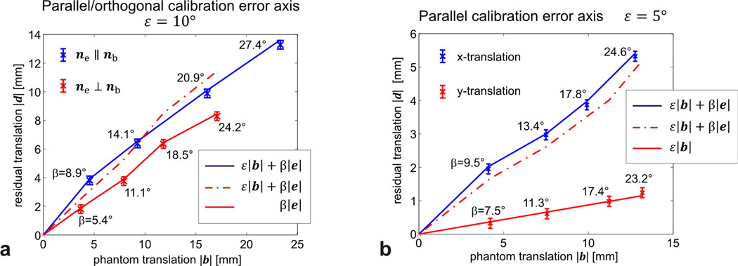
Experimental verification of the translation error components for various relative orientations of the error and motion axes. For each translation/error pair the corresponding rotation is displayed next to the data point. In a the orientation of the calibration error axis is parallel (blue) and orthogonal (red) to the phantom rotation. In b the direction of the translational error is varied between the scanner’s x- and y-axis.

Figure 3b shows results when there is a 5° calibration error parallel to the phantom rotation. Again, there is excellent agreement between the measured translations (blue crosses) and theoretical values (blue solid line) if the requirements of Lemma 2 are fulfilled (translational error in calibration co-linear to translation). In contrast, the data shown in red represent results when Lemma 2 is violated by translating the true cross-calibration along the y-axis and shifting the phantom along the x-axis. In this instance, the residual translations measured (red crosses) are substantially below the upper bound calculated from Eq.[19] (dashed dotted red line). The measured values can then be calculated accurately by omitting the second term of Eq.[19] (solid red line); specifically, n_e is parallel to n_b and e which makes e − ÊB̂Ê⁻¹e zero, so that only the rotation of b by Ê remains.

Figure 4 shows the central sagittal slice of the in vivo volumetric brain scans. Figure 4a serves as a reference since head motion, as measured by the tracking camera, is virtually zero. The image quality of Figure 4b with a perfectly calibrated external tracking system and head motion (approximately ±5°) is almost identical to the reference scan, although some artifacts are visible in the regions of the tongue and the neck where the rigid-body assumption is very likely violated. In Figure 4c (1° miscalibration), the image shows declined spatial resolution and a ringing artifact across the whole image, although head motion was comparable to that in Figure 4b.

Figure 4.

Sagittal slices of a volumetric structural scan with prospective motion correction enabled and the corresponding head motion traces. Figure 4a serves as a reference since no head motion was present. In b and c moderate head motion with comparable amplitude and frequency was detected. For perfect cross calibration the result is shown in b, and for c the calibration error was set to 1°.

Discussion

We derived simple analytical expressions for the rotational and translational components of residual motion correction errors due to imperfect cross-calibration of an external tracking device. All theoretical results were verified experimentally with the help of phantom experiments and intentional calibration errors. Within the intrinsic measurement accuracy of the sparse phantom method [11] we found perfect agreement between the theoretical predictions and the measured deviations (Figures 2 and 3). Since a Taylor approximation of the sinusoidal terms was used, the validity of our results is limited to small rotation angles. However, the theoretical predictions are in excellent agreement with the experimental results for motion and calibration error angles up to 20°. This range is rarely exceeded in a realistic situation; calibration errors are typically on the order of 1° or less, and head rotations seldom exceed 10°with typical head cushioning.

The residual rotational component shows a bi-linear dependence upon the rotational calibration error and the degree of motion performed, modulated by the sine of the angle between the calibration error and the motion axes (see Eq.[15]). Therefore, if the rotation axis of the calibration error and that of the object motion are parallel, no rotational tracking error occurs. Conversely, the residual tracking error is maximized if the two rotation axes are orthogonal. The residual translation error is bounded by the sum of the rotation angle multiplied by the translational component of the calibration error plus the calibration error angle multiplied by the length of the actual displacement (see Eq.[19]). We demonstrated that this upper bound of the residual displacement error is only reached if three conditions are met: the error and motion rotation axes are parallel, the error and motion translations are parallel, and the translation vector is orthogonal to the rotation axes.

In our analysis, the residual motion D only depends on the relative transformation between the true and the estimated camera position (Eq.[8]), whereas the cross calibration X has no influence on D. This is in contrast to the work presented by Aksoy [7], which found that the residual tracking error was dependent on the absolute camera position and, in turn, on the distance between the camera and MRI isocenter. We traced this apparent discrepancy to a difference in the definition of the error term in the cross calibration. Specifically, Aksoy et al. assumed the camera to be at a fixed position relative to MR isocenter and then introduced a rotational error with the rotation center at the actual camera position. In the scanner frame, this off-center rotation induces a secondary displacement that depends on the absolute camera position and scales with the camera-to-scanner distance. Conversely, our approach effectively separated rotational from translational errors.

While calibration errors and object movements were tightly controlled in the current study, these two measures, and their relationships, are generally unknown in a real-world situation, and object motion is pseudo-random. However, Equations [16] and [19] provide strict upper bounds for residual tracking errors, and make it possible to calculate the calibration accuracy required to achieve a certain tracking accuracy. Furthermore, if one considers subject motion random, then the resulting tracking errors will essentially be random as well. In this situation, Maclaren et al. demonstrated that the tracking noise, or random residual tracking errors in our case, has to be less than ¼ of the pixel resolution to ensure image quality is not affected [12], assuming a signal-to-artifact ratio of 100. Therefore, for a typical pixel size of 1 mm for clinical MRI, tracking errors should not exceed 0.25 mm or 0.25° (for a pixel 60 mm off isocenter). If we additionally assume head rotations up to 10° in patients, then calibration errors of less than 1° will ensure rotational tracking errors are within 0.2°. The error propagation for translations is more complex since both the rotation error and the translation error contribute to the residual translation. For example, a 1 mm/1° calibration error in combination with a 10 mm/10° head movement can result in a residual translation of 0.35 mm after the correction is applied. However, the combination of 1° calibration error with approximately 8° head rotation degraded in-vivo image quality of a volumetric MPRAGE structural scan. This is likely because a semi periodic head movement was performed, that leads to a consistent phase variation pattern in k-space, which has more dramatic effects on the reconstructed images than a randomly distributed error in k-space as was assumed in [12]. While a semi-periodic head movement is not likely to occur in real patients, this observation emphasizes the need for accurate cross-calibration in motion correction with external tracking devices.

Conclusion

We demonstrate that for moderate head rotations (<20°) the maximum residual rotational error in motion corrected scans is given by the product of the calibration error and the performed head rotation. The translation error has two contributions: The object translation weighted by the rotational calibration error component plus the object rotation multiplied with the translational calibration error component. These simple expressions for the residual tracking errors were verified experimentally and make it possible to determine the cross calibration accuracy required for a specific motion compensation accuracy. For typical applications, successful prospective motion correction using an external tracking device requires that the calibration accuracy is substantially below 1 mm and 1°.

Appendix

One way of representing a homogenous transform matrix H is given by separating the rotational and the translational component

$$\mathit{H}=(\begin{array}{cc}\widehat{\mathit{R}}& \mathit{t}\\ 0& 1\end{array})\underset{¯}{\underset{¯}{\text{def}}}(\widehat{\mathit{R}},\mathit{t})$$ [A.1]

Where R̂ is a 3×3 unitary rotation matrix and t a 3×1 translation vector.

Applying the transform to an arbitrary vector × is then given as

$$(\widehat{\mathit{R}},\mathit{t})·\mathit{x}=\widehat{\mathit{R}}\mathit{x}+\mathit{t}$$ [A.2]

Accordingly, multiplication of two homogenous transforms A and B is given as

$$(\widehat{\mathit{A}},\mathit{a})·(\widehat{\mathit{B}},\mathit{b})\equiv (\widehat{\mathit{A}},\mathit{a})·(\widehat{\mathit{B}}\mathit{x}+\mathit{b})=\widehat{\mathit{A}}(\widehat{\mathit{B}}\mathit{x}+\mathit{b})+\mathit{a}=\widehat{\mathit{A}}\widehat{\mathit{B}}\mathit{x}+\widehat{\mathit{A}}\mathit{b}+\mathit{a}\equiv (\widehat{\mathit{A}}\widehat{\mathit{B}},\widehat{\mathit{A}}\mathit{b}+\mathit{a})$$ [A.3]

It is easy to verify that the inverse of a homogenous transform is given as

$${(\widehat{\mathit{R}},\mathit{t})}^{-1}=({\widehat{\mathit{R}}}^{-1},-{\widehat{\mathit{R}}}^{-1}\mathit{t})$$ [A.4]

Any rotation matrix A can be expressed as a rotation around an axis a = (a₁,a₂,a₃) about an angle α.

$$\mathit{A}=1+{\omega }_a\text{sin}\alpha +{\omega }_a^2(1-\text{cos}\alpha ),$$ [A.5]

where ω_a is a skew-symmetric matrix populated with the components of the rotation axis a

$${\omega }_a=(\begin{array}{ccc}0& -a_3& a_2\\ a_3& 0& -a_1\\ -a_2& a_1& 0\end{array})$$ [A.6]

Multiplying ω_a with an arbitrary vector x has the same effect as the cross product a × x.

Lemma 1 (validity of Eq.17)

“For small angles β, the following approximation is valid: |e − ÊB̂Ê⁻¹e| ≤ |βe| for β ≪ 1.”

Proof: As noted, the sandwich equation ÊB̂Ê⁻¹ represents a coordinate transformation. Therefore, ÊB̂Ê⁻¹ preserves the total rotation angle β of B̂ = (β,n_b), but involves a new rotation axis denoted n_ebe, and can be represented by (β, n_ebe). The expression e − ÊB̂Ê⁻¹e represents the difference between the vector e and the vector e rotated by β about axis n_ebe. If the rotation axis n_ebe is orthogonal to e, then the rotation can be described as a 2D rotation of e with rotation angle β in the plane orthogonal to n_ebe (Figure 1b). For small rotations β ≪ 1, the length of the difference vector can be approximated by the length of an arc with radius |e| and angle, yielding |e − ÊB̂Ê⁻¹e| ≅ |βe|. The effective rotation angle will be smaller than β for any other orientation of n_ebe relative to e (non-orthogonal), and reach zero for e ∥ n_ebe. It follows that |e − ÊB̂Ê⁻¹e| ≤ |βe| for β ≪ 1 for arbitrary e, Ê, and B̂.

Lemma 2

For small rotations and in first-order approximation, the inequality |d| ≤ ε|b| + β|e| (Eq.[19]) becomes an equality when the following 3 conditions are met:

$$\mathit{b}=f\mathit{e}\text{with}f<0(\text{translation error and actual translation anti-parallel})$$ [A.7]

$$\widehat{\mathit{E}}\widehat{\mathit{B}}=\widehat{\mathit{B}}\widehat{\mathit{E}}(\text{rotation axes parallel})$$ [A.8]

$$\mathit{b}\text{and}\mathit{e}\text{are orthogonal to rotation axes of}\widehat{\mathit{E}}\text{and}\widehat{\mathit{B}}$$ [A.9]

This represents a situation where the translations involved (of the calibration error and head motion) are collinear ([A.7]), and separately the axes of rotations involved (of the calibration error and head motion) are parallel (i.e. the rotation matrices commute [A.8]).

Proof: Starting with Eq. [12], we separate the total error d into two terms:

$$\mathit{d}=\widehat{\mathit{E}}\{\mathit{b}-\widehat{\mathit{B}}{\widehat{\mathit{E}}}^{-1}{\widehat{\mathit{B}}}^{-1}\mathit{b}\}+\{\mathit{e}-\widehat{\mathit{E}}\widehat{\mathit{B}}{\widehat{\mathit{E}}}^{-1}\mathit{e}\}$$ [A.10]

Using [A.8], this simplifies to:

$$\mathit{d}=\widehat{\mathit{E}}\{\mathit{b}-{\widehat{\mathit{E}}}^{-1}\mathit{b}\}+\{\mathit{e}-\widehat{\mathit{B}}\mathit{e}\}=\{\widehat{\mathit{E}}\mathit{b}-\mathit{b}\}+\{\mathit{e}-\widehat{\mathit{B}}\mathit{e}\}$$ [A.11]

Using [A.7], we obtain:

$$\mathit{d}=\{\mathit{e}-\widehat{\mathit{B}}\mathit{e}\}-f\{\mathit{e}-\widehat{\mathit{E}}\mathit{e}\}$$ [A.12]

The first term represents the difference between the vector e and e rotated by β, and the second term represents the difference between the vector e and e rotated by ε (times factor f). Since the rotation axes of Ê and B̂ are identical and orthogonal to the vector e, it is easy to prove that for small rotations [A.12] can be approximated as :

$$\mathit{d}\approx \beta \left|\mathit{e}\right|\mathit{u}+\epsilon \left|f\mathit{e}\right|\mathit{u}=(\epsilon |\mathit{b}|+\beta |\mathit{e}|)\mathit{u}$$ [A.13]

where u is a unit vector orthogonal to both the rotation axis and the direction of e. This yields

$$\left|\mathit{d}\right|\approx \epsilon \left|\mathit{b}\right|+\beta \left|\mathit{e}\right|$$ [A.14]

and shows that inequality [19] turns into an (approximate) equality [A.14] when the conditions [A.7] through [A.9] are met. Therefore, for an unknown set of calibration errors and motion parameters, Eq. [19] provides a minimal upper bound for the tracking error |d|.

References

- 1.Aksoy M, Forman C, Straka M, Skare S, Holdsworth S, Hornegger J, Bammer R. Real-time optical motion correction for diffusion tensor imaging. Magn Reson Med. 2011 Aug;66:366–378. doi: 10.1002/mrm.22787. [DOI] [PMC free article] [PubMed] [Google Scholar]
- 2.Schulz J, Siegert T, Reimer E, Labadie C, Maclaren J, Herbst M, Zaitsev M, Turner R. An embedded optical tracking system for motion-corrected magnetic resonance imaging at 7t. MAGMA. 2012 Dec;25:443–453. doi: 10.1007/s10334-012-0320-0. [DOI] [PubMed] [Google Scholar]
- 3.Zaitsev M, Dold C, Sakas G, Hennig J, Speck O. Magnetic resonance imaging of freely moving objects: prospective real-time motion correction using an external optical motion tracking system. Neuroimage. 2006 Jul;31:1038–1050. doi: 10.1016/j.neuroimage.2006.01.039. [DOI] [PubMed] [Google Scholar]
- 4.Ehman RL, Felmlee JP. Adaptive technique for high-definition mr imaging of moving structures. Radiology. 1989 Oct;173:255–263. doi: 10.1148/radiology.173.1.2781017. [DOI] [PubMed] [Google Scholar]
- 5.Tsai R, Lenz R. A new technique for fully autonomous and efficient 3d robotics hand/eye calibration. Robotics and Automation, IEEE Transactions on. 1989;5:345–358. [Google Scholar]
- 6.Wang C. Extrinsic calibration of a vision sensor mounted on a robot. IEEE Trans. Robot. Automat. 1992;8:161–175. [Google Scholar]
- 7.Aksoy M, Ooi M, Maclaren J, Bammer R. Cross-calibration accuracy requirements for prospective motion correctionn. Proc. Intl. Soc. Mag. Reson. Med. 21, Salt Lake City. 2013 [Google Scholar]
- 8.McCarthy J. Introduction to Theoretical Kinematics. MIT press; 1990. ISBN 0262132524. [Google Scholar]
- 9.Daniilidis K. Hand-eye calibration using dual quaternions. The International Journal of Robotics Research. 1999 Mar;18:286–298. [Google Scholar]
- 10.Maclaren J, Armstrong BSR, Barrows RT, Danishad KA, et al. Measurement and correction of microscopic head motion during magnetic resonance imaging of the brain. PLoS One. 2012;7(no. 11):e48088. doi: 10.1371/journal.pone.0048088. [DOI] [PMC free article] [PubMed] [Google Scholar]
- 11.Zahneisen B, Lovell-Smith C, Herbst M, Zaitsev M, Speck O, Armstrong B, Ernst T. Fast noniterative calibration of an external motion tracking device. Magn Reson Med. 2013 Jun; doi: 10.1002/mrm.24806. [DOI] [PMC free article] [PubMed] [Google Scholar]
- 12.Maclaren J, Speck O, Stucht D, Schulze P, Hennig J, Zaitsev M. Navigator accuracy requirements for prospective motion correction. Magn Reson Med. 2010 Jan;63:162–170. doi: 10.1002/mrm.22191. [DOI] [PMC free article] [PubMed] [Google Scholar]