

Abstract
A method is presented capable of disambiguating the relative influence of statistical covariates upon neural spiking activity. The method, an extension of the generalized linear model (GLM) methodology introduced in Truccolo et al. (2005) to analyze neural spiking data, exploits projection operations motivated by a geometry present in the Fisher information of the GLM maximum likelihood parameter estimator. By exploiting these projections, neural activity can be divided into three categories. These three categories, neural activity due solely to a set of covariates of interest, neural activity due solely to a set of uninteresting, or nuisance, covariates, and neural activity that cannot be unequivocally assigned to either set of covariates, can be associated with physical variables such as time, position, head-direction and velocity. This association allows the analysis of neural activity that can, for example, be due solely to temporal influence, irrespective of other, identified, influences. The method is applied in simulation to a rat exploring a temporally modulated place field. A portion of the analysis reported in MacDonald et al. (2011), using the methodology described herein, is reproduced. This analysis demonstrates the temporal bridging of a delay period in a sequential memory task by firing activity of cells present in the rodent hippocampus that cannot be explained by rodent position, head direction or velocity.
Keywords: Neural activity disambiguation, Confound, Covariate disambiguation, Generalized linear model, Projection, Point process
1. Introduction
Understanding which biological stimuli and behavioural signals influence neural firing is a fundamental area of scientific interest in neuroscience. In many experiments, multiple, confounded signals are recorded that may influence neural spiking activity.1 While some signals may be of direct interest to experimenters, others may be ancillary to the question they are investigating, and can pose a nuisance. When both types of signals interdepend identifying signal effect upon observed spiking activity is problematic. This difficulty presents the experimenter with a number of questions. Which signals affect neural spiking? Which of these signals are of scientific interest? How should the signals that are not of direct interest be handled? To what extent can experiments be designed to remove the confounding effect of these nuisance signals? To what extent can statistical techniques handle these confounds?
Such questions arise often in neural coding studies. For example, the influence upon hippocampal neural activity by rodent position, rodent movement, odour type, and experimental condition are dissociated in Wood et al. (1999). In Wood et al. (2000) left-turn/right-turn preferential hippocampal neural activity is identified after accounting for rodent speed, heading and position. The separation of the influence of hand, joint and muscle defined coordinate systems on activity in the monkey motor cortex is addressed in Georgopoulos et al. (1986) and Wessberg et al. (2000). The separation of timing effects from spatial effects in rodent hippocampal neural activity is discussed in MacDonald et al. (2011). For pedagogical purposes, we here label one set of signals as spatial covariates and another set as temporal covariates, and discuss dissociating their influence on spiking.
There are multiple approaches used to address nuisance signal confounding. In one approach experiments are designed to eliminate the influence of confounding covariates. In another approach, data potentially affected by the confounding covariate or nuisance signal is discarded. Finally, as described in this work, the influence of nuisance signals upon neural activity can be explicitly modelled and a projection performed to effectively decouple the influence of sets of covariates upon neural spiking. This projection exploits the geometry described in Cook (1986) and McCullagh and Nelder (1999) associated with the parameter Fisher information for a large class of neural spiking models. Use of this projection yields sets of asymptotically independent model parameter estimators. The projected covariates provide information regarding the modulation of the spiking intensity due to that part of a covariate of interest that is independent of the other covariates. This unconfounded component of the neural model describes how a covariate, after accounting for the influence of the dependent and confounding covariates, affects neural spiking activity. Additionally, the parameter estimates and covariance associated with the projected signals are demonstrated to be identical to the original estimates from the confounded model. This equivalence allows assessment of the significance of the influence of any covariate on spiking, regardless of its dependence on other covariates.
A review of relevant literature and the generalized linear model statistical framework in the context of neural spike modelling is presented in Section 2. Section 3 develops statistical theory enabling the investigation of that portion of spiking influence unique to a specific covariate. Following theoretical development introduced in Section 3, the efficacy of the method is demonstrated on synthetic data produced from a temporally modulated place cell as a rat moves through the cell’s place field. The utility of the method is further demonstrated on real data analyzed in MacDonald et al. (2011). The method applied to this data, collected from a population of rodent hippocampal neurons recorded from a rat performing a sequential memory task, enables the isolation of temporally dependent neural activity that is not dependent on other covariates. The paper concludes with a discussion in Section 6.
2. Background
Geometric ideas in statistics are established and are prominent in works such as Christensen (2002), Kass (1989), Cook (1986), Cox and Reid (1986), and Lawrence (1988). The geometry in the current context, restricted to the class of generalized linear models, is first documented in Cook (1986) for the purpose of identifying leverage points, and also appears in statistical literature in the context of “orthogonal parameters”, discussed in, for example McCullagh and Nelder (1999). In neuroscience, the methodology common in fMRI analysis called Statistical Parametric Modelling (SPM) often exploits model matrices possessing some orthogonal columns, yielding orthogonal parameters within a general linear model of voxel activation. Also in the context of the general linear model, a recursive estimation algorithm is presented which exploits Gram–Schmidt orthogonalization to yield an orthogonal design matrix (Aqil et al., 2010). One notes that general linear model and generalized linear model2 are two entirely different classes of models. GLMs are appropriate for modelling data from a wide variety of distributions including Poisson counts, and history dependent point process data, and involve a non-linear “link” function relating a linear combination of covariates to the response variable. Although relevant geometric ideas are common amongst the statistics literature, the consequences of these ideas when using generalized linear models to capture covariate influence upon neuron spiking behaviour has not been discussed. This work provides a neuroscience specific treatment of the consequences of the model geometry and discusses a method for separating the influence of a set of covariates upon spiking behaviour into three parts: a first part due entirely to the covariates of interest, a second part attributed to any of the remaining covariates, and a third part with ambiguous association of the influence on spiking that cannot be attributed to these covariates. inseparable from other covariates. This latter method is used by the authors in MacDonald et al. (2011) to separate the influences of a set of temporal covariates from the influences of spatial, head directional, and speed covariates in an analysis of neural activity in rat hippocampus. We begin with a review of the generalized linear modelling (GLM) framework in Section 2.1. In Section 2.2, a review of geometric ideas central to this work is presented.
2.1. Generalized linear modelling framework
In this section, the generalized linear modelling framework (McCullagh and Nelder, 1999) and its application to spike train modelling (Truccolo et al., 2005) are reviewed. Let dnj be the jth increment of a discrete-time point-process modelling neuron spiking behaviour. Specifically, dnj is the count of the number of spikes occurring within the time interval [Δ(j – 1), Δj). For bin size Δ chosen sufficiently small, the probability, P(dnj > 1) of multiple spikes within one such interval is o(Δ). This stipulation reduces within bin history effects, limiting inaccuracy due to the time-discretization procedure. Let λj be the conditional intensity of the point process for the jth time step. The log-likelihood, , can be written
| (1) |
To construct a GLM, set the log of the conditional intensity vector, log(λ) = [log(λ1) . . . log(λN)]T, to be a linear function of a set of covariates that influence neural spiking. Specifically, let H be a design matrix with each row representing the set of covariates that influence spiking at a given time. Then the vector of the conditional intensities through time is given by
| (2) |
Here the exponentiation of a vector is defined to be element-by-element exponentiation, and β is a vector of parameters associated with the covariates.
Without loss of generality, consider the case where the design matrix H can be partitioned into two matrices, H(t) and H(s), where H(t) is used to model the influence of one set of covariates on the spiking activity, and H(s) is used to model the influence of the remaining covariates. For concreteness, refer to H(t) as the temporal covariates and H(s) as spatial covariates, although these can be any combinations of covariates whose influence one wishes to unravel. To tie the parameters with the covariates, break the model parameter vector β into β(t) and β(s). The temporal covariates are influenced by the parameters comprising β(t) and the spatial covariates are influenced by the parameters comprising β(s). Then,
The full conditional intensity vector can be expressed in terms of multiplicatively separable components related to time and space:
| (3) |
| (4) |
and
Here · is the element-by-element, or Hadamard, product between the N dimension vectors λ(s) and λ(t). While the above models are very specific, the principle described herein generalizes to arbitrary covariate sets, provided that design matrix columns are linearly independent.
The maximum likelihood estimator of β satisfies the score equations (McCullagh and Nelder, 1999). These equations result from taking the first derivative of the log-likelihood, ℓ, with respect to the parameter β, and can be written as follows:
| (6) |
where dn = [dn1 dn2 . . . dnN]T. Associated with the maximum likelihood estimate, , of the maximum likelihood estimator, , is the observed Fisher information, Ǐβ, equal to (McCullagh and Nelder, 1999)
| (7) |
Here
| (8) |
is a diagonal matrix formed from the maximum likelihood estimate of the conditional intensity, . As is shown in Section 3.2, covariate decoupling does not change the estimator of the conditional intensity. Thus, can be taken to be the standard conditional intensity estimate associated with the potentially confounded parameter estimator, . With the observed Fisher information, Ǐβ, an estimate of the Cramer-Rao lower bound,Čr, equal to
| (9) |
is available. The Cramer-Rao matrix, Cr, bounds the variance of any unbiased estimator of β. Specifically, the covariance matrix of any unbiased estimator minus the Cramer-Rao lower bound is positive semi-definite (Scharf, 1991; Casella and Berger, 2002). The maximum likelihood estimator, , attains the Cramer-Rao lower bound asymptotically (with increasing N), and thus possesses a covariance matrix, equal to Cr. Similarly, the Cramer-Rao bound estimator,Ĉr, from which the realization,Čr, specified in Eq. (9), is drawn equates to the Cramer-Rao bound in the limit when D̂ is an unbiased estimator of D. Thus asymptotically,
| (10) |
when is unbiased. In many situations of interest the parameter estimator is biased due to model mis-specification. When this occurs the conditional intensity estimator , the estimator of the diagonal matrix D̂ and the estimator of the Cramer-Rao bound,Ĉr may all be biased. In this situation, Eq. (10) is approximately correct; with an accuracy that depends on the extent of the bias. Though this bias is a concern, one notes that it is commonly thought that all models are mis-specified but that some, while mis-specified, can be used to make useful statistical inference (Box and Draper, 1987). Many model selection procedures exist and careful analysis employs their use (Truccolo et al., 2005). For the purposes of this paper, Eq. (10) is considered to be an equality. Due to the asymptotic normality of (McCullagh and Nelder, 1999), Eq. (10) completely describes the dependencies between covariate parameter estimators in the model, Eq. (2), of the neuron spiking rate, λ, as the number of measurements tends to infinity. In Section 3, based upon the dependencies specified by Eq. (10), adjustments are made to the covariates such that the un-confounded part of the covariates of interest is asymptotically independent of the remaining covariates. In the example of sets of temporal and spatial covariates, this procedure allows for a space-independent analysis of the influence of time upon a neuron's spiking behaviour.
2.2. Geometry
Let be the normed, linear vector space whose elements span . Let and be two elements of (for example, columns of H are elements of ) and define the inner-product 〈a, b〉, between a and b as
| (11) |
where D is the diagonal matrix of rates defined in Eq. (8). Then is a Hilbert space. This implies that any set of vectors can be projected with a projection operator consistent with the inner product specified by Eq. (11) onto the space formed by any other set of vectors. In the following, projections within the Hilbert space are exploited to develop a time-dependent covariate that is independent of spatial covariates and represents, heuristically, that part of time whose influence upon the neuron spike rate is unconfounded by spatial effect. In particular, the projection, P, onto the space spanned by a matrix, A, is
| (12) |
3. Covariate decoupling
In the following, two confounding groups of covariates are transformed into two new groups of covariates such that dependencies between associated parameter groups are asymptotically zero in the limit of infinite data when the conditional intensity estimate is unbiased. As discussed previously in Section 2.1, while an asymptotic result, it is found in practice to hold to good approximation with data sets of a size common to the neuroscience setting (Truccolo et al., 2005); yielding results sufficiently accurate to be useful (Cohen et al., 2007; Huang et al., 2009; Jenison et al., 2011; Saleh et al., 2010; Sarma et al., 2010; Townsend et al., 2006; Truccolo et al., 2010). This accuracy alleviates concerns regarding the convergence of the negative inverse of the observed Fisher information, Ǐβ to the covariance of the parameter estimators, , as presented in Eq. (10). For pedagogical reasons, as in Section 2.1, the two covariate groups considered in this work are the “time” group, consisting of covariates related to time, and the “space” group, consisting of covariates associated with, for example, rodent position. This designation is convenient for simplicity and fits nicely with the simulations presented in Section 4. In the data example presented in Section 5, the first group will be time and the second group is generalized to include not only covariates associated with position, but also covariates associated with speed and head direction. The language in the following is specific to two groups; but, any pairwise grouping of covariates is possible. This flexibility can be exploited to test both within covariate parameter group estimator dependency and dependencies between groups of parameter estimators.
3.1. Parameter independence
As described in Section 2.1, block diagonal implies asymptotic independence between groups of parameter estimators, and hence between the influence of groups of covariates upon neural spiking rates. Let the observed Fisher information be block diagonal,
| (13) |
where Aj is an invertible matrix for each j and 0 is a matrix of zeros of appropriate dimension. The inverse of a block diagonal matrix is a block diagonal matrix of inverted matrix blocks. That is asymptotically,
| (14) |
Thus, with the block diagonal observed Fisher information matrix, Ǐβ, specified in Eq. (13), the asymptotic maximum-likelihood parameter estimator covariance matrix, is also block diagonal.
3.2. Block diagonalization of the observed Fisher information matrix
To achieve block diagonalization of the observed Fisher information matrix, Ǐβ, specified in Eq. (7), project H(t) orthogonal to H(s) in the sense defined by the inner-product specified in Eq. (11). That is, replace the time-part, H(t) of the model matrix H with , a projection orthogonal to the range of H(s),
| (15) |
Here I is the identity matrix and is the projection matrix perpendicular to the range of H(s). The square, asymmetric projection matrix, is idempotent, possessing eigenvalues that are either zero or one and possessing the property that . Construct the modified design matrix, , which has the same range as the original model matrix H, but the component of H(t) that belongs to the span of H(s) has been removed from the time-part of the original model matrix. In words, this amounts to associating confounded neuron spiking behaviour with the spatial covariates and investigating that part of spiking behaviour which can only be explained by the effect of time. Estimation with the modified model matrix, H̃, is shown in Appendix B to yield maximum likelihood estimators, with the covariance matrix,
The observed Fisher information for is block diagonal, and thus is also block diagonal (Section 3.1). The estimators associated with the time and space covariates are asymptotically independent as described in Section 2.1. As previously discussed, this implies that functions of the time and space parameter estimators are asymptotically independent; implying that is asymptotically independent of .
3.3. Interpretation of
Fig. 1 illustrates the geometric interpretation of the projection procedure. After orthogonalization the component of each temporal covariate belonging to the span of the spatial covariates is removed.3 To maintain the pre-projection log of the conditional intensity, the parameters associated with the spatial covariates are augmented. The parameters associated with the temporal covariates are left unaffected.
Fig. 1.
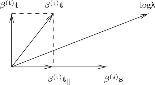
Geometry depicting the effect on model parameters due to the orthogonalization of the time covariate, t, with respect to the space covariates, here represented as a one dimensional vector, s. The superscripts, and, are withheld to emphasize the fact that this geometry applies equally to both parameter estimators and to parameter estimates. The log rate, log λ is equal to β(t)t + β(s)s. After orthogonalization, the component of t parallel to s is removed. In this situation, log λ equals β(t)t⊥ + α s, where α = β(s) + β(t)(|t∥|/|s|). Here |s| is the magnitude of the vector s. Thus, the parameter associated with time, β(t) is unaffected by the orthogonalization, while the parameter associated with space, β(s), is increased by β(t)(|t∥|/|s|).
This effect, due partly to the preservation of the range of H by the projection procedure, is demonstrated in simulation for a rat moving according to a random walk through a temporally modulated place cell (Section 4) and is depicted in Table 1 and in Fig. 4. While the time parameters are unaffected by the orthogonalization procedure, the parameters associated with the spatial covariates change to accommodate the loss of the contribution to the rate from the space-confounded part of the time covariate. This is the situation, unless the time covariate and space covariates are linearly dependent, in which case time and space are not separable. In this latter situation, there is an identifiability problem, and a unique maximum-likelihood estimator does not exist.
Table 1.
Maximum likelihood estimates for three models of neuron firing rate.
| Model type | Temporal covariate Time | Spatial covariates |
||
|---|---|---|---|---|
| Constant | Position | Squared position | ||
| Confounded | 1.31 × 10⁻³ | –10.00 | 342.44 | –5.40 × 10³ |
| Time perpendicular to space | 1.31 × 10⁻³ | –9.96 | 367.05 | –5.52 × 10³ |
| Space perpendicular to time | –6.88 × 10⁻³ | –10.00 | 342.44 | –5.40 × 10³ |
Fig. 4.

Neuron spike rates estimated using the three models. Because the range of the three different model matrices are identical, the rate estimates are also identical. This plot demonstrates this equality up to possible deviance too small to be seen on the scale plotted.
Because the parameters associated with time do not change due to projecting the time covariate perpendicular to the span of the columns of the model matrix describing the space covariates, tests of significance of temporal rate modulation un-confounded by the space covariates can be conducted using either the confounded temporal parameter estimator or by using the un-confounded temporal parameter estimator. In either case the estimators are identical and have equivalent covariance matrices. The geometry specified in Fig. 1 holds for every realization of the data, dn. That is, and are equal in realization. Thus, the covariance matrix associated with the temporal set of covariates is unchanged.
3.4. Independent rate modulation
For data sets of a size typical of neuroscience data and are independent. Due to this independence, an effect of the orthogonalization is to specify through the orthogonalized time-covariate associated with the estimator, , spiking rate behaviour that cannot be explained by the spatial covariates. As discussed in Section 3.3, tests to see if time is significant, with either the space orthogonalized or non-space-orthogonalized time covariate are identical, and the interpretation, whether or not time informs spiking behaviour, is also identical. The difference and advantage of the space-orthogonalized time-covariate becomes evident when investigating how time modulates neural spike rate. Specifically, when the time covariate is not orthogonal to the space covariate, one cannot tell whether the confounded part of the time and space covariates is associated with temporal rate modulation or with spatial rate modulation. This ambiguity is not present when the temporal covariate has been projected orthogonal to space. The identification of time-only rate modulation is used to demonstrate bridging of a delay period in a sequential memory task by a population of rodent hippocampal cells (MacDonald et al., 2011). An example analysis from MacDonald et al. (2011) is reproduced in Section 5.
3.5. Functional dependence of the projected time covariate upon spatial covariates
The orthogonalization of the time-covariate perpendicular to the space spanned by the columns of the spatial part of the model matrix introduces a positional dependence upon the time covariate. In the example of the spatial and temporal model of neural activity this dependence reflects the fact that the extent to which the effect of time on spiking rate is confounded with the effect of space on spiking rate depends on rodent movement. In particular, the orthogonalized time covariate, produced by the projection operation specified in Eq. (15), is equal to the residuals resulting from a weighted least-squares fit of the original time covariate to the spatial covariates. The weighting is equal to the estimated rate. Thus, the orthogonalized time-covariate indicates the “mis-fit” between the original non-orthogonalized time covariate and the fitted “space” model. If the rat motion is stereotyped from trial-to-trial, and further, if the position of the rat increases linearly with time, time and spatial rate effects are strongly confounded. This strong confound manifests in a span of the temporal part of the design matrix that is nearly contained within the span of the columns of the design matrix associated with space. The coordinate transformation produced by the orthogonalization procedure is demonstrated in Fig. 6. On the left of Fig. 6, the space-orthogonalized time covariate (labelled “time-perpendicular”), is plotted against the rat position for the synthetic data produced by the simulation described in Section 4. The space-orthogonalized time covariate takes on many values for any given rat position due to trial-to-trial variability in rat position, and, as described, are a scatter plot of the residuals in a weighted least-squares fit of the time covariate (across all trials) to the position related covariates. On the right-hand side of Fig. 6, the modulation of the rate due to the space-orthogonalized temporal covariate is plotted against the space-orthogonalized temporal covariate. When this covariate is zero the rate modulation is one, indicating no effect on the rate estimate due to the orthogonalized temporal covariate. This corresponds to those instances in time where the positionally dependent firing rate model suffices (with the correctly chosen parameters) to determine the time. When the original, non-projected time covariate deviates from this spatial model of time, the space-orthogonalized temporal covariate may also deviate from zero. Commensurate deviation of the rate modulation due to the space-orthogonalized temporal covariate from one indicates rate dependence on time that cannot be explained by rate influence due to the spatial covariates. In essence, firing rate modulation that can be attributed to the spatial model has been removed and any remaining modulation must arise from variation in other covariates.
Fig. 6.

Both plots: each dot corresponds to a recording instant. All 50 trials are plotted. Left: the space-orthogonalized temporal covariate vs. rat position. The functional dependence (due to orthogonal projection) of the temporal covariate upon the spatial covariates is slight. This dependence is largest at the origin where time and position are more closely linked due to the small variance of the random walk at early times. At later times, there are many values of the orthogonally projected time covariate for every rat position, due to the increased random walk variability at later times. At times approaching one, extremes in position occur and dependence between time and position seems apparent; however, in this situation few samples are available and the apparent dependence is not reliable. This plot demonstrates how the projected covariate functionally depends on the covariates it is projected orthogonal to. Because of this dependence it is not meaningful to study the temporal rate modulation using a single trial, as it would be if one were using the non-projected temporal covariate. It is necessary to summarize rate modulation over all trials with, for example, an across-trial average of the rate modulation, or a scatter plot across all trials (as shown on right) of rate modulation due to time perpendicular to space vs. time perpendicular to space. When time is explained by spatial information time perpendicular to space is zero and the rate modulation is one. Only when time perpendicular to space deviates from zero can the rate modulation due to time alone deviate from one.
3.6. Multiple covariate projections
Asymptotic independence between more than two groups of covariate parameter estimators can be obtained by performing more than one orthogonal projection. This is achieved by iteratively projecting the group of covariates that is unmodified at the time of the current projection step orthogonal to a subset of covariates within this group. For example, after projecting time orthogonal to space, one might further project some of the covariates related to space orthogonal to the remaining covariates associated with space. At the end of this procedure the observed Fisher information possesses three matrix blocks upon its diagonal. The projections can be continued in this fashion until the desired covariate separation is attained.
3.7. Inferential procedure
The proposed method of decoupling the influence of groups of covariates upon neural activity described in Section 3 augments a typical inferential procedure. Fig. 2 depicts a flow chart detailing steps in a standard-practice statistical analysis along with the methodological addition introduced in this work. This addition, represented by blue colour in the flow chart, shows the parts of an analysis affected by the methodology presented herein. The flow chart elucidates the two-part estimation procedure required to perform the covariate influence separation. In particular, one notes that the projection, Eq. (15), requires knowledge of the conditional intensity, or rate. A knowledge that is available only after preliminary parameter estimation (black coloured part of Fig. 2). Note that the rate estimate is not affected by the covariate projections. This invariance is important because if the rate estimate changed when computing rate estimates with the projected covariates the results would be inconsistent with the rate used to compute the covariate projections.
Fig. 2.

A flow chart depicting a standard statistical procedure in black with the proposed augmentation in blue. Arrows indicate sequential steps in the analysis. One notes that an estimate of the conditional intensity is required prior to forming projected covariates; an unnecessary requirement when performing linear regression. The interpretation step, also coloured blue, is part of a traditional procedure. For this step, the blue colouring indicates that the interpretation step is modified to incorporate the results of the augmented procedure. (For interpretation of the references to color in this figure legend, the reader is referred to the web version of the article.)
Model selection, described in Fig. 2, is a key part of the inferential procedure. The results presented in this paper are valid for multiplicatively separable generalized linear models using a log-link function. While this limits the class of models available at the model selection step, this class of models has produced adequate fits for data collected from many neural systems, including Truccolo et al. (2005) and MacDonald et al. (2011) and is capable of fitting a wide-range of spiking behaviour. Because of this, unless there is reason apriori to expect model mis-specification or problems with model interpretation, the multiplicatively separable generalized linear model is an excellent choice when beginning the analysis procedure. As shown schematically in Fig. 2, statistical inference is an iterative procedure whereby models are selected, analyzed and modified iteratively. Model selection procedures are detailed in Truccolo et al. (2005) and McCullagh and Nelder (1999) and are useful; both when determining model adequacy and when performing model modification.
4. Simulation
Statistical features of the proposed methodology are illustrated by simulation. Synthetic neuron spike-times are generated by a time-modulated place cell as a rat explores one spatial dimension. Data is generated for fifty trials. On each trial the rat trajectory is a realization of a random walk with drift. In Fig. 3, neural spike times, rat position, and the actual rate of neural firing are shown for the 50 simulated trials. The synthetic data is fit to three models. The first model is comprised of four covariates, the first accounting for background firing rate, the second accounting for the temporal modulation of the rate and the third and fourth accounting for spatial effects. Specifically, the model follows the form specified in Eq. (3), with the model matrix, H(t) specified to be a single column of times referenced to the beginning of each trial. Thus, this crate repeats with trial. The spatial part of the model, H(s), is specified to have three columns. The first column is constant, representing a background firing rate, the next column is the position of the rat, and the final column is the squared position of the rat. The second model is identical to the first model with the exception that the temporal covariate is replaced with its projection orthogonal to the range of H(s), employing Eq. (15). The third model is identical to the first model, with the exception that now the columns of H(s) are projected orthogonal to H(t). Maximum likelihood parameter estimates for these three models are tabulated in Table 1.
Fig. 3.

Synthetic data obtained for a time-modulated place-cell. Fifty trials obtained from a rat moving according to a random walk with drift. Raster plot (upper left), rat position vs. time (upper right), each trajectory corresponds to a single trial. Position modulation of the rate (middle left), time modulation of rate (middle right). Actual rate as a function of position and time (bottom left), and the actual rate as a function of time and trial (bottom right). The variance of the random walk insures that different parts of the place field are observed at the same time as trial varies. Note that as the variance of the random walk tends to zero, space and time become inseparably confounded. In this situation, , the design matrix, H̃ has linearly dependent columns, and the parameters associated with time and space become unidentifiable.
As described in Section 3.2, the parameter estimates for the model comprised of non-projected covariates, labelled “Confounded” in Table 1, representing a standard model for this type of analysis, yields temporal maximum likelihood parameter estimates that are identical to the maximum likelihood parameter estimates obtained with the model labelled “Time Perp. to Space”. This latter model possesses a temporal covariate projected orthogonal to the span of the columns of the design matrix associated with the spatial covariates. Similar effects consistent with the discussion in Section 3.3 are demonstrated for the other parameter estimates and models. The spike-rate estimates computed using the three models are plotted in Fig. 4. The estimates are, as expected, visually identical. In Fig. 5 estimates of the asymptotic correlation matrices of the maximum likelihood parameter estimators are shown.
Fig. 5.

Asymptotic maximum likelihood estimator correlation matrix estimates for the confounded model (left), for the time perpendicular to space model (middle), and for the space perpendicular to time model (right). The constant term is associated with the spatial covariates so that the time column in the design matrix is projected orthogonal to the constant vector as well as the position and squared position columns in the “time perpendicular to space” model. The projection successfully eliminates the approximate –20% correlation between the time and space covariates in the confounded model (far left).
These estimates are computed using Eq. (10) with the appropriate model matrices. The projections successfully remove a negative 20% correlation between the non-projected temporal covariate parameter estimator and the position covariate parameter estimator. In Fig. 6, the space-orthogonalized temporal covariate is plotted against rat position (left) and the modulation due to the space-orthogonalized temporal covariate is plotted against the space-orthogonalized temporal covariate (right). Each black dot corresponds to a recording instant. There are many values of the orthogonally projected time covariate for every position, due to trial-by-trial variability in rat position at the same within-trial temporal instant. The plot on the left-hand-side of Fig. 6 demonstrates how the projected covariate functionally depends on the covariates it is projected orthogonal to. Because of this dependence it is not meaningful to study the temporal rate modulation using a single trial, as it would be if one were using the non-projected temporal covariate. It is necessary to summarize rate modulation over all trials with, for example, an across-trial average of the rate modulation, as used on real data in Section 5, or a scatter plot across all trials, as shown on the right-hand-side of Fig. 6. As discussed in Section 3.5, modulation of the rate due to the orthogonally projected temporal covariate can deviate from one only when the weighted fit of the time covariate by the spatial covariates fails to explain the time. The importance of the temporal covariate on the rate is evident.
5. Data
The method of identifying neuron spike rate modulation specific to temporal covariates and independent of other covariates, presented in Section 3, is applied to tetrode recordings from single neuron activity in the rodent hippocampus (MacDonald et al., 2011). In this experiment, rats were trained to distinguish sequences of two events separated in time by a delay. For each sequence repetition, or trial, one of two objects is first presented. Following an empty 10-s gap, one of two odours is presented (see Fig. 1 in Kesner et al. (2005)). Electrophysiological data was collected over many trials, and on each trial, the rat, to obtain a reward, had to remember the first event in the event sequence in order to respond appropriately to the second event in the event sequence. This paradigm provides an opportunity to explore how neurons encode a sequence of events and how their activity bridges an identical temporal gap shared by distinct event sequences. One of the striking findings of this study is that individual neurons become active at different times during the delay between events and that they activate sequentially to bridge this delay (MacDonald et al., 2011). Thus, in this experimental paradigm, a natural question is to what extent, and in what fashion, is neural activity associated with the empty delay influenced by time and to what extent is it influenced by other covariates such as rat position, head direction and speed.
The portion of the analysis presented in MacDonald et al. (2011) employing the methodology presented in this work, uses a model of the log of each neuron’s spike rate, log (λ), as a seventh order polynomial model in time, a second order polynomial model of rat position, a second order polynomial of rat speed, and two head direction covariates allowing for firing rate modulation specific to a single head direction. In addition to these covariates, all second order interactions among the non-temporal covariates are included, along with the addition of two extra covariates allowing preferential velocity modulation of the firing rate. Thus the model represents place, velocity and direction “fields”, as well as temporal firing rate modulation. The total number of parameters in the model of the firing rate of each neuron is 35. The eight temporal covariates are projected orthogonal to the remaining covariates using the projection operator, Eq. (15), adjusted to include along with the space covariates discussed in conjunction with Eq. (15) in Section 3, the additional covariates relevant to this analysis; that is, speed, head direction, and interactions. As discussed in Section 3, the estimated rate modulation due to the orthogonalized time covariate is unconfounded by the non-temporal covariates. This modulation is then down-weighted by the 95% confidence interval divided by four and then averaged across trials. The down-weighting discounts highly uncertain firing rate modulation due to the orthogonally projected temporal covariates. The procedure, repeated for every neuron in four experiments yields Fig. 8 after sorting the neurons and normalizing. The de-correlation of the projected temporal covariate parameter estimators from the remaining covariate parameter estimators is demonstrated in Fig. 7. In this figure, the sum of absolute correlations between all orthogonally projected temporal covariates and the remaining covariates is computed for all neurons from all rats included in the population temporal modulation figure presented in Fig. 8, prior to the orthogonalization procedure and after the orthogonalization procedure. The resulting figures of merit, plotted in Fig. 7, demonstrate the efficacy of the procedure.
Fig. 8.

Rodent hippocampal cell activity, due to that part of temporal modulation independent of confounds, bridges a delay epoch in a sequential memory task (MacDonald et al., 2011). Each image represents the normalized, uncertainty down-weighted rate modulation due to the temporal covariates alone for a population of neurons from a different rat after averaging across trials. “Time cells” bridge the delay epoch.
Fig. 7.

The ratio of two figures of merit indicating the effect of the orthogonalization procedure on the correlation between temporal and non-temporal covariates for the data described in Section 5. The first figure of merit, indicating the extent of correlation between temporal and non-temporal covariates prior to orthogonalization, is labelled SACoriginal in the plot. The second figure of merit, identical to the first but computed using parameters estimated for a model with temporal covariates projected orthogonal to the non-temporal covariates, is labelled SACprojected in the plot. The figure of merit in both cases equals the sum of absolute correlations between temporal and non-temporal covariate parameters and is computed using the maximum likelihood parameter estimates for the relevant model. The orthogonalization procedure suppresses the sum of absolute correlation by at least approximately two orders of magnitude, and typically by six orders of magnitude. Note that the maximum value of the figure of merit is equal to the number of temporal parameters multiplied by the number of non-temporal parameters, which in this case is 216. Thus an upper bound on the correlation between a temporal covariate parameter and a non-temporal covariate parameter after temporal covariate orthogonalization is 0.02 for all but 4 neurons.
6. Discussion
A method of understanding the effect of parameter estimator dependence is provided when fitting multiplicatively separable generalized linear models of neural spiking activity. This method, described in Section 3, exploits geometry to construct independent parameter estimators associated with the original dependent parameter estimators. This procedure provides insight into the effect of pre-orthogonalization parameter estimator dependence. It is found in Section 3, due to the invariance of both parameter maximum likelihood estimates and parameter covariance matrices upon the parameter decoupling procedure, also presented in Section 3, that the identification of the significance of covariate influence upon spiking rate can be conducted ignoring dependent parameters present in the model. While this is valid, one notes that the parameter estimates are sensitive to the inclusion of confounding covariates in the model; implying that inference is valid only to the extent that the model captures salient features of the data. This is a standard caveat in statistical analysis. While tests of significant effect upon rate can be carried out without employing the orthogonalization procedure described in Section 3, the orthogonalization procedure provides a mechanism by which firing rate modulation due to a dependent covariate can be investigated independent of the effects of the remaining covariates in the model. This ability is demonstrated in simulation in Section 4 and on real data in Section 5.
In this paper, relationships between variables are modelled. The nature of this relationship is statistical in nature and is restricted to the indication of which variables can be used to explain the behaviour of which other variables. One notes that while causal relations are studied, the problem of determining which relationships are causal and which have merely a statistical, or probabilistic relation, cannot be directly solved with the methods presented.
The development within this paper, with the exception of Section 5 using real data, uses temporal and positional covariates for pedagogical reasons. While developed using only two groups of covariates, the results of this work hold for an arbitrarily large number of covariate groups. Similarly, discrete Poisson models of neuron spiking activity are used throughout this work. Generalization to the doubly-stochastic discrete-time point process setting, where the firing activity of a neuron depends upon past firing activity of the neuron, is immediate. This work provides a principled approach to the isolation of covariate effect upon neural spiking and will be of use both when analyzing data with potential confounds, but also when assessing the feasibility of investigations at the design of experiment phase.
Acknowledgements
This work was partially supported by grants from the National Science Foundation [IIS-0643995] the National Institute of Neurological Disorders and Stroke [R01 NS073118] and National Institute of Health grants MH71702 and MH096297.
Appendix A. Properties of the Matrix Projection
Some mathematical properties of the projection matrix, P, defined in Eq. (12) are specified. In particular, P, is square, asymmetric and idempotent; the eigenvalues of P are either zero or one. Additionally, let P⊥ = I – P, then,
| (16) |
| (17) |
Appendix B. Covariance Matrix Block Diagonalization
The maximum likelihood estimator, , possesses an asymptotic covariance matrix, , equal to,
Where the identities specified in Eq. (16) and in Eq. (17) have been used. Both the observed Fisher information and the asymptotic covariance of are block diagonal.
Footnotes
Here signal explicitly refers to input information available to a neuron that may, or may not, influence its spiking activity. Note that a neuron’s spiking activity in turn “signals” neurons, by relaying all or a part of the information available to it. In the following, discussion focuses upon disambiguating the effect of input neuronal signals upon neural spiking activity; however, it applies equally well to disambiguating the informational content present in the “signal” a neuron provides.
The acronym, “GLM”, is here reserved for the class of generalized linear models. This is consistent with, for example Truccolo et al. (2005) and the MATLAB™ glmfit() command.
In the following, a temporal covariate orthogonalized in this fashion is referred to as a “space-orthogonalized time covariate” or as a “space-orthogonalized temporal covariate”.
References
- Aqil M, Hong K-S, Jeong M-Y. Orthogonal functions based estimation of fnirs signal strength as GLM parameters, in the course of real-time brain activation detection.. 2010 international conference on control automation and systems (ICCAS); 2010.pp. 2244–7. [Google Scholar]
- Box GEP, Draper NR. Empirical model-building and response surfaces. Wiley; 1987. [Google Scholar]
- Casella G, Berger RL. Statistical inference. 2nd edition Duxbury Press; 2002. [Google Scholar]
- Christensen R. Plane answers to complex questions: the theory of linear models. 3rd edition Springer; 2002. [Google Scholar]
- Cohen JY, Pierre P, Woodman GF. Difficulty of visual search modulates neuronal interactions and response variability in the frontal eye field. Journal of Neural Physiology. 2007;98(5):2580–7. doi: 10.1152/jn.00522.2007. [DOI] [PubMed] [Google Scholar]
- Cook RD. Assessment of local influence. Journal of the Royal Statistical Society Series B (Methodological) 1986;8(2):133–69. [Google Scholar]
- Cox DR, Reid N. Orthogonality and approximate conditional inference. Journal of the Royal Statistical Society Series B (Methodological) 1986;49(1):1–39. [Google Scholar]
- Georgopoulos A, Schwartz A, Kettner R. Neuronal population coding of movement direction. Science. 1986;233(4771):1416–9. doi: 10.1126/science.3749885. [DOI] [PubMed] [Google Scholar]
- Huang Y, Brandon MP, Griffin AL, Hasselmo ME, Eden UT. Decoding movement trajectories through a T-Maze using point process filters applied to place field data from rat hippocampal region CA1. Neural Computation. 2009;21:3305–34. doi: 10.1162/neco.2009.10-08-893. [DOI] [PubMed] [Google Scholar]
- Jenison RL, Rangel A, Oya H, Kawasaki H, Howard MA. Value encoding in single neurons in the human amygdala during decision making. The Journal of Neuro-science. 2011;31(1):331–8. doi: 10.1523/JNEUROSCI.4461-10.2011. [DOI] [PMC free article] [PubMed] [Google Scholar]
- Kass RE. The geometry of asymptotic inference. Statistical Science. 1989;4(3):188–219. [Google Scholar]
- Kesner RP, Hunsaker MR, Gilbert PE. The role of ca1 in the acquisition of an object-trace-odor paired associate task. Behavioral Neuroscience. 2005 Jun;119(3):781–6. doi: 10.1037/0735-7044.119.3.781. [DOI] [PubMed] [Google Scholar]
- Lawrence AJ. Regression transformation diagnostics using local influence. Journal of the American Statistical Association. 1988;83:1067–72. [Google Scholar]
- MacDonald C, Lepage K, Eden U, Eichenbaum H. Hippocampal. Neuron. 2011;“time cells” bridge the gap in memory for discontiguous events.71(4) doi: 10.1016/j.neuron.2011.07.012. [DOI] [PMC free article] [PubMed] [Google Scholar]
- McCullagh P, Nelder JA. Generalized linear models. 2nd edition Chapman & Hall/CRC; 1999. [Google Scholar]
- Saleh M, Takahashi K, Amit Y, Hatsopoulos NG. Encoding of coordinated grasp trajectories in primary motor cortex. The Journal of Neuroscience. 2010;30(50):17079–90. doi: 10.1523/JNEUROSCI.2558-10.2010. [DOI] [PMC free article] [PubMed] [Google Scholar]
- Sarma S, Eden U, Cheng M, Williams Z, Hu R, Eskandar E, et al. Using point process models to compare neural spiking activity in the subthalamic nucleus of Parkinson's patients and a healthy primate. IEEE Transactions on Biomedical Engineering. 2010 Jun;57(6):1297–305. doi: 10.1109/TBME.2009.2039213. [DOI] [PMC free article] [PubMed] [Google Scholar]
- Scharf LL. Statistical Signal processing: detection, estimation, and time series analysis. Addison-Wesley Publishing Company Inc; 1991. [Google Scholar]
- Townsend BR, Paninski L, Lemon RN. Linear encoding of muscle activity in primary motor cortex and cerebellum. Journal of Neurophysiology. 2006;96(5):2578–92. doi: 10.1152/jn.01086.2005. [DOI] [PubMed] [Google Scholar]
- Truccolo W, Eden UT, Fellows MR, Donoghue JP, Brown EN. A point process framework for relating neural spiking activity to spiking history neural ensemble and extrinsic covariate effects. Journal of Neurophysiology. 2005 Feb;93(2):1074–89. doi: 10.1152/jn.00697.2004. [DOI] [PubMed] [Google Scholar]
- Truccolo W, Hochberg LR, Donoghue JP. Collective dynamics in human and monkey sensorimotor cortex: predicting single neuron spikes. Nature Neuroscience. 2010 Jan;13(1):1163–78. doi: 10.1038/nn.2455. [DOI] [PMC free article] [PubMed] [Google Scholar]
- Wessberg J, Stambaugh CR, Kralik JD, Beck PD, Laubach M, Chapin JK, Kim J, Biggs SJ, Srinivasan MA, Nicolelis MAL. Real-time prediction of hand trajectory by ensembles of cortical neurons. Nature. 2000;408(6810):1416–9. doi: 10.1038/35042582. [DOI] [PubMed] [Google Scholar]
- Wood ER, Dudchenko P, Robitsek RJ, Eichenbaum H. Hippocampal neurons encode information about different types of memory episodes occurring in the same location. Neuron. 2000;27(3):623–33. doi: 10.1016/s0896-6273(00)00071-4. [DOI] [PubMed] [Google Scholar]
- Wood ER, Dudchenko PA, Eichenbaum H. The global record of memory in hippocampal neuronal activity. Nature. 1999;397(6720) doi: 10.1038/17605. [DOI] [PubMed] [Google Scholar]