Inferring Group-wise Consistent Multimodal Brain Networks via Multi-view Spectral Clustering

Abstract

Quantitative modeling and analysis of structural and functional brain networks based on diffusion tensor imaging (DTI) and functional MRI (fMRI) data have received extensive interest recently. However, the regularity of these structural and functional brain networks across multiple neuroimaging modalities and also across different individuals is largely unknown. This paper presents a novel approach to inferring group-wise consistent brain sub-networks from multimodal DTI/resting-state fMRI datasets via multi-view spectral clustering of cortical networks, which were constructed upon our recently developed and validated large-scale cortical landmarks - DICCCOL (Dense Individualized and Common Connectivity-based Cortical Landmarks). We applied the algorithms on DTI data of 100 healthy young females and 50 healthy young males, obtained consistent multimodal brain networks within and across multiple groups, and further examined the functional roles of these networks. Our experimental results demonstrated that the derived brain networks have substantially improved inter-modality and inter-subject consistency.

I. Introduction

Studying structural/functional brain networks via diffusion tensor imaging (DTI)/functional magnetic resonance imaging (fMRI) has attracted increasing interest recently due to their potential in elucidating fundamental architectures and principles of the brain [1], [2]. Taking brain regions as nodes and the structural connections or functional correlations between these regions as edges, the brain can be viewed as a graph, and thus can be analyzed using graph theory principles in computer science [3]. For instance, a variety of recent analysis on brain networks via graphical approaches have shown that both functional and structural networks of human brain share multiple properties with common complex networks (e.g., social network), including small-worldness, scale free (a few highly-connected hubs) and modularity [1], [4–10]. Furthermore, it is reported that the structural network modularity plays a key role in generating persistent and dynamic functional patterns [11] and also determining the hierarchical functional architectures [12], [13]. Thus, constructing brain networks that are structurally and functionally meaningful and consistent is crucial to unveiling the brains' fundamental principles [14], [15].

Among tremendous efforts in exploration of brain networks, many of them adopt the single MRI imaging technique, although their approaches may be different. For instance, some studies used information from MRI to obtain brain modules. In [16], six structural modules in brain that have the firm correspondences with brain functional regions were revealed by comparing brain cortical thickness measured by MRI. In addition, more studies used the advanced diffusion imaging technique such as diffusion tensor imaging (DTI) and diffusion spectrum imaging (DSI) to construct brain structural networks and obtain corresponding structural clusters. In [8], an analysis on large-scale brain structural networks constructed by DSI reveals a structural core in the posterior medial and parietal cerebral cortex, together with several modules. On the other hand, thanks to the powerful technique of fMRI, in vivo analysis of human brain functional network becomes possible. For instance, in [17], the resting state module of human brain has been analyzed by comparing fMRI BOLD signals under task with the ones in resting state (R-fMRI).

Essentially, these studies might be substantially improved by integrating multimodal information [2]. It has been shown that anatomical structural network connections play a key role in determining and maintaining functional patterns [1]. In general, better quantitative characterization of the relationship between multimodal brain networks and its consistency across individuals could significantly advance our understanding of the human brain architectures. However, this important issue has been rarely investigated due to the following challenges. First, the variability across individuals makes it difficult to define reliable regions of interest (ROIs) that has group-wise consistency. In general, most brain parcellation approaches have difficulty in establishing across-subjects correspondences. This problem has been overcome by warping brains into an atlas space via image registration algorithms and further use the manually-segmented regions in the atlas as ROIs despite of its limitations in accuracy and robustness [18]. Another set of methods from the functional perspective is using task-based fMRI to detect functionally-corresponding ROIs [17]. Nevertheless, the cost and time in fMRI data acquisition, is the major restriction in obtaining data for large-scale networks and for large populations. Thus, it is very challenging to acquire large-scale group-wise consistent ROIs upon which to construct brain networks. Second, it is also very challenging to achieve the consistency between structural and functional brain networks that are derived from different imaging modality, i.e., DTI and R-fMRI, respectively. As shown in Fig. 1, and also as reported by Honey et al.[19], there is significant variability between functional and structural networks which makes it difficult to define and detect common networks between modalities.

Fig. 1.

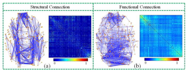
An example of the constructed structural (a) and functional (b) brain networks. Both networks were composed upon the same set of 358 DICCCOL ROIs as nodes. Each sub-figure shows a joint view of ROIs (orange dots) and their connections (blue lines), along with the corresponding connectivity matrix on the right.

In response to the abovementioned challenges, this paper presents a novel approach to infer group-wise consistent brain networks from multimodal DTI/R-fMRI datasets via multi-view spectral clustering of large-scale cortical landmarks and their connectivity graphs. Specifically, we defined network nodes by our recently developed and validated brain landmarks, namely DICCCOL (Dense Individualized and Common Connectivity-based Cortical Landmarks) [20]. As shown in Fig. 1, the DICCCOL system at the current stage is composed of 358 cortical landmarks, each of which was optimized to possess consistent group-wise DTI-derived fiber connection patterns across populations [20], [21]. The neuroscience basis is that each cortical region's cytoarchitectonic area has an unique set of extrinsic inputs/outputs (called the “connectional fingerprint” [22]), which generally predicts the function that each cortical area could possibly possess. According to our extensive structural and functional validations [20], these landmarks possess structural and functional consistency and preserve correspondences across individuals. Based on these landmarks, we constructed both structural and functional brain networks using multimodal DTI/R-fMRI data for 150 healthy young adult brains (aged 17-28 years old, with 100 females and 50 males) [23]. We equally separated these subjects into three groups (2 groups of females and 1 group of male) for the purpose of comparison and reproducibility examination. Then, we developed and applied an effective multi-view spectral clustering algorithm to derive the consistent multimodal brain networks. Specifically, we considered each structural or functional network in a subject as a separate view of the studied large-scale network, and then modeled the clustering of group-wise consistent multimodal brain sub-networks in an unified multi-view clustering framework, by which the substantial variability of large-scale brain networks across modalities (DTI and R-fMRI) and different individuals (50 subjects in each training group) can be modeled and handled by the powerful multi-view spectral clustering method. The prominent advantage of multi-view spectral clustering methodology is that it can effectively deal with heterogeneous features by maximizing the mutual agreement across multimodal clusters in different views [24]. This is actually the major methodological novelty and contribution of this paper.

II. Method

In this section, we will introduce our computational pipeline of the proposed algorithm, which is summarized in Fig. 2. First, after obtaining 358 whole-cortex dense landmarks based on our recently developed DICCCOL [20], we constructed the functional connections and structural connections between these DICCCOL landmarks with the R-fMRI and the DTI, which will be detailed in section II.A. Based on this, we trained each pair of connectivity matrices, subject by subject, to obtain the common connections across modalities while retaining individual information of each subject, and then trained and combined these pair-wise common matrices group-wisely. The respective co-training algorithms will be introduced in section II.C. In the end, the final group-wise multi-modality common connectomes are obtained using spectral clustering, as will be described in section II.B.

Fig. 2.

Illustration of the computational pipeline of the proposed method.

A. Multimodal Brain Network Construction

In response to the first challenge, i.e., to acquire large-scale group-wise consistent ROIs upon which to construct brain networks, we recently developed and validated 358 cortical landmarks that have intrinsically-established structural and functional correspondences in different brains [20], which provides the natural and ideal nodes for brain network construction. Based on these 358 cortical landmarks/ROIs (Fig. 1), we constructed both structural (Fig. 1a) and functional (Fig. 1b) networks for 150 healthy brains with multimodal DTI/R-fMRI data. Specifically, to construct structural connection matrix, the connection strength between each pair of ROIs is defined as the average FA (fractional anisotropy) value along the fiber bundle connecting these two ROIs. If there is no connecting fiber bundle between two ROIs, the connection strength is set to 0. As for the connectivity matrix of functional networks, they are constructed based on R-fMRI data as follows. First, we performed brain tissue segmentation directly on DTI data [25], and used the gray matter segmentation map as a constraint for R-fMRI BOLD signal extraction. A principal component analysis was then conducted for the R-fMRI time series of all gray matter voxels within an ROI, and the first principal component was adopted as its representative R-fMRI BOLD signal. Finally, the functional connection strength between ROIs is defined as the Pearson correlation of their R-fMRI BOLD signals. An example of the constructed structural and functional networks is shown in Fig. 1.

B. Spectral Clustering

Taking a graph G=(V,E) with ‖V‖=n nodes, the objective of clustering problem is to find cluster indicator matrix C=ℜ^n×k such that for the i^th column of C, c_ij = 1 iff. the j^th node belongs to the i^th cluster. Otherwise, c_ij = 0. The spectral clustering algorithm solves this problem by solving the following equation [26]:

$$(D-W)y=\lambda Dy$$ (1)

where W = ℜ^n×n is the affinity/similarity matrix of G, which is a semi-positive definite matrix. D is a diagonal matrix with the degree $d_i={\sum }_{j=1}^n{w}_{ij}$ for the corresponding vertex v_i on its diagonal. Meanwhile, Eq. 1 can be formulated as eigen problem of Laplacian matrix L = I−D⁻¹W [27]. When the eigenvalue of L equals to 0, the corresponding eigenvector y is the cluster indicator vector c of the graph. For the non-zero eigenvalue of L, the first k eigenvectors of L, corresponding to the k smallest eigenvalues, is the approximation of C that partitions the graph into k components. The objective of this solution is to partition the graph by the normalized cut (Ncut) [27], which is defined as:

$$\mathit{\text{Ncut}}(A,B)=\frac{\mathit{\text{cut}}(A,B)}{\mathit{\text{assoc}}(A,V)}+\frac{\mathit{\text{cut}}(A,B)}{\mathit{\text{assoc}}(B,V)}$$ (2)

where A∪B = V, and A∩B = Φ. cut(A,B) = Σ_u∈A,v∈Bw_uv is the sum of edges connecting partitions A and B, which is called cut in graph theory. assoc(A,V) = Σ_i∈Ad_i is the total connections from nodes in A, and assoc(B,V) is defined in a similar way. By minimizing Ncut value, one tends to obtain a balanced partition with relatively low cut.

In practice, the second eigenvector of graph Laplacian is often used to bi-partition the graph. As shown in Fig. 3, we can partition the nodes by their signs in the second eigenvector – that is, assigning the nodes with the positive value in the eigenvector to one cluster and the rest to the other. However, to achieve more meaningful result, k-means algorithm is applied to bi-partition the graph based on the second eigenvector. Then, the sub-graph can be further partitioned by recalculating the eigenvector of the graph Laplacian of sub-graph if necessary. By doing so recursively, the graph will be partitioned into multiple clusters. Specifically, we applied Ncut as determinant condition for bi-partitioning. We will stop bi-partitioning sub-graph if Ncut value is larger than the pre-set threshold. Thus, the number of clusters will be determined by the threshold we set. The outline of this partition algorithm is listed below, by following [26].

Fig. 3.

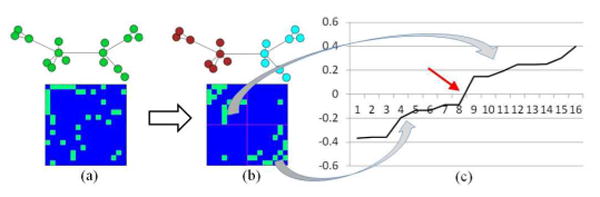
Illustration of spectral clustering. (a) The original graph and the corresponding affinity matrix. (b) The clustered graph and the corresponding affinity matrix re-arranged by clusters. (c) The second eigenvector of the graph after sorting.

Algorithm 1. Spectral Clustering
Input: Connectivity matrix W with size n×n, and the threshold T of Ncut for partitioning.
Output: Clusters of nodes.
1.	Compute the normalized Laplacian L of W.
2.	Solve eigenvectors of L with the smallest eigenvalues.
3.	Use the eigenvector with the second smallest eigenvalue to bi-partition the graph, and then compute the corresponding Ncut value.
4.	If Ncut < T, bi-partition the graph, and repeat the algorithm on two bi-partitioned sub-graphs.
5.	Else Return without bi-partitioning the graph.

C. Co-Training Approach Based on Spectral Clustering

In our research problem, we have both structural connectivity and functional connectivity for large-scale brain network clustering. To find common brain sub-networks across different modalities, an intuitive way is to assign a weight to each view or modality and then combine them together. However, it is difficult to define optimal weights, especially when there exists significant variability across modalities – the common connection obtained may be biased when the connection is strong in one modality but absent in the other modality. Thus, how to fuse these multimodal networks to achieve the relatively consistent sub-networks becomes an important issue. Recently, a clustering methodology called multi-view clustering has been developed to solve this type of problem [24], [28]. In this paper, we designed a co-training approach based on spectral clustering to maximize, first, the agreement between the structural network and functional network, and then the agreement between subjects, to find the group-wise consistent multimodal connectomes of the human brain.

As shown in the previous section, when the eigenvalue is 0, the corresponding eigenvector of normalized Laplacian of a graph is the cluster indicator vector. For a fully-connected graph, spectral clustering solved a relaxed solution of min cut problem. That is, the top eigenvectors carry the most discriminative information for graph clustering. In [24], the authors have shown that, by projecting the affinity matrix to the eigenspace of the first k eigenvectors corresponding to the k smallest eigenvalues, the inter-cluster details will be discarded and only the essential information required for clustering retains. Thus, we can achieve the agreement between two views by projecting the affinity matrix of one view to the eigenspace of the other view. As the eigenvectors are orthogonal, the affinity matrix in eigenspace can be easily projected back by multiplying the transpose of eigenvectors matrix. It should be mentioned that the post-projected affinity matrix obtained in this way is not symmetric. To make it symmetric, we added the post-projected affinity matrix with its transpose and then divide it by 2. The whole projection process can be summarized as follows:

$$\mathit{\text{proj}}(W,U)=(U{U}^{T}W+{(U{U}^{T}W)}^T)/2$$ (3)

where U = ℜ^n×k is the first k eigenvectors corresponding to the top k smallest eigenvalues of graph Laplacian of affinity matrix.

To further illustrate how this approach works, we assume that there exist two discriminate clusters A and B in a graph G, and also that the affinity matrix of G has been rearranged by clusters as follows:

$$W=\left[\begin{array}{cc}{W}_A& W_{AB}\\ W_{AB}^T& W_B\end{array}\right]$$ (4)

where W_A = (ℜ)^{‖A‖×‖A‖} are the edges between nodes in cluster A, with W_B defined similarly. W_AB = ℜ^{‖A‖×‖B‖} are the edges between clusters A and B. Then the corresponding cluster indicator matrix C is:

$$C=\left[\begin{array}{cc}{I}_A& 0\\ 0& I_B\end{array}\right]$$ (5)

where I_A = 1^‖A‖, I_B = 1^‖B‖. As W_A and W_B are the symmetric matrices, let's define $E_A=I_A{I}_A^T=1^{\Vert A\Vert \times \Vert A\Vert }$ and $E_B=I_B{I}_B^T=1^{\Vert B\Vert \times \Vert B\Vert }$. Then, we can get:

$$\begin{array}{l}{W}^{\ast }=\mathit{\text{proj}}(W,C)\hfill \\ =(C{C}^{T}W+{(C{C}^{T}W)}^T)/2\hfill \\ =\frac{1}{2}\left[\begin{array}{cc}{E}_A{W}_A& E_A{W}_{AB}\\ E_B{W}_{AB}^T& E_B{W}_B\end{array}\right]+\frac{1}{2}{\left[\begin{array}{cc}{E}_A{W}_A& E_A{W}_{AB}\\ E_B{W}_{AB}^T& E_B{W}_B\end{array}\right]}^T\hfill \\ =\frac{1}{2}\left[\begin{array}{cc}{E}_A{W}_A+W_A{E}_A& E_A{W}_{AB}+W_{AB}{E}_B\\ E_B{W}_{AB}^T+W_{AB}^T{E}_A& E_B{W}_B+W_B{E}_B\end{array}\right]\hfill \\ =\left[\begin{array}{cc}{W}_A^{\ast }& W_{AB}^{\ast }\\ {W_{AB}^{\ast }}^T& W_B^{\ast }\end{array}\right]\hfill \end{array}$$ (6)

We can see that the element w_ij of $W_A^{\ast }$ is the average degree of entry i and entry j of sub-matrix W_A, which are similarly done for $W_B^{\ast }$ and $W_{AB}^{\ast }$. This indicates that the projection process tends to fuse and smooth the inter-cluster connections or intra-cluster connections independently. As we know, the intra-cluster connections tend to be high and inter-cluster connections are relatively low. By smoothing inter/intra-cluster connections separately, we can expect the increase in intra-cluster connection strength and vice versa. However, in practice, the eigenvectors obtained are approximations of cluster indicators, and the clusters are indicated by their signs approximately as shown in Fig. 3. Then, for the above affinity matrix W, the corresponding second eigenvector should be:

$$U=\left[\begin{array}{c}P\\ N\end{array}\right]$$ (7)

where P = ℜ^‖A‖ is containing the positive real numbers and N = ℜ^‖B‖ is a vector containing the negative real numbers. Then we will have:

$$\begin{array}{ll}{W}^{\ast }\hfill & =\mathit{\text{proj}}(W,U)\hfill \\ \hfill & =(U{U}^{T}W+{(U{U}^{T}W)}^T)/2\hfill \\ \hfill & =\frac{1}{2}\left[\begin{array}{cc}P{P}^T{W}_A+P{N}^T{W}_{AB}^T& P{P}^T{W}_{AB}+P{N}^T{W}_B\\ N{N}^T{W}_{AB}^T+N{P}^T{W}_A& N{N}^T{W}_B+N{P}^T{W}_{AB}\end{array}\right]+\frac{1}{2}{\left[\begin{array}{cc}P{P}^T{W}_A+P{N}^T{W}_{AB}^T& P{P}^T{W}_{AB}+P{N}^T{W}_B\\ N{N}^T{W}_{AB}^T+N{P}^T{W}_A& N{N}^T{W}_B+N{P}^T{W}_{AB}\end{array}\right]}^T\hfill \\ \hfill & =\frac{1}{2}\left[\begin{array}{cc}P{P}^T{W}_A+W_A^{T}P{P}^T& P{P}^T{W}_{AB}+W_{AB}N{N}^T\\ N{N}^T{W}_{AB}^T+W_{AB}^{T}P{P}^T& N{N}^T{W}_B+W_B^{T}N{N}^T\end{array}\right]+\frac{1}{2}\left[\begin{array}{cc}P{N}^T{W}_{AB}^T+W_{AB}N{P}^T& P{N}^T{W}_B+W_A^{T}P{N}^T\\ N{P}^T{W}_A+W_B^{T}N{P}^T& N{P}^T{W}_{AB}+W_{AB}^{T}P{N}^T\end{array}\right]\hfill \\ \hfill & =\left[\begin{array}{cc}{W}_A^{\ast }& W_{AB}^{\ast }\\ {W_{AB}^{\ast }}^T& W_B^{\ast }\end{array}\right]\hfill \end{array}$$ (8)

In the above equation, $W_A^{\ast }$ can be separated into two parts. The first part $(P{P}^T{W}_A+W_A^{T}P{P}^T)/2$ is the fuse of connections within cluster A, and the second part $(P{N}^T{W}_{AB}^T+W_{AB}N{P}^T)/2$ is the fuse of connections between clusters A and B. It should be noted that the first part is all positive and the second part is all negative, which means $W_A^{\ast }$ is the sum of intra-cluster connections of cluster A minus the inter-cluster connections between A and B. Similarly, $W_B^{\ast }$ is the sum of connections in B minus the inter-cluster connections. And $W_{AB}^{\ast }$ is the sum of inter-cluster connections minus the intra-cluster connections. As we know, W_A and W_B are the matrices that are relatively dense with large values, and W_AB is sparser with low values. Thus, we can expect high positive values evenly distributed in $W_A^{\ast }$ and, $W_B^{\ast }$ while low or even negative values in $W_{AB}^{\ast }$. Since the negative values in W^∗ are caused by strong inter-cluster connections which are the disagreed part between the matrices and are in conflict with the definition of the affinity matrix, we set all negative values in W^∗ to 0 after projection.

Let $U=\left[\begin{array}{cccc}{u}_1& u_2& \dots & u_k\end{array}\right]={\Re }^{n\times k}$ be the combination of the first k eigenvectors, and then we will have:

$$\mathit{\text{proj}}(W,U)=\sum _{i=1}^k\mathit{\text{proj}}(W,u_i)$$ (9)

Thus, by projecting the graph affinity matrix to the eigenspace of top eigenvectors of corresponding graph Laplacian matrix, we can smooth and thus increase the intra-cluster connections and also decrease or remove inter-cluster connections. Let $M=\text{∑}_{i=1}^k{u}_i{u}_i^T$ be the projecting matrix. For pair-wise co-training of functional and structural connectivity matrices, we can project functional matrix to the spectral eigenspace of structural matrix and vise versa at the same time by using above steps iteratively. While for group-wise co-training process, we can project the matrices of one subject to the spectral eigenspace of the rest subjects. The group-wise co-training step for p subjects with single view for each subject is defined as follows:

$$\mathit{\text{gproj}}(W_i,U_{\mathit{\text{all}}})=((\sum _{j=1,j\ne i}^p{M}_j)W_i+({(\sum _{j=1,j\ne i}^p{M}_j)W_i)}^T)/2$$ (10)

where W_i is the affinity matrix of subject i; U_j is the spectral eigenvector matrix of subject j; $M_j=U_j{U}_j^T$ is the corresponding projecting matrix of subject j. When we have both structural matrix and functional matrix for each subject, M_j is re-defined as $U_{Sj}{U}_{Sj}^T+U_{Fj}{U}_{Fj}^T$, where U_sj is the eigenvector matrix of structural matrix spectrum, and U_Fj is the eigenvector matrix of functional matrix spectrum. W_i is then either the functional matrix or structural matrix. The detailed algorithm for pair-wise co-training is as Algorithm 2.

As shown previously, during the projection process, the within-cluster connection will be smoothed (increasing the positive agreement between matrices) and the disagreed connections will be broken (increasing the negative agreement between matrices). As a result, only the agreed connections will be retained during the iterative projection. As the algorithm will converge when no more agreement could be further achieved, the convergence could be assessed by the measurement of similarity between matrices. Particularly, we applied different measurements for different scenarios and will discuss this important issue in details in section I.A.

Algorithm 2
Input: Connectivity matrices of two views $W_1^0$, $W_2^0$ , and the number of eigenvectors to consider k.
Output: Co-trained connectivity matrices $W_1^{\ast }$, $W_2^{\ast }$.
1.	Compute the initial normalized Laplacian $L_1^0$ , $L_2^0$of each connectivity matrix, and the first k eigenvectors $U_1^0$ , $U_2^0$ with the k smallest eigenvalues of $L_1^0$ , $L_2^0$.
2.	for i = 1 to iter
3.	$W_1^i=\mathit{\text{proj}}(W_1^{i-1},U_2^{i-1})$
4.	$W_2^i=\mathit{\text{proj}}(W_2^{i-1},U_1^{i-1})$
5.	Compute Laplacian and the corresponding first k eigenvectors $U_1^i$ , $U_2^i$ of $W_1^i$ , $W_2^i$.
6.	If converge, return $W_1^{\ast }=W_1^i,W_2^{\ast }=W_2^i$.

The algorithm for group-wise co-training algorithm is similar to the above by replacing the pair-wise projection function proj() to the group-wise projection function gproj() in Eq. 10. After co-training, the trained matrices are similar as shown in section IV.A. The final fused connection matrix can be obtained by calculating the average normalized matrix between different subjects and views. Base on fused connection matrix, the final multi-modal connectomes of human brain will be obtained directly by applying spectral clustering algorithm in section II.B.

III. Experiment Material and Parameter Selection

A. Experiment Materials

Our experiment was performed on 150 healthy adults (100 females and 50 males) from the publicly released dataset by the Beijing Normal University, China [23]. Both DTI and R-fMRI were acquired for each subject. The parameters are as follows. R-fMRI: 33 axial slices, thickness/gap = 3/0.6mm, in-plane resolution = 64×64, TR = 2000ms, TE = 30ms, flip angle = 90°, FOV = 200×200mm. DTI: single-shot Echo-Planer Imaging-based sequence, 49 axial slices, 2.5mm slice thickness, TR = 7200ms, TE = 104ms, 64 diffusion directions, b-value = 1000s/mm², matrix = 128×128, FOV = 230×230mm². Preprocessing steps include tissue segmentation, surface reconstruction, and fiber tracking, which are similar to the methods in [20]. Then a set of large-scale, group-wise consistent ROIs were obtained for each subject using the method in [20]. The structural and functional connectome matrices were then computed using the method described in section II.A. Examples of ROIs and connectivity matrices are shown in Fig. 1. To test the reproducibility of our proposed method, we randomly separated the female subjects into two training groups: female group 1 and female group 2.

B. Parameter Selection

Normalized mutual information (NMI) [29] and Pearson correlation coefficient (PCC) are applied as measurements to assess the level of agreement between two affinity matrices. NMI between two affinity matrices A and B is defined as follows:

$$\mathit{\text{NMI}}(A,B)=\frac{I(A,B)}{[H(A)+H(B)]/2}$$ (11)

where $H(A)=-\text{∑}_{i,j}P(a_{ij})logP(a_{ij})$ is the entropy of A. I(A,B) is the mutual information between A and B, and is defined as:

$$I(A,B)=\sum _{i,j}\sum _{p,q}P(a_{ij},b_{pq})log\frac{P(a_{ij},b_{pq})}{P(a_{ij})P(b_{pq})}$$ (12)

The values of NMI and PCC are both between 0 and 1. The higher the value is, the more the two matrices agree with each other [29].

Number of eigenvectors

During the co-training process introduced in section II.C, the affinity matrix will be projected to the first k eigenvectors of the graph Laplacian. In ideal case, k should be set equal to or larger than the true cluster number. However, due to the lack of prior knowledge, we tested the result with different k values on the pair-wise training of single subject networks. As shown in Fig. 4(a)-(b), by using small k value, more information will be removed and thus the agreement between two views will be higher. However, small k value will cause the loss of useful information and results in over-training. Also, small k value may cause oscillation during training process which is vulnerable. On the other hand, large k value will keep too much information including the uncommon information between views that we want to remove and thus may cause under-training. Considering that the number of nodes in our network is 358, we set k to 25 empirically. By using this k value, we can ensure the useful information retained, and also the accuracy and smoothness during training process.

Fig. 4.

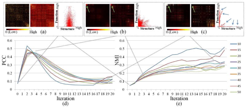
Illustration of parameter selection for pair-wise training. (a)-(c) Original structural and functional connections and the co-trained connections in the 3^rd and 18^th iteration when the top 25 eigenvectors are considered. In each subfigure, the left figure is structural matrix; the middle figure is functional matrix; the right figure is functional connection vs. structural connection with each dot representing an edge. (d) Changes of PCC during co-training iteration with different numbers of eigenvectors considered. (e) Changes of NMI during co-training iteration with different numbers of eigenvectors considered.

Convergence criterion

During the training process, our goal is to maximize the agreement between different views. In Fig. 4(e), we can see that the NMI between two networks is increasing during the training process. In general, PCC between two networks increases in the first several iterations rapidly and then decreases slowly. This is mainly because there is a certain amount of disagreement between two networks. Though the intra-cluster connections will be smoothed to increase the agreement between two matrices, some connections may still be relatively weak compared with other connections as highlighted by green arrows in Fig. 4(b)-(c). Also, as highlighted by the blue arrows in Fig. 4(c), we can see that, after training, certain sets of edges are highly correlated, but there may exist multiple correlation models between two views and thus the overall correlation is low. This indicates that, compared with PCC, NMI is a better measurement as the criterion of co-training convergence. However, the pair-wise trained result will be used for successive group-wise training. If the training process iterates for too many times, the group-wise information will also be smoothed out at the same time, although we maximize the agreement between two matrices of each subject. Thus, we use PCC value as a convergence criterion for pair-wise training (Fig. 2(b)). The mean NMI between each pair of subjects of each view is used as a convergence criterion of group-wise training (Fig. 2(c)). As shown in Fig. 5 and Supplemental Fig. 1, it takes about 30 iterations for group-wise co-training algorithm to converge. For pair-wise training, it takes either 3 or 4 iterations to converge (see Supplemental Table I).

Fig. 5.

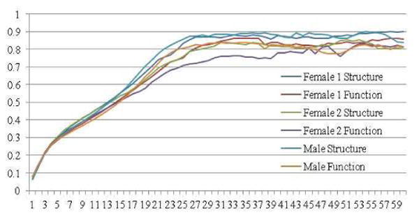
Changes of average NMI in each iteration of group-wise co-training process for each training group.

IV. Results

A. Clustered Multi-modal Networks

We obtained 8 multi-modal clusters upon 358 DICCCOL landmarks using the proposed methods and the parameters described above. The clustering results are similar when set threshold of Ncut in spectral clustering algorithm from 0.2 to 0.9, thus we set it 0.5 specifically. We randomly picked 4 subjects in female group 1 and visualized their affinity matrices before and after training in Fig. 6, where the matrices are all rearranged by clusters. Each cluster is highlighted by a green box. As the connection strength of edges in certain cluster may be relatively higher which makes it difficult to visualize other clusters (Fig. 4 (d-e)), the connection strength of co-trained matrices are adaptively normalized for the purpose of visualization in the following way. First, each row of matrix is scaled independently such that the largest element in each row is 1 (i.e., by normalizing the largest connection to each node). Then, add the row-normalized matrix to its transpose to obtain the adjusted matrix (symmetrizing matrix). By observation, we can see that the connection matrices vary substantially between subjects and modalities before optimizations (the second row of each panel). After pair-wise co-training, the structural connection matrix and functional connection matrix of each subject are more similar to each other, but there still exists disagreement. However, after group-wise training, the matrices are similar across subjects and modalities. A clear boundary of eight clusters can be observed (at the third row of each panel). To validate the performance of the proposed algorithm in identifying common clusters, the strengths of the original structural/functional connections within each cluster are measured as shown in Table I. Obviously, both of the average structural connection and the average functional connection within each cluster are substantially higher than the average connection strength of the whole brain network. Similar observation can also be observed in the first rows of the matrices in Fig. 6 that the clusters inferred by the proposed algorithm have relatively stronger within-cluster connections than the whole network for both connection matrices.

Fig. 6.

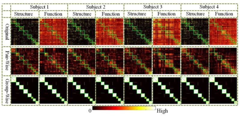
Visualization of original and trained connection matrices of 4 randomly selected subjects from the first female group. The matrices are re-arranged by group-wise consistent clusters. Each cluster is highlighted by green box. The matrices are adaptively normalized node by node to give better visualization.

Table I. Average Connection Strengths.

	Whole Brain	Cluster 1	Cluster 2	Cluster 3	Cluster 4	Cluster 5	Cluster 6	Cluster 7	Cluster 8
Structure	0.037	0.118	0.104	0.098	0.062	0.070	0.090	0.092	0.193
Function	0.249	0.284	0.353	0.264	0.348	0.301	0.263	0.334	0.329

We visualized the 8 clusters trained from the female group 1 on the cerebral cortex surface in Fig. 7(a)-(c). By observation, most of the clusters are composed by ROIs that are geometrically close to each other or structurally/functionally connected. It is interesting that the parcellation of the cortical landmarks in Fig. 7(a)-(c) largely coincides with the recently published clusters obtained via genetic similarity by Chen et al. [32] and is consistent with current neuroscience knowledge. For instance, the major part of cluster 1 includes the visual cortex [7], [33–36]. The major part of cluster 4 includes the sensory-motor systems including pre- and post-central gyrus (BAs 1/2/3/4), and the Supplementary Motor Area (SMA) (BA 6) [7], [34–36]. Cluster 8 includes the prefrontal cortex (BA 11) and dorsal anterior cingulate (BA 32) [34]. Fig. 7(d) shows the average structural connections between clusters. More intra-cluster connections than inter-cluster connections can be observed. We can also observe connection hubs within each cluster such as DICCCOL #104, #170, #185, #200 in cluster 4 as highlighted by black arrow. For details of location of these DICCCOL ROIs on the cerebral cortex, please refer to the website (http://dicccol.cs.uga.edu).

Fig. 7.

Visualization of group-wise multimodal brain networks computed based on the female training group 1. The color-coding of sub-networks is provided in the right side of subfigure (d). (a)-(c) Visualization of multi-modal sub-networks on template cerebral cortex. The visualization was generated by ParaView [30]. (d) Visualization of average structural connections between ROIs. Only the top 9.17% connections (the average connection density of 150 structural matrices applied) are retained. ROIs are rearranged and color-coded by sub-networks and listed around the circle. Between sub-networks connections are represented by gray lines and within sub-network connections are represented by corresponding color lines. The visualization was generated using the Circos toolkit [31]. It should be noted that the short distances of the re-arranged connections in this sub-figure do not necessarily mean that their actual structural connections have short distances, as shown in (a).

B. Reproducibility and Between-Gender Similarity

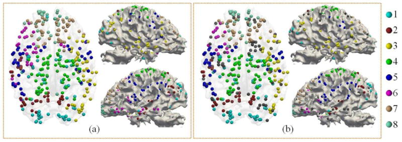
The female training group 2 also generated 8 clusters. The visualization of these 8 clusters on the template cortex surface is shown in Fig. 8(a). The IDs of clusters are calibrated according to their overlap degree with the clusters of female group 1. The nodes with consistent cluster labels between two female training groups are shown in Fig. 8(b). By observation, we can clearly see that these eight clusters are similar to those obtained from female group 1. Besides, we further computed the Rand Index (RI) [37] and NMI [29] between clustering results of these two sets of subjects. Both RI and NMI range between 0 and 1. The higher value indicates higher similarity between clustering results. As shown in Table II, the RI value between these two results is 0.93 and the NMI value is 0.72. These relatively high RI and NMI values suggest that the proposed method is stable and robust, and the results are highly reproducible across different training groups.

Fig. 8.

Visualization of group-wise multimodal brain networks computed based on female training group 2. The visualization is performed on the template brain with Paraview [30]. Corresponding sub-networks are color-coded by the same color. (a) Networks of female training group 2. (b) Nodes with consistent clusters between two female training groups. Inconsistent nodes are color-coded by gray.

Table II. RI and NMI Between Clustering Results.

Index Type	RI	NMI
Female 1 VS. Female 2	0.93	0.72
Female 1 VS. Male	0.94	0.77
Female 2 VS. Male	0.93	0.74

The training results on male groups also gave eight similar clusters. As shown in Fig. 9, it is evident that the male's multi-modal clusters are similar to those of females. The RI and NMI values between the clustering results of male and female groups are also high (Table II). There are 298 nodes that are consistent in cluster labels between two female training groups and 282 consistent nodes across all three training groups. As previous neuroscience studies suggested that there is a certain degree of difference in brain function and structure between genders [38], it is intriguing that no significant difference can be observed between the obtained network clusters of male and female. Our interpretation is that the DICCCOLs we applied as ROIs do not carry much gender-specific information [20]. To further quantitatively show this point, we measured the NMI between the original connection matrices and no significant differences between genders can be observed (Supplemental Fig. III). As for the network disagreement between females and males, it is still not clear whether they are caused by sexual difference, or by the variability in the data acquisition, preprocessing and analysis. However, as shown in Fig. 8(b) and Fig. 9(b), the most inconsistent nodes locate on the boundary region between clusters. It is more likely that the variability between cluster results is caused by the individual variability. This observation, together with previous results, suggests that the proposed multi-view spectral clustering algorithm is robust and powerful in identifying group-wise consistent clusters.

Fig. 9.

Visualization of group-wise multimodal brain networks computed based on male training group. The visualization is performed on the template brain with ParaView [30]. Corresponding sub-networks are color-coded by the same color. (a) Networks of male training group. (b) Nodes with consistent clusters across three training groups. Inconsistent nodes are color-coded by gray.

C. Comparisons between Approaches

For the purpose of comparison, sub-networks obtained by different approaches are computed. We computed the group-wise sub-networks based only on structural information or only on functional information. The group-wise consistent connection matrix for each modality is obtained respectively using the proposed multi-view spectral co-training approach. The parameters are selected in a way similar to those described in section III.B. As there is only one connection matrix considered for each subject, group-wise co-training is performed directly on the original matrices without pare-wise co-training. On average, it took 42 iterations for structural matrices to converge and 36 iterations for functional matrices to converge. The threshold of Ncut in the spectral clustering is set to 0.5. Also, an average matrix of both modalities' connection matrices of the training group is obtained for comparison. Based on the average matrix, the cluster is obtained by the spectral clustering method described in section II.B. As the matrix is more densely connected compared with the final fuse matrices obtained by proposed approach, the threshold of Ncut is set to 0.9 here. In this section, our analysis will mainly focus on the results of female group 1. For the results of other training groups, it is referred to supplemental Fig. 2-3.

In total, 14 structural clusters and 11 functional clusters were obtained. These clusters can be visually observed with clear boundaries in Fig. 10(b)-(c). The visualization of clusters on the template cortex is shown in Fig. 11. Interestingly, functional regions are symmetric in certain degree between the left and right spheres. Another intriguing observation is that, though structure connection matrix generated more clusters, these clusters are highly reproducible across three training groups we have. As shown in Table III, the average RI value is 0.97 and average NMI value is 0.83, which are relatively high.

Fig. 10.

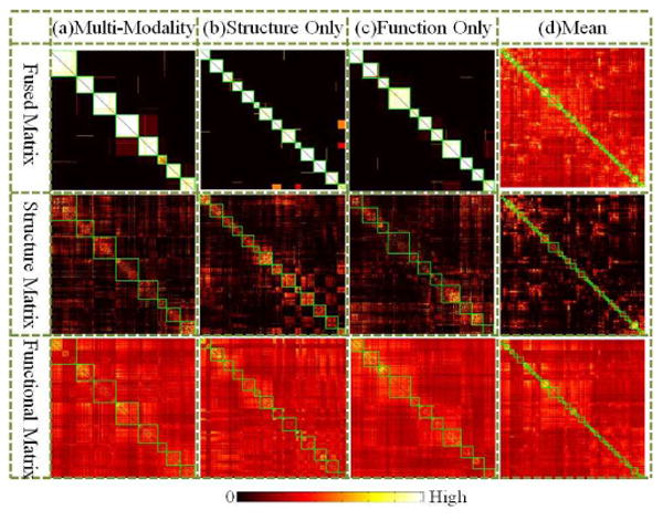
Visualization of clusters on matrices obtained by different approaches from female group 1. Matrices including adaptively normalized fused matrix (top row), average structure matrix (middle row), and average functional matrix (bottom row) are visualized and rearranged by corresponding clusters. Each cluster is highlighted by green box. In each sub-figure, the IDs of the clusters from top-left to bottom-right are from 1 to n successively. (a) Fused matrix using the proposed group-wise multi-view co-training approach using multi-modality matrices. (b) Group-wise co-trained matrix fused by the proposed method with structure connection matrices only. (c) Group-wise co-trained matrix fused by the proposed method with functional connection matrices only. (d) Average matrix of both connection matrices of all the subjects in the training group.

Fig. 11.

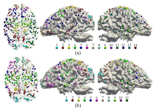
Visualization of group-wise structural/functional brain networks computed based on female group 1. The visualization is performed on the template brain with ParaView [30]. (a) Structural networks. (b) Functional networks.

Table III. RI and NMI Between Clustering Results.

	Structure		Function
Index Type	RI	NMI	RI	NMI
Female 1 VS. Female 2	0.97	0.84	0.93	0.73
Female 1 VS. Male	0.97	0.83	0.92	0.69
Female 2 VS. Male	0.96	0.82	0.92	0.70

It is evident that the derived brain sub-networks via the multi-view spectral clustering method have substantially improved inter-modality consistency in comparison with the clustering results by any single modality. As shown in Fig. 10, the clusters based only on structural connection matrices failed to give functional meaningful clusters. On the other side, functional clusters also failed to generate significant structural clusters. During the multi-modal co-training process, these single modality clusters are split and then recombined considering the mutual clusters between modalities. Thus, as shown in Fig. 10(a), the multi-modal clusters carry dense intra-cluster connections for both structural and functional connections.

However, as shown in Fig. 10(d), the average matrix failed to offer meaningful information for clusters, which might be caused by the following reasons. 1) The variability across individual connection matrices might be relatively high. Thus, by averaging individual matrices, useful information might be smoothed out. 2) The structural connection matrix is too sparse compared with functional connection matrix. Thus, the structural information may be overwhelmed by functional information. 3) The disagreement between two modalities is relatively high. For the edges between certain nodes, only the connection in one modality is strong. But the connection strength of these edges will still remain strong if taking the average value as the common connection strength.

V. Discussion and Conclusion

We inferred eight group-wise consistent multi-modal brain sub-networks via a novel multi-view spectral clustering approach based on our recently developed cortical landmark system - DICCCOL. The DICCCOL system is composed of 358 cortical landmarks, which are optimized and predicted via brain white matter connection patterns such that they possess correspondence between individuals. Structural/functional networks are composed of connections between these landmarks derived from DTI/R-fMRI data. Then a co-training framework based on the novel multi-view spectral clustering algorithm is applied to obtain the group-wise consistent and cross-modality common brain network clusters. The advantage of multi-view spectral clustering methodology is that it can effectively deal with heterogeneous features by maximizing the mutual agreement across clusters in different views [24].

Our experiment results have shown that the algorithm converges well on the data used. Eight multi-modal brain sub-networks that are reproducible across different training groups have been identified. They are also shared by both males and females. Compared with clusters derived from structural connection or functional connection only, the sub-networks obtained by our proposed method have improved inter-modality consistency significantly.

To conclude, the major technical contribution of this work is the proposed novel clustering framework for multi-view brain networks. Based on this framework, eight sub-networks are derived from the DICCCOL system via connection matrices based on DTI/R-fMRI data. Our experimental results suggest that the derived sub-networks are functionally/structurally meaningful. Also, we demonstrated the possible usage of DICCCOL system in studying brain networks patterns. Further and intensive studies based on the DICCCOL system and those eight inferred multi-modal sub-networks can potentially help elucidate brain functions and dysfunctions in the future.

References

- 1.Bullmore E, Sporns O. Complex brain networks: graph theoretical analysis of structural and functional systems. Nature reviews Neuroscience. 2009 Mar;10(no. 3):186–98. doi: 10.1038/nrn2575. [DOI] [PubMed] [Google Scholar]
- 2.Bassett DS, Bullmore ET. Human brain networks in health and disease. Current opinion in neurology. 2009 Aug;22(no. 4):340–7. doi: 10.1097/WCO.0b013e32832d93dd. [DOI] [PMC free article] [PubMed] [Google Scholar]
- 3.Watts DJ, Strogatz SH. Collective dynamics of ‘small-world’ networks. Nature. 1998 Jun;393(no. 6684):440–2. doi: 10.1038/30918. [DOI] [PubMed] [Google Scholar]
- 4.Achard S, Salvador R, Whitcher B, Suckling J, Bullmore E. A Resilient, Low-Frequency, Small-World Human Brain Functional Network with Highly Connected Association Cortical Hubs. Journal of neurosicience. 2006;26(no. 1):63–72. doi: 10.1523/JNEUROSCI.3874-05.2006. [DOI] [PMC free article] [PubMed] [Google Scholar]
- 5.Sporns O, Zwi JD. The small world of the cerebral cortex. Neuroinformatics. 2004 Jan;2(no. 2):145–62. doi: 10.1385/NI:2:2:145. [DOI] [PubMed] [Google Scholar]
- 6.He Y, Chen ZJ, Evans AC. Small-world anatomical networks in the human brain revealed by cortical thickness from MRI. Cerebral cortex. 2007 Oct;17(no. 10):2407–19. doi: 10.1093/cercor/bhl149. [DOI] [PubMed] [Google Scholar]
- 7.Salvador R, Suckling J, Coleman MR, Pickard JD, Menon D, Bullmore E. Neurophysiological architecture of functional magnetic resonance images of human brain. Cerebral cortex. 2005 Sep;15(no. 9):1332–42. doi: 10.1093/cercor/bhi016. [DOI] [PubMed] [Google Scholar]
- 8.Hagmann P, Cammoun L, Gigandet X, Meuli R, Honey CJ, Wedeen VJ, Sporns O. Mapping the structural core of human cerebral cortex. PLoS biology. 2008 Jul;6(no. 7):e159. doi: 10.1371/journal.pbio.0060159. [DOI] [PMC free article] [PubMed] [Google Scholar]
- 9.Iturria-Medina Y, Canales-Rodríguez EJ, Melie-García L, Valdés-Hernández PA, Martínez-Montes E, Alemán-Gómez Y, Sánchez-Bornot JM. Characterizing brain anatomical connections using diffusion weighted MRI and graph theory. NeuroImage. 2007 Jul;36(no. 3):645–60. doi: 10.1016/j.neuroimage.2007.02.012. [DOI] [PubMed] [Google Scholar]
- 10.Iturria-Medina Y, Sotero RC, Canales-Rodríguez EJ, Alemán-Gómez Y, Melie-García L. Studying the human brain anatomical network via diffusion-weighted MRI and Graph Theory. NeuroImage. 2008 Apr;40(no. 3):1064–76. doi: 10.1016/j.neuroimage.2007.10.060. [DOI] [PubMed] [Google Scholar]
- 11.Kaiser M, Görner M, Hilgetag CC. Criticality of spreading dynamics in hierarchical cluster networks without inhibition. New Journal of Physics. 2007 May;9(no. 5):110–110. [Google Scholar]
- 12.Müller-Linow M, Hilgetag CC, Hütt MT. Organization of excitable dynamics in hierarchical biological networks. PLoS computational biology. 2008 Jan;4(no. 9):e1000190. doi: 10.1371/journal.pcbi.1000190. [DOI] [PMC free article] [PubMed] [Google Scholar]
- 13.Zhou C, Zemanová L, Zamora G, Hilgetag C, Kurths J. Hierarchical Organization Unveiled by Functional Connectivity in Complex Brain Networks. Physical Review Letters. 2006 Dec;97(no. 23) doi: 10.1103/PhysRevLett.97.238103. [DOI] [PubMed] [Google Scholar]
- 14.Zhang T, Guo L, Li K, Jing C, Yin Y, Zhu D, Cui G, Li L, Liu T. Predicting functional cortical ROIs via DTI-derived fiber shape models. Cerebral cortex. 2012 Apr;22(no. 4):854–64. doi: 10.1093/cercor/bhr152. [DOI] [PMC free article] [PubMed] [Google Scholar]
- 15.Supekar K, Musen M, Menon V. Development of large-scale functional brain networks in children. PLoS biology. 2009 Jul;7(no. 7):e1000157. doi: 10.1371/journal.pbio.1000157. [DOI] [PMC free article] [PubMed] [Google Scholar]
- 16.Chen ZJ, He Y, Rosa-Neto P, Germann J, Evans AC. Revealing modular architecture of human brain structural networks by using cortical thickness from MRI. Cerebral cortex. 2008 Oct;18(no. 10):2374–81. doi: 10.1093/cercor/bhn003. [DOI] [PMC free article] [PubMed] [Google Scholar]
- 17.Greicius MD, Krasnow B, Reiss AL, Menon V. Functional connectivity in the resting brain: a network analysis of the default mode hypothesis. Proceedings of the National Academy of Sciences of the United States of America. 2003 Jan;100(no. 1):253–8. doi: 10.1073/pnas.0135058100. [DOI] [PMC free article] [PubMed] [Google Scholar]
- 18.Hellier P, Barillot C, Corouge I, Gibaud B, Le Goualher G, Collins DL, Evans A, Malandain G, Ayache N, Christensen GE, Johnson HJ. Retrospective evaluation of intersubject brain registration. IEEE transactions on medical imaging. 2003 Sep;22(no. 9):1120–30. doi: 10.1109/TMI.2003.816961. [DOI] [PubMed] [Google Scholar]
- 19.Honey CJ, Sporns O, Cammoun L, Gigandet X, Thiran JP, Meuli R, Hagmann P. Predicting human resting-state functional connectivity from structural connectivity. Proceedings of the National Academy of Sciences of the United States of America. 2009 Feb;106(no. 6):2035–40. doi: 10.1073/pnas.0811168106. [DOI] [PMC free article] [PubMed] [Google Scholar]
- 20.Zhu D, Li K, Guo L, Jiang X, Zhang T, Zhang D, Chen H, Deng F, Faraco C, Jin C, Wee CY, Yuan Y, Lv P, Yin Y, Hu X, Duan L, Hu X, Han J, Wang L, Shen D, Miller LS, Li L, Liu T. DICCCOL: Dense Individualized and Common Connectivity-Based Cortical Landmarks. Cerebral Cortex. 2012 Apr; doi: 10.1093/cercor/bhs072. in press. [DOI] [PMC free article] [PubMed] [Google Scholar]
- 21.Zhu D, Li K, Faraco CC, Deng F, Zhang D, Guo L, Miller LS, Liu T. Optimization of functional brain ROIs via maximization of consistency of structural connectivity profiles. NeuroImage. 2012 Jan;59(no. 2):1382–93. doi: 10.1016/j.neuroimage.2011.08.037. [DOI] [PMC free article] [PubMed] [Google Scholar]
- 22.Passingham RE, Stephan KE, Kötter R. The anatomical basis of functional localization in the cortex. Nature reviews Neuroscience. 2002 Aug;3(no. 8):606–16. doi: 10.1038/nrn893. [DOI] [PubMed] [Google Scholar]
- 23.Yan C, Gong G, Wang J, Wang D, Liu D, Zhu C, Chen ZJ, Evans A, Zang Y, He Y. Sex- and brain size-related small-world structural cortical networks in young adults: a DTI tractography study. Cerebral cortex. 2011 Feb;21(no. 2):449–58. doi: 10.1093/cercor/bhq111. [DOI] [PubMed] [Google Scholar]
- 24.Kumar A, D H., III A Co-training Approach for Multi-view Spectral Clustering. ICML. 2011 [Google Scholar]
- 25.Liu T, Li H, Wong K, Tarokh A, Guo L, Wong STC. Brain tissue segmentation based on DTI data. NeuroImage. 2007 Oct;38(no. 1):114–23. doi: 10.1016/j.neuroimage.2007.07.002. [DOI] [PMC free article] [PubMed] [Google Scholar]
- 26.Shi J, Malik J. Normalized cuts and image segmentation. IEEE Transactions on Pattern Analysis and Machine Intelligence. 2000;22(no. 8):888–905. [Google Scholar]
- 27.Luxburg U. A tutorial on spectral clustering. Statistics and Computing. 2007 Aug;17(no. 4):395–416. [Google Scholar]
- 28.Cai X, Nie F, Huang H, Kamangar F. Heterogeneous image feature integration via multi-modal spectral clustering. CVPR. 2011:1977–1984. [Google Scholar]
- 29.Witten IH, Frank E. Data Mining: Practical Machine Learning Tools and Techniques. Morgan Kaufmann; 2005. p. 560. [Google Scholar]
- 30.Henderson A. The ParaView guide: A Parallel visualization application. 2007 [Google Scholar]
- 31.Krzywinski M, Schein J, Birol İ. Circos: an information aesthetic for comparative genomics. Genome research. 2009;19(no. 9):1639–1645. doi: 10.1101/gr.092759.109. [DOI] [PMC free article] [PubMed] [Google Scholar]
- 32.Chen CH, Gutierrez ED, Thompson W, Panizzon MS, Jernigan TL, Eyler LT, Fennema-Notestine C, Jak AJ, Neale MC, Franz CE, Lyons MJ, Grant MD, Fischl B, Seidman LJ, Tsuang MT, Kremen WS, Dale AM. Hierarchical genetic organization of human cortical surface area. Science. 2012 Mar;335(no. 6076):1634–6. doi: 10.1126/science.1215330. [DOI] [PMC free article] [PubMed] [Google Scholar]
- 33.Sorg C, Riedl V, Mühlau M, Calhoun VD, Eichele T, Läer L, Drzezga A, Förstl H, Kurz A, Zimmer C, Wohlschläger AM. Selective changes of resting-state networks in individuals at risk for Alzheimer's disease. Proceedings of the National Academy of Sciences of the United States of America. 2007 Nov;104(no. 47):18760–5. doi: 10.1073/pnas.0708803104. [DOI] [PMC free article] [PubMed] [Google Scholar]
- 34.Damoiseaux JS, Rombouts SARB, Barkhof F, Scheltens P, Stam CJ, Smith SM, Beckmann CF. Consistent resting-state networks across healthy subjects. Proceedings of the National Academy of Sciences of the United States of America. 2006 Sep;103(no. 37):13848–53. doi: 10.1073/pnas.0601417103. [DOI] [PMC free article] [PubMed] [Google Scholar]
- 35.De Luca M, Beckmann CF, De Stefano N, Matthews PM, Smith SM. fMRI resting state networks define distinct modes of long-distance interactions in the human brain. NeuroImage. 2006 Feb;29(no. 4):1359–67. doi: 10.1016/j.neuroimage.2005.08.035. [DOI] [PubMed] [Google Scholar]
- 36.van den Heuvel M, Mandl R, Hulshoff Pol H. Normalized cut group clustering of resting-state FMRI data. PloS one. 2008 Jan;3(no. 4):e2001. doi: 10.1371/journal.pone.0002001. [DOI] [PMC free article] [PubMed] [Google Scholar]
- 37.Rand WM. Objective Criteria for the Evaluation of Clustering Methods. Journal of the American Statistical Association. 1971 Dec;66(no. 336):846–850. [Google Scholar]
- 38.Cahill L. Why sex matters for neuroscience. Nature reviews Neuroscience. 2006 Jun;7(no. 6):477–84. doi: 10.1038/nrn1909. [DOI] [PubMed] [Google Scholar]