Flying Drosophila stabilize their vision-based velocity controller by sensing wind with their antennae

Significance

Insects are widely appreciated for their aerial agility, but the organization of their control system is not well understood. In particular, it is not known how they rapidly integrate information from different sensory systems—such as their eyes and antennae—to regulate flight speed. Although vision may provide an estimate of the true groundspeed in the presence of wind, delays inherent in visual processing compromise the performance of the flight speed regulator and make the animal unstable. Mechanoreceptors on the antennae of flies cannot measure groundspeed directly, but can detect changes in airspeed more quickly. By integrating information from both senses, flies achieve stable regulation of flight speed that is robust to perturbations such as gusts of wind.

Abstract

Flies and other insects use vision to regulate their groundspeed in flight, enabling them to fly in varying wind conditions. Compared with mechanosensory modalities, however, vision requires a long processing delay (~100 ms) that might introduce instability if operated at high gain. Flies also sense air motion with their antennae, but how this is used in flight control is unknown. We manipulated the antennal function of fruit flies by ablating their aristae, forcing them to rely on vision alone to regulate groundspeed. Arista-ablated flies in flight exhibited significantly greater groundspeed variability than intact flies. We then subjected them to a series of controlled impulsive wind gusts delivered by an air piston and experimentally manipulated antennae and visual feedback. The results show that an antenna-mediated response alters wing motion to cause flies to accelerate in the same direction as the gust. This response opposes flying into a headwind, but flies regularly fly upwind. To resolve this discrepancy, we obtained a dynamic model of the fly’s velocity regulator by fitting parameters of candidate models to our experimental data. The model suggests that the groundspeed variability of arista-ablated flies is the result of unstable feedback oscillations caused by the delay and high gain of visual feedback. The antenna response drives active damping with a shorter delay (~20 ms) to stabilize this regulator, in exchange for increasing the effect of rapid wind disturbances. This provides insight into flies’ multimodal sensory feedback architecture and constitutes a previously unknown role for the antennae.

Animals rely on input from multiple sensory modalities to regulate their motor actions. For example, to quickly grasp an object, a human uses both vision and tactile sensing. The visual system can estimate how close the object is, but only touch can accurately determine when contact is made (1). Similarly, flying insects rely on multiple senses, including vision and mechanosensation to control their flight (2). This multimodal feedback enables them to perform aerial feats, such as chasing conspecifics (3) and rapid self-righting after takeoff (4). Our neurobiological and biomechanical understanding of these behaviors is incomplete, but physiological studies and physics-based models have helped reveal salient features (5–9).

The flight paths of flies often are structured into bouts of straight segments of forward motion, punctuated by rapid changes in heading termed body saccades (3, 10–12). During the straight segments, flies tend to maintain constant groundspeed despite changes in wind speed, suggesting the presence of an active feedback regulator (13, 14). Recent results provide some insight into the properties of this vision-based forward velocity controller, such as its dependence on the spatial and temporal frequency of the visual stimulus, and the magnitude of the underlying sensory-motor delay (15, 16). Experiments with tethered animals show that flies use mechanosensors on the antennae to regulate wing motion in response to changes in airspeed (17–21). Incident wind causes deflection of the arista, the fourth antennal segment, which vibrates at the frequency of the nearby flapping wings (19). Movement is detected by the Johnston organ (JO) and a large campaniform sensillum between the second and third antennal segments (18). There is evidence for both phasic and tonic neurons within the JO that respond to wind (22). However, little is known about how these neuron-mediated motor responses affect flight control, or how they are integrated with visually mediated responses. Work in other insects, such as hawk moths, indicates that the antennae may be used in a variety of flight control responses that complement vision, including reactions to body rotation, responses that in flies are thought to be mediated by the halteres (23, 24). Further, recent results using tethered honey bees suggest that together the antennae and visual system mediate an abdomen-up streamlining behavior that may minimize steady-state flight costs (25). Although the antennae may mediate similar behaviors in flies, in this study we focus on responses that help regulate forward flight speed.

The sensorimotor delay of the visual response that controls flight speed is roughly 50–100 ms in fruit flies (16), corresponding to 10–20 wing strokes. Such delays are expected in visual-motor reactions because of the time required for phototransduction and subsequent motion computation. When used in a feedback loop with high gain, sensor delay may lead to instability, which can manifest as a sinusoidal oscillation that grows with time for unstable systems or decays slowly for a nearly unstable system (26). In this paper, we investigated whether the time delay of the visual system has implications for the flies’ flight velocity controller. To do so, we captured flight trajectories of flies subject to impulsive gusts of wind in an automated wind tunnel. We compared the behavior of intact flies with that of flies whose airspeed response was abolished by removing the arista of the antennae. Our results indicate that arista-ablated flies showed greater groundspeed variability than intact flies, oscillating in a manner indicating a nearly unstable feedback regulator. A dynamic model derived from our data suggests that the velocity instability of arista-ablated flies arises from the long visual feedback delay, and that anantenna-mediated wind response acts as a damper to sense and abolish this instability.

Methods

Flies.

We used 2- to 3-d-old female flies, Drosophila melanogaster Meigen, descended from 200 wild-caught female specimens. As necessary, we anesthetized flies by cooling them to 2 °C. For ablation experiments, the aristae were clipped off at their base with sharpened forceps. Flies were kept on a 16:8-h light:dark cycle. Experiments started 5–9 h before the end of their subjective day and continued for 24 h. In each trial run, we placed 10–12 flies in the enclosed wind tunnel. To increase exploratory behavior, we starved the flies (while providing water) for 4–8 h before each experiment. We recorded roughly 100 trajectories per day for control flies and roughly 50 per day for arista-ablated flies. The mass of the flies averaged 1.2 mg at the start of trials. After the 24-h trial period, flies we recovered from the flight arena using a vacuum had an average mass of 1.0 mg. For modeling and analysis, we used the estimated average fly mass, 1.1 mg, for m.

Real-Time Fly Tracking Arena.

All experiments were performed in a 150 cm × 30 cm × 30 cm wind tunnel (27, 28) equipped with a visual projection system (Fig. 1A). The arena was backlit by near-infrared light-emitting diodes, and the cameras were fitted with infrared pass filters. To record the 3D position of flies in free flight, we used a custom-built real-time fly tracker (for details, see ref. 29). The tracker consisted of five Basler A602f digital video cameras capturing images at 100 frames per second and an array of computers performing image analysis to locate moving flies in each 2D view. These 2D coordinates were transmitted over a network to a central computer that triangulated the flies’ 3D positions in space. Median latency during tracking was ∼40 ms. The tracking software recorded trajectories and performed data association using an extended Kalman filter. In parallel, the software also estimated positions at each time step using a least-squares estimate based on ray projections from each camera. We used this noisier, unfiltered format for our analysis because it provided the highest time resolution for the high-speed dynamics in this study and is not subject to the specifics of the dynamic models associated with a Kalman filter.

Fig. 1.

Experiments in a free-flight fly tracking arena indicate that flies deprived of their antenna-mediated airspeed response show significantly greater groundspeed variability than intact flies. (A) We recorded flight trajectories by triangulating position using infrared cameras (29). Wide-field visual motion was generated by back-projecting a moving grating pattern onto the walls of the flight arena through a system of mirrors. (B) We generated wind gust stimuli either by using an impulsive air piston (Upper) or by opening shutters to allow air driven by a fan to pass through (Lower). (C) Overhead view of the path of flies relative to the gust apparatus and visual stimulus. (D) A random selection of 50 trajectories recorded in conditions of no wind stimulus suggests that groundspeeds of arista-ablated flies are more variable (Center) than those of intact flies (Left). This difference is significant (Levene’s test, P < 0.0001), as shown in a normalized histogram of instantaneous groundspeeds of all trajectories collected (Right).

Wind Gusts.

A voltage pulse from the tracking computer triggered the gust mechanism the moment the position estimate of a fly passed the predefined trigger plane. We used two different devices to generate gusts within the flight arena (Fig. 1 B and C). The first was a set of shutters actuated by a high-speed brushless linear motor (model P01-23 × 160; LinMot) that could open suddenly to allow the air pulled by a wind tunnel fan to flow through the flight arena. This provided a stimulus that ramped from a pregust steady state of −0.15 m⋅s⁻¹ to −0.35 m⋅s⁻¹ over a period of about 200 ms. Because the wind tunnel was designed for unidirectional flow, the fan system could produce wind velocity v_w of one polarity only. The second gust device was an air piston spanning the cross-section of the wind tunnel that was actuated by the same linear motor. The piston could move in either direction very quickly, moving 15 mm in as little as 40 ms, limited only by the motor’s force capability. When the air piston was in use, the fan of the wind tunnel was switched off. The software of the servomotor controller could be programmed to generate only one trajectory at a time, so a given population of flies in the tunnel arena was subjected to only one type of gust for each 24-h trial period.

The time courses of the gusts were measured with a hotwire anemometer at 1 kHz (MiniCTA with p55 probe; Dantec Dynamics) that was calibrated with an ultrasonic anemometer (UA6; Airflow Developments Ltd.). Gusts were identical to within 0.02 m⋅s⁻¹ at various positions across the width, height, and length of the wind tunnel arena up to within 2 cm of the walls, and were identical before and after each experimental session. The thickness of the boundary layer under conditions of steady flow was measured to be less than 2 cm, but any flight trajectories passing within that distance from the walls were eliminated from further analysis. To verify that there was no spatial dependence in the timing of the gust in the arena, two hotwire probes were placed 1 m apart at either end of the arena to provide simultaneous measurements of a rapid piston gust. The shapes of the two gusts were nearly identical but shifted in time by 3 ± 1 ms, indicating that the gust moved at approximately the speed of sound (≈343 m⋅s⁻¹). Thus, the positional variability in gust timing was assumed to be negligible relative to the 10-ms time resolution of the tracking cameras. To minimize the visual impact of the piston and shutter motion, we constructed both apparatuses from clear acrylic and operated them so that flies were always flying away from them when gusts were generated so that apparatus motion likely would fall within the rear blind spot of the flies during the trial. To further ensure that piston motion did not induce a visual response, we constructed a sham piston that resembled the real piston but had holes spanning most of its cross-section so that it did not produce any measurable wind disturbance. When tested with flies, there was no discernible behavioral difference between trials in which the sham piston was moved and those in which it was not.

Visual Stimulus.

Visual stimuli were generated using the Vision Egg software on a personal computer running Ubuntu Linux with an NVIDIA GeForce 8500 GT graphics card (30). A high–frame-rate (120-Hz) Lightspeed Design DepthQ monochrome projector back-projected vertically oriented sinusoid grating patterns with a 12-cm wavelength on the walls of the arena, a stimulus known to elicit strong acceleration responses in fruit flies (15) (Fig. 1 A and C). The mean luminance at midgray was 50 cd⋅m⁻². The computer controlling the visual display received 3D coordinate estimates for all flies in motion from the tracking computer over Ethernet and orchestrated the automated experiment protocol. To assure correct timing of wind and visual stimuli relative to tracking, both the tracking and stimulus computers were synchronized to within 3 ms by using the Precise Time Protocol daemon. The timing of each camera frame was saved along with the tracking data, as was the timing of the gust trigger pulse. The projector latency was measured to be 19 ± 1 ms by using a TI OPT101 light sensor, and timing adjustments were made to the data post facto.

In some experiments, we presented a dynamic visual stimulus in the absence of a wind gust. The shape and strength of these “visual gusts” were chosen so that they were roughly equal to the visual motion experienced by a fly as its groundspeed changed during the corresponding wind gust. To estimate this visual stimulus, we recorded the groundspeed, v_g, of flies with and without aristae for each of the seven different gust strengths and directions (n = 20–50 trajectories). For each of these 14 conditions, we calculated the time course of their mean change in groundspeed, , and used that as the strength of the visual gust, v_p(t), after inverting the polarity. In the gentlest wind gusts, the difference between the responses of flies with and without aristae was negligible, so we used the same visual gusts for both.

Trial Protocol.

To bring flies to the central portion of the flight arena at the start of each trial, we used a visual confinement protocol similar to that described previously (15) but modified because of the constraints of our experiments. As in the prior study, we triggered the start of a trial once the fly passed a computer-defined trigger plane. However, in our experiments, it was not possible to use a plume of odor to further entice the flies to the center of the tunnel arena because the air piston blocked continuous flow. We instructed the computer to perform the following state machine protocol to induce flies to fly forward through the trigger plane: (i) If any airborne flies were detected, the grating pattern on the walls was animated with projector velocity v_p = −0.15 m⋅s⁻¹ to induce them to move in the −x direction. (ii) If the fly with the longest unbroken flight trajectory passed a threshold at x = −5.0 cm from the trigger plane, the animation direction was reversed to v_p = 0.15 m⋅s⁻¹. This induced the fly to move in the +x direction toward the trigger plane. (iii) If the fly did not pass the trigger plane within 2.5 s, the protocol returned to step 1, otherwise a 1.2-s trial was initiated once the fly passed the trigger plane, during which the baseline projector velocity remained at v_p = 0.15 m⋅s⁻¹ so that the stimulus did not change when the trial started. A simulation of the model derived in this paper suggests that 5 cm is sufficient distance for an intact fly to accelerate to its approximate steady-state velocity. In trials with a visual gust, an additional projector velocity command was either added or subtracted from this baseline velocity. At the end of the trial period, the state of execution was returned to step 1. Trials consisted of a gust, a visual gust, a combination of the two, or a control with no stimulus, in random sequential order.

Data Processing.

The fly tracker saved the (x, y, z) position estimate of each trajectory at 100 Hz. During analysis, we eliminated from consideration any trajectories in which flies turned away from the long axis of the wind tunnel arena. Off-axis trajectories were detected by first processing the measurements with a 10-sample boxcar filter to eliminate transient noise and then testing whether at any time during the trial, the magnitude of this filtered nonaxial velocity component exceeded 0.25 m⋅s⁻¹. To ensure uniform visual stimuli, trajectories not starting in the middle third (widthwise) of the arena and the upper two thirds were eliminated. Using these criteria, we rejected ∼67% of the raw trajectories.

We estimated the x-component of the fly’s groundspeed, v_g, and acceleration, , by taking derivatives of the x-position using a first-order difference for each derivative, shifting as necessary so that force data were aligned with the correct velocity data. We calculated the projector velocity, v_p, by down-sampling its position data from 120 to 100 Hz by linear interpolation and taking the derivative. We measured the wind velocity v_w directly by hotwire anemometer. All numerical computations were performed using NumPy version 1.6.1, SciPy version 0.9, and python-control package version 0.5.

Flight Force Model.

The force–balance equation for the fly along the x-axis of our flight arena is

where f is the total force applied to the fly, f_d is the passive aerodynamic drag force on the wings and body, f_c is the active control force produced by changes in wing kinematics in response to sensory stimuli, v_g is the groundspeed of the fly and represents its rate of change, and m is the mass of the fly. We can therefore estimate f by measuring the fly’s acceleration and multiplying by its mass. Our present analysis is not concerned with the mechanism for regulating the control force, f_c, but we remark that it might be generated by pitching the body for helicopter-like velocity control (31), or by other changes in stroke kinematics (32, 33). We model the total aerodynamic drag force acting on the flapping wings, f_d, as a function of airspeed v_a:

where

and v_w is the velocity of the wind generated by the gust apparatus measured in the laboratory frame, and airspeed, v_a, is defined as negative for forward flight in still air. We expected aerodynamic drag to be linearly proportional to airspeed:

as suggested by several lines of evidence, including experiments on tethered Drosophila (34), a wind tunnel test on a flapping robotic insect (35), and a study on the dynamics of rotational motion (36). After finding the model for aerodynamic drag, we calculated the control force by subtracting drag from total force according to Eq. 1.

The model for the fly’s control force output, f_c, is a function of airspeed, v_a, and visual velocity, v_v, each perceived in the fly’s moving reference frame. The velocity of the visual stimulus perceived by the fly, v_v, is defined as

where v_p is the velocity of the visual stimulus that is back-projected onto the walls of the arena. A negative visual velocity in this convention, corresponding to forward flight, is termed progressive visual motion. We assume the force associated with the visual response, f_cv, is a function of the visual velocity input after a visual sensorimotor delay, T_v,

and the force due to the antenna response, f_ca, is a function of the airspeed input after a delay, T_a,

Our experimental results suggest that these two responses sum linearly, so the total control force is modeled as

thus, the total force acting on the fly is the sum of drag and active responses:

Model Fitting.

Because of the short duration of our tests and limited number of different gust speed stimuli, we reduced the exploration space of models by restricting our attention to simple, canonical linear models, i.e., proportional, integral, and derivative controllers, each with an unknown gain and time delay. Because the basic aerodynamics are linear (Eq. 9), we can use of the set of tools available for linear systems (26).

To find an estimate of the unknown parameters in a model, we searched for the model with the minimum squared error between the fly’s predicted groundspeed, , and the actual measured groundspeed, v_g, for all n trajectories of a given stimulus type (n ranged from 243 to 532), according to

where t is an integer representing the frame number of the camera relative to the start time of the trial, t_f is the number of position observations in each trajectory, and θ represents the parameters of the model. For the simple air drag model, θ is equal to b, the drag constant. For models incorporating visual and antenna feedback, the fitted parameters are the time delay, T, and gain, K.

To simulate groundspeed responses from the open-loop force models, we computed closed-loop models. The transfer function from force to groundspeed for the body of the fly is 1/(ms), where m is the mass of the fly and s represents the complex frequency. When subject to the aerodynamic drag force, f_d, due to the wings and body (Eq. 4), it can be shown (26) that the transfer function from force to groundspeed is

The prediction of the model for the case of no sensory feedback (subject to aerodynamic drag alone) is

where we emphasize that this is for the input v_w, which is defined with respect to the laboratory-frame. Strictly speaking, the input and output of this equation are frequency-domain quantities, but we write them in their time-domain representation for notational simplicity. A similar analysis shows that for an intact fly subject to wind, our groundspeed prediction is

where C_a(s) denotes the transfer function of the antenna response that produces a thrust force in response to airspeed input (Eq. 7) and C_v(s) denotes the visual response (Eq. 6). We assume a linear summation of the two responses. Similarly, the groundspeed prediction due to a visual stimulus in the laboratory frame is

The groundspeed prediction due to both stimuli is a linear combination of the responses from each individual stimulus (Eq. 13 + Eq. 14):

Because these models operate in a closed loop, the groundspeed prediction is a nonlinear function of the model parameters θ. Accordingly, we performed a nonlinear regression using a Levenberg–Marquardt iterative search procedure to minimize the error function given by Eq. 10 (37). Our stimuli consisted of only four different gust speeds, so to avoid incorrect fitting because our stimulus set was not sufficiently rich, we did not attempt to fit all five parameters at once. Instead, we estimated them one to two at a time by systematically eliminating the effect of the two sensory feedback modalities, as described in Results. Our machine vision tracking system could not identify individual flies, so we assumed all flies had identical properties. We computed groundspeed estimates using the lsim command in python-control using cubic interpolation between input measurements and approximated time delays with a fifth-order Padé approximation. Because of the considerable variation in flies’ initial groundspeeds, we recentered all stimulus inputs and groundspeed responses to be zero at t = 0 by subtracting their mean value during the 60 ms preceding each trial before analysis. This corresponds to subtracting the baseline thrust force the fly was applying at the start of the trial to maintain its groundspeed in the face of aerodynamic drag, a matter we address further in the visual feedback model in Results. We used a bootstrapping procedure to estimate 95% uncertainty confidence intervals (Supporting Information).

Results

When subject to an unchanging stimulus during the trial, flies subjected to bilateral arista ablation exhibit significantly greater groundspeed variability than intact flies (Levene’s test, P<0.0001). We emphasize that in these tests, as in all tests, flies were subject to a visual stimulus protocol that preceded all trials to repeatedly move flies to the trial start location (see Trial Protocol in Methods). A visual inspection of a random selection of trajectories suggests that arista-ablated flies exhibit periodic excursions resembling sinusoid oscillations (Fig. 1D).

To gain insight into why the loss of antennal function altered velocity control, we performed a more detailed analysis by subjecting flies to controlled wind and visual stimuli (Fig. 2A). Intact flies initially moving at 20 cm⋅s⁻¹ responded to an impulsive headwind gust of −40 cm⋅s⁻¹ by decelerating rapidly toward a groundspeed near zero (Fig. 2B). The flies then quickly recovered, returning to their initial groundspeed after about 100 ms. To determine whether flies might use information from their antennae during this response, we subjected arista-ablated flies to the same gust protocol (Fig. 2C). The change in velocity exhibited was significantly less for intact flies within 40 ms after the onset of the gust (Mann–Whitney U test, P < 0.001) (Fig. 2F). Similarly, we found that flies in a similar tailwind gust exhibited a significantly greater positive acceleration than arista-ablated flies within 50 ms (P = 0.002). Preliminary experiments in which arista feedback was manipulated instead by rigidly fixing the joint between the funiculus and pedicelaris with glue (21) caused damping to reduce by approximately the same amount, indicating that this joint mediates the response. This manipulation, however, was more difficult to apply consistently, so we performed our detailed analysis on arista-ablated flies.

Fig. 2.

The fly regulates groundspeed in flight using both a fast antenna-mediated response driven by airspeed and a slower visual response that overrides aerodynamic drag. (A) We consider a model of flight control in which the fly receives two inputs, the airspeed, v_a, and visual velocity, v_v, which are defined in its moving reference frame. Aerodynamic drag and changes in wing kinematics produce a thrust force, f. (B) We probed the antennal response by subjecting intact flies to a 40-ms piston-induced impulsive headwind gust (arrows in top row represent change in airspeed relative to conditions at the start of the trial). These flies decelerate to a lower groundspeed, v_g (mean shown in white), before quickly recovering. (C) Flies in which the aristae are ablated from the antenna show similar behavior, but the magnitude of the loss in groundspeed is diminished. The difference becomes significant within 40 ms (Mann–Whitney U test, P < 0.001). This suggests that the antennae mediate an active response that adds additional force in the same direction as aerodynamic drag and that is faster than the 80–100 ms reported for vision (16). (D) Intact flies subject to a step increase in headwind also lose groundspeed but recover most of it after 0.5 s, suggesting that they have a slower feedback loop that eventually overcomes aerodynamic drag. (E) If the intact fly is subject to the same gust while the walls of the flight arena are animated with a visual stimulus velocity, v_p, as shown, eliminating the normal visual cues that indicate a loss of groundspeed, this recovery is abolished substantially. This suggests that the slower response that compensates for wind likely is mediated by vision. (F) Plots of groundspeed differences (mean ± SD) relative to the start time (dashed line) for B–E.

The results of these gust experiments provide additional evidence that flies sense and respond to wind with their antennae (18) but reveal two previously unknown aspects of this response. First, the sensorimotor response time is quite fast relative to the ∼100-ms delay observed for visual-motor responses (16). Second, our data suggest that the fly’s antenna-mediated airspeed response acts in an unexpected direction. In response to a headwind gust, the antenna response causes flies to decelerate, thereby decreasing groundspeed. In a tailwind gust, flies accelerate forward, thereby increasing groundspeed. Thus, instead of acting to maintain groundspeed, the antenna-mediated response generates force in the same direction as the increased aerodynamic drag due to the gust, effectively accentuating, rather than diminishing, the influence of the wind stimulus on flight dynamics. The sign of this response is at odds with Drosophila’s well-documented tendency to increase airspeed in a constant headwind to maintain groundspeed (13). To verify these previous findings in our apparatus, we measured mean groundspeed at different steady wind speeds (up to 1 m⋅s⁻¹) with a static visual background. Our results confirmed that when flying into the wind, flies maintain a constant groundspeed of 0.15–0.2 m⋅s⁻¹, as initially reported by David (13).

To investigate the discrepancy between transient and steady-state responses to wind, we subjected flies to a step-shaped change in wind speed delivered by opening a set of shutters mounted in the wind tunnel. As expected from our prior experiments, flies initially decelerate, but subsequently recover most of their initial groundspeed (Fig. 2D). David (13) suggested that flies’ ability to maintain groundspeed in different strength headwinds is mediated by visual feedback. To test whether the recovery from a step disturbance is visually mediated, we performed another experiment in which we animated the walls of the arena during the trial so that the flies, on average, would experience greatly diminished optic flow during the gust. As expected, if vision is used for groundspeed compensation, flies subject to reduced visual feedback do not recover initial velocity nearly as much as flies with access to the normal visual cues (Fig. 2 E and F; P < 0.001 at 0.5 s after onset of stimulus). In summary, our experiments suggest that the gust response of flies involves at least two sensory responses, one driven by vision and one driven by mechanosensory information from the antennae. Whereas vision underlies a compensatory regulator that can maintain constant groundspeed at steady state, the antennae mediate a faster response that accentuates the aerodynamic effect of the gust on flight dynamics.

Hypothesis of Dynamic Instability.

The function of the antenna response, which increases the effect of wind disturbances, may be to stabilize the visual groundspeed regulator. It is possible that the groundspeed variability of arista-ablated flies of Fig. 1D arises because antenna ablation fundamentally alters the fly’s flight feedback. For example, the flight controller may be altered by the lack of phasic input from vibratory antenna oscillations (18, 19, 21). However, the results of our manipulation indicate that the loss of the aristae does not induce a catastrophic effect, as would be expected if the aristae were required for some essential feature of flight control. An alternative hypothesis is that the two senses are independent, and that the observed variability is the result of system-level feedback dynamics. Given that visual feedback has a long processing delay (15, 16), the variability may be a manifestation of an unstable regulator undergoing feedback oscillations (26) because it is forced to rely on long-delay feedback alone. The observed antenna response would oppose such rapid changes in airspeed, stabilizing the visual groundspeed controller and allowing it to operate at higher gain. To test this hypothesis, we derived a model of the fly’s velocity regulator by performing a quantitative model-fitting procedure based on control theoretic principles. Because we are concerned only about the effect of their associated responses, our analysis did not attempt to explain underlying mechanisms of sensory transduction. To provide a rich dataset with which to derive and assess our model, we collected data from a diverse set of stimulus conditions consisting of wind and visual gusts with differing magnitudes and polarities.

Wing Aerodynamic Drag Model.

Although our model focuses on the active control force, f_c, generated by the fly, we first needed to estimate the passive drag, f_d, exerted on the fly as a result of its motion and the background airflow. We analyzed the total drag on the flapping wings and body by applying different gusts of wind and eliminating the effect of the two sensory responses, corresponding to Eq. 12 (Fig. 3A). We considered only data from the initial 70 ms of the gust trials from arista-ablated flies, a time epoch during which previous studies suggested that visually mediated responses should not yet strongly influence the flies’ behavior (15, 16). The nonlinear regression found that b = 11 ± 1.7 μN⋅s⋅m⁻¹ (Fig. 3B) (mean ± 95% confidence interval of bootstrap; see Fig. S2A). This value is reasonably close to the value for total system drag (8.0 μN⋅s⋅m⁻¹) predicted from a detailed quasi-steady model of flapping flight simulated in forward motion (6) (Fig. 3C). We plotted each datum with a size proportional to the absolute airspeed of the fly, and a visual inspection indicates that there is no noticeable trend relating greater drag force to greater airspeed, supporting the view that drag is linear with airspeed.

Fig. 3.

Aerodynamic wing drag force is roughly proportional to airspeed. Calculating air drag was necessary to estimate flies’ active responses. (A) We eliminated sensory-induced responses by ablating the wind-sensing aristae and by considering only data before ms, before any visual response is likely to be engaged. (B) We generated gusts with wind velocities, v_w, of differing rates of onset and direction (omitting from view the gusts that were too slow to register measurable drag in the 0.1-s period shown) and show the resulting groundspeeds, v_g, of all trajectories recorded (mean shown in white). Also plotted are airspeed input, v_a (Eq. 3) (mean ± SD), and the estimated aerodynamic drag force, f, calculated using Eq. 1 (jagged green line, mean ± SD). This quantity was recentered to zero at by subtracting f₀, the mean force for the 60 ms preceding the trial. Airspeed and force are shown to permit a visual comparison of input–output behavior but were not used directly in model fitting computations. The model-fitting procedure used groundspeed data from the shaded areas to estimate the aerodynamic drag constant b in Eq. 4. The model output was simulated using the transfer function in Eq. 12 divided by and is plotted in black (smooth line, ± 95% confidence interval in gray). (C) The drag force prediction (solid line, ± 95% confidence interval) is similar to that of a quasi-steady simulation of flapping flight (6) (dashed line). Overlain are input and output observations showing the correspondence between model and data.

Summation of Antenna- and Visually Mediated Responses.

To investigate the interaction between the visual and antenna-based responses, we performed trials in which the animated pattern on the walls mimicked the pattern of optic flow flies would experience during a wind gust (Fig. 4A). We then measured the antenna response by subjecting flies to a wind gust in which the projector velocity was held constant (Fig. 4B). Finally, we compared these results with those from trials in which both stimuli were presented simultaneously (Fig. 4C).

Fig. 4.

Vision and antenna response forces combine as a nearly ideal linear sum. We measured the force responses of intact flies under three conditions: (A) visual gusts with little airspeed input; (B) naturalistic gusts in which the visual background stimulus velocity, v_p, was not altered; and (C) both wind and visual gusts presented simultaneously. We plot the corresponding fly-frame stimuli airspeed, v_a (Eq. 3), and visual velocity, v_v (Eq. 5) (mean ± SD). The control force output arising from these responses, f_c, was estimated by subtracting the estimated aerodynamic drag using Eqs. 1 and 4, then recentering as described in Fig. 3. (D) The mean force response that arises when both stimuli are presented simultaneously is nearly equal to the linear sum of the force responses arising from each sense in isolation. A possible confounding factor is that in both A and B, a visual stimulus, v_v, is present. We attempted to largely abolish this by animating the projector in the opposite direction during the gust so that the perceived visual velocity remained unchanged during the trial (E, see plot of v_v). In these trials, the force production again was found to be a nearly ideal linear sum of the two responses (F). Gusts of other onset rates and polarity yield similar results (Fig. S1).

Our results suggest that flies’ mean control force output response, f_c (the force remaining after subtracting drag when both stimuli were present), is consistent with a linear summation of the individual responses to the wind and visual stimuli alone (Fig. 4D; t test with unequal variances, time-averaged P = 0.41). To estimate the variance of the force sum for this test, we added the individual sample variances. In a few frames, the two models were significantly different (P < 0.05), but this difference occurred only during isolated short sequences of three or fewer measurements and likely was the result of spurious measurement noise.

A possible confounding factor in the preceding experiment is that in all conditions, the fly was subject to a visual stimulus, because the gust induced a groundspeed perturbation, which in turn induced a visual stimulus. To eliminate this effect, we performed another set of experiments in which we minimized this visual component by animating the visual stimulus in the opposite direction during the gust. We estimated this groundspeed perturbation by previously recording the mean groundspeed responses of a different population of flies to the same gust in a prior set of trials (Fig. 4E) (see Visual Stimulus in Methods). In these experiments, we again found that force responses in trials in which both stimuli were present simultaneously were nearly an ideal linear sum of the isolated wind and visual responses (Fig. 4F). We further tested this across a range of gusts with varying speed and polarity and found similar results (Fig. S1) (time-averaged P > 0.35 for all conditions tested, with only occasional, isolated sequences of three or fewer frames with P < 0.05, as above). Thus, our results suggest that groundspeed control is mediated by a simple linear sum of the fly’s visual-motor and antennal-motor responses, and not a more complicated interaction (25, 38).

Antenna Feedback Model.

Because there is evidence for both phasic and tonic responses for the JO neurons of the antennae (18, 22), we tested both derivative and proportional models of antenna feedback:

and

where the second representation is the equivalent frequency-domain transfer function that produces a control force output in response to input airspeed. We did not consider an integral airspeed feedback model, because an integral term would be incompatible with flies’ documented ability to maintain groundspeed in steady headwinds. We avoided the confounding effect of the visual response (Fig. 5A) by limiting the period of fitting to t_f = 70 ms [Eq. 13 with C_v(s)=0 was used to predict groundspeeds]. The response in Fig. 5D is visibly delayed relative to the airspeed input, a delay absent in the passive drag responses of Fig. 3. This supports the view that it is the result of a sensorimotor process. A nonlinear regression of flies’ groundspeed responses to wind stimuli (Fig. 5B, fitting period shaded) found that the derivative model is best fit by a gain of μN⋅s²⋅m⁻¹ and a time delay of ms (mean ± 95% confidence interval of bootstrap; Fig. S2B). The comparable values for the proportional model were μN⋅s⋅m⁻¹ and ms (Fig. 5 C and D). To compare the models, we used the Akaike information criterion. This criterion is suited to choosing between two models of equal complexity in a nonlinear context and requires that the distribution of errors be normal (37) (the errors weakly pass d’Agostino’s test for normality, ). Our results show there is a 92% chance that the proportional model holds rather than the derivative model. Thus, the fast antennal-motor response is better modeled as a proportional controller with a short delay and has a strength roughly equal to that of the aerodynamic drag on the wings and body.

Fig. 5.

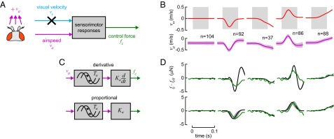
The antenna-mediated airspeed response resembles a proportional controller with a short delay. (A) As in Fig. 3, we eliminated the effect of the visual response by fitting the model to data only during a short period of ms (shaded area in B). (B) We stimulated the fly with several wind gust conditions, shown as in laboratory-frame wind velocity, v_w, with different rates of onset and direction (we omit slower stimulus conditions from view as in Fig. 3). (C) We proposed two controller models with time delays: derivative and proportional (Eqs. 16 and 17). (D) As in Fig. 3, we show the fly-frame input airspeed, v_a (mean ± SD), and the estimated control force output, f_c (mean, jagged green line), computed as in Fig. 4 to permit a visual comparison. The force prediction of the fitted models were computed by simulating the response of the transfer function in Eq. 13 divided by and are plotted in black (smooth line, ± 95% confidence interval in gray). The residual error is higher for the derivative model, and a visual inspection indicates that the poor performance is because it produces a bidirectional reaction to strong gusts, unlike flies’ measured behavior.

Visual Feedback Model.

A full characterization of the slow dynamics of the visual response would require a prohibitively long flight path that was not possible given the length of our tunnel. To circumvent this limitation, we measured short-timescale dynamics with our apparatus and additionally required that long-timescale dynamics be consistent with Charles David’s prior measurements of steady-state wind responses (13). A previous model of a vision-based flight controller by Rohrseitz and Fry (16) posited visual velocity as input and produced groundspeed as an output. Their best-fit model consisted of a two-pole low-pass filter with time delay and airspeed saturation. In terms of physical forces instead of velocities, a controller with similar behavior in quiescent air is a proportional controller of the form

However, this model would show significant error when incorporated in a feedback loop in the presence of wind. Accordingly, we also propose an integral controller,

that winds up the error over time. An integral controller of this form had a correlation with the fly’s behavior almost as strong as that of the two-pole model in ref. 16. We eliminated a derivative model from consideration because it would require a long delay and could not compensate for steady-state wind. To fit the free parameters in these models, we used data from experiments with arista-ablated flies and assumed these animals could not sense airspeed and so had no antenna feedback [Eq. 14 with C_a(s) = 0 was used to predict groundspeed] (Fig. 6A). We fitted data for a period of t_f = 0.4 s because after this time, flies' groundspeeds show a significant negative drift, perhaps because of the aversive effect of the looming darkened end of the wind tunnel (4). The nonlinear regression of flies’ groundspeed responses to visual gusts (Fig. 6B) indicates that the proportional model has a gain μN⋅s⋅m⁻¹ and a time delay of ms (mean ± 95% confidence interval of bootstrap; Fig. S2C), whereas the integral model has μN⋅m⁻¹ and a time delay of ms (Fig. 6 C and D).

Fig. 6.

The visual response resembles an integral controller with a long time delay. (A) To isolate the visual response, we removed the effect of antenna feedback by removing the aristae of the antennae. (B) As in Fig. 5, we stimulated flies with a range of stimuli, shown in laboratory-frame projector velocity, v_p (fitting period shown in gray), and fly-frame visual velocity input, v_v (mean ± SD), considering (C) two proposed models: proportional and integral (Eqs. 18 and 19). The projector velocity is nonzero at the start of the trial because of how the experiment protocol animates the projector to bring flies to the trigger plane (see Trial Protocol in Methods). (D) As in Fig. 3, we show the fly-frame input visual velocity, v_v (mean ± SD), and the estimated control force output, f_c (mean, jagged green line), computed as in Fig. 4, to show the dynamics of the fly’s reactions. The force prediction of the fitted models were computed by simulating the output of the transfer function in Eq. 14 with , divided by , and are plotted in black (smooth line, ± 95% confidence interval in gray).

To address the possibility that arista ablation might affect visual feedback, we performed an additional test of a range of visual gusts on flies with intact antennae (see Fig. S3B for stimulus conditions and responses). In this model-fitting procedure, we included the effect of the proportional antenna response. The gain and delay estimates of both the proportional ( μN⋅s⋅m⁻¹, ms) and integral ( μN⋅m⁻¹, ms) models were at or near the middle of the 95% confidence interval for the arista-ablated flies, indicating that arista ablation has little effect on visual responses.

The Akaike information criterion generated a very weak preference (57%) for the integral model over the proportional model. To use steady-state behavior to differentiate between the models, we considered the thrust force necessary to overcome aerodynamic drag. A feed-forward approach that applies a fixed force based on an a priori estimate of drag is effective only at a specific wind velocity. A more likely possibility is that the fly has a desired groundspeed set point, v_d, that is added to the visual velocity estimate. This error signal, , is fed into the visual controller rather than the visual velocity v_v. Our proportional model operating on this error term would exhibit a large error in the presence of wind because of its low gain. Solving for steady state reveals that the fly’s groundspeed would even go negative (indicative of being blown downwind) when . To compare with observed behavior, we assumed that flies are at steady state at the start of trials in still air and estimated that the set point v_d is equal to the mean of v_v at the start of trials in still air, or approximately 0.10 ms⁻¹. In moving air, a -ms⁻¹ headwind at the start of the wind shutter trials (Fig. 6B, last column), the proportional model for arista-ablated flies predicts a very low groundspeed v_g of only 0.08 ms⁻¹. In contrast, flies’ mean groundspeed was 0.25 ms⁻¹, almost identical to that in the piston trials with zero wind (Mann–Whitney U test, ; a similar result holds for intact flies) and significantly different from 0.08 ms⁻¹ (one-sample t test, ). The integral model, on the other hand, integrates error over time to drive it to zero so that in steady state, in steady wind, regardless of its strength. This corresponds to the flies’ observed behavior. This characteristic of flight first was observed in Drosophila hydei for different wind velocities up to 1 ms⁻¹ (13) and verified for Drosophila melanogaster in our apparatus over the same range. Accordingly, experimental evidence supports the integral model of the fly’s visual feedback controller.

Remarks Concerning the Model.

A block diagram depicting the collective results of the model fitting is shown in Fig. 7A. Its key features are a slower outer loop driven by vision that maintains groundspeed and a faster parallel loop driven by airspeed that stabilizes this controller. We remark that our results also are compatible with the two responses operating in series, rather than in parallel; that is, visual feedback could act to modulate a set-point airspeed. This nested design would be analogous to how the visual system modulates haltere sensitivity (39) and antenna movement (21) to modulate wing-driven rotational motion. Because the predictions are identical for our data, as may be shown by block diagram manipulation, we show a representation of the observed input–output behavior and leave this question to future work.

Fig. 7.

The most parsimonious model of the flies’ forward flight dynamics suggests that the damping effect of the faster antenna response stabilizes the fly’s visual groundspeed controller. (A) A block diagram illustrates components of the identified model. A visual response with a long time delay regulates groundspeed to follow the desired “set point” velocity v_d. A second parallel loop mediated by airspeed feedback from the antennae acts to stabilize the visual regulator through a damping action with low time delay. Passive aerodynamic drag acts in the same direction, with a similar magnitude. (B) We compare groundspeed predictions of the model (dashed, simulated from Eq. 15; for the model of arista-ablated flies) to the mean groundspeeds of flies (solid) in the naturalistic scenario of wind gusts with no laboratory-induced change in visual stimulus. The data and model show reasonable agreement for all tested wind gusts for both intact (black) and arista-ablated (red) flies (Fig. S3 A–C shows all data collected, including responses to visual gusts). (C) When stimulated with a step input in visual velocity, the model of the arista-ablated flies (red, estimate ± 95% parameter confidence interval) is nearly unstable, showing oscillations that resemble those of the arista-ablated flies in Fig. 1D. The instability in the model arises from the long delay and high gain of visual feedback. Adding antenna feedback into the model abolishes the oscillations (black), supporting the hypothesis that its fast damping effect counteracts groundspeed excursions from the desired velocity. (D) A plot of the frequency response of Eq. 13 gives the size of groundspeed error (e_v in A) due to wind disturbance. Adding the integrating visual response reduces the groundspeed error relative to a passive fly (Eq. 12) at low frequencies, at the expense of a nearly unstable resonant peak around 1 Hz. Adding antenna feedback (black) slightly increases the error across most frequencies in exchange for diminishing the resonant peak.

A comparison of the groundspeed predictions of the model with the mean responses of real flies shows reasonable agreement across all tested gusts and visual gusts (Fig. 7B; see Fig. S3 for a plot of all data collected). It is informative to explain how our model is consistent with the results of Fig. 2B. In steady-state forward flight, the role of the integrating controller may be interpreted as finding the necessary forward thrust to compensate for air drag. However, any sudden excursion in airspeed in either direction due to a sudden change in wind speed will induce a compensatory reaction by the antenna response that acts to bring airspeed back to the set point. Thus, the active deceleration of intact flies in the impulsive headwind gust (Fig. 2B) is the result of the antennal response block attempting to maintain the airspeed set point. This response is absent in arista-ablated flies, whose deceleration is the result of only passive aerodynamic drag (Fig. 2C). Because of the differences in delay, the earliest stages of the antenna response occur before visual feedback has an effect on the flies’ motion. A short while later, the visual response begins, and the resulting compensatory overshoot may be observed at ∼200 ms for intact flies in the same pane. Note that this overshoot is absent in response to the gusts presented by the programmed stimulus that cancelled out visual motion (Fig. 4E). In the slower step gust (Fig. 2D), the stronger but slower visual integrator overrides the proportional antenna response and aerodynamic drag to restore most of the original groundspeed within ∼0.5 s.

How Antenna Feedback Might Abolish Groundspeed Variability.

Our identified model exhibits behavior consistent with the hypothesis that the groundspeed oscillations observed in arista-ablated flies (Fig. 1D) are the result of feedback instability. When simulated in closed loop with a step input in projector velocity similar to the visual stimulus preceding all trials (Trial Protocol), our model of arista-ablated flies exhibits similar groundspeed oscillations (Fig. 7C, red line). The model for arista-ablated flies has a gain margin of only 1.6 (the 95% confidence interval ranges from 6.8 to an unstable 0.8) and a phase margin of 25° (55° to an unstable −16°) when the loop is broken at v_v (see Bode plot in Fig. S3D). Our limited tunnel length gave only a rough estimate of the visual feedback parameters, but the detail is sufficient to conclude that the delay is long enough and the gain high enough that there is near-instability across most of the uncertainty interval. Our time delay closely matches a previous estimate of 80 ms (16). If antennal feedback is added, oscillations in the model are abolished because of the damping effect of the antenna-mediated response (Fig. 7C, black line). This raises the gain and phase margins to 3.0 (11.9–1.4) and 56° (77°–27°), respectively. We neglected antenna and drag model uncertainty in these stability margin calculations because they are small relative to visual uncertainty. Our results are consistent with the view that the antennal response provides damping, a role equivalent to the derivative term in the proportional-integral-derivative controllers ubiquitous in engineering (26). In both cases, the effect is to reduce phase delay at the unity–gain crossover frequency, increasing stability and robustness to parameter uncertainty. By providing robustness, the antenna response might enable the fly’s flight controller to perform acceptably despite variations in visual scene intensity, obstacle distance, contrast, temperature, or muscular fatigue. Whereas the model reported here provides a parsimonious explanation for the observed behavior, the antennae play many roles in flight that might be compromised by our experimental ablations. Therefore, our conclusions regarding the precise role of the antennae must remain speculative until further experiments with less disruptive manipulations can be performed.

Discussion

The results reported here provide insight into how flies combine information from their visual system and their antennae to regulate forward flight speed. Although vision may provide an estimate of groundspeed in the presence of a steady wind, it does so with a functionally significant delay of ∼50–100 ms. Mechanoreceptors on the antennae, on the other hand, cannot measure groundspeed directly, but our results suggest they can detect changes in airspeed more quickly (within ∼20 ms). They use this information to add active damping that counteracts unstable oscillations, in exchange for increasing the effect of sudden wind disturbances. Although prior work demonstrates that the antennae may play many roles in flight (18, 23–25), their ability to provide stability for the visual groundspeed controller was not identified previously. Damping also might be achieved by using passive components such as a long abdomen or dangling legs, but this would increase energy costs during flight and impede sudden maneuvers. By using a sensory-driven response, the fly can increase damping only when required. This control strategy might aid in the design of small autonomous flying vehicles, whose visual autopilots are similarly bandwidth limited because of noise or limits to available onboard computation (40, 41).

In interpreting our results, it is critical to note that although the brief wind gusts we used were useful for probing the architecture of the flight control system, such stimuli may be uncommon in the natural world. Airflow through the plant canopy inhabited by Drosophila typically is turbulent, exhibiting a characteristic flow pattern in which brief transients, similar to those generated by the piston, are statistically likely to be much weaker than those of longer duration (42). Wind speed measurements in and above cornfields (43) and deciduous forests (42, 44) indicate that wind speed amplitude decreases as frequency increases from 0.1 to 20 Hz, resembling the theoretical prediction of an power spectrum (42). Hence, high-frequency gusts, such as our air piston gusts, are weak in natural environments and likely would induce only small perturbations in the wind direction. A visual response that operates like an integrator, as suggested by our results, would be ideally suited to compensate for the stronger, low-frequency disturbances that dominate the energy in turbulent natural flows (Fig. 7D).

Active damping is thought to play a significant role in stabilizing the dynamics of insect locomotion (45). In running cockroaches, antenna feedback used in wall following provides a derivative term that adds a stabilizing damping effect (46). In flying insects, active damping augments the passive rotational damping induced by aerodynamic wing drag (32, 36, 47–49). It previously was argued that damping induced by compensatory responses mediated by the halteres might stabilize rotatory feedback from vision (48), which has a longer delay (50). Hawk moths exhibit another possible example of this principle in which fast antennal feedback adds linearly to slower visual feedback to regulate the stabilizing motion of the abdomen during hovering flight (24, 51). In the present study, we have shown that flies use this same principle in the context of translational flight control, which involves different constraints. In contrast to rotatory motion, the optic flow produced by translatory motion varies in magnitude with the distance to obstacles (52). Bees (53) and flies (13) accelerate in a gradually widening corridor, consistent with an angular optic flow regulator. A narrower corridor or a closer obstacle produces greater optic flow for a given groundspeed and so is equivalent to a higher gain in the visual feedback loop. Because the absolute distance to an object is not easily measured (52, 54), there is an intrinsic inaccuracy in visual estimates of translational velocity. Our model suggests that the high gain induced by nearby obstacles might lead to instability when combined with the long delay of visual feedback. To our knowledge, the ramifications of this visual uncertainty were not considered previously in the context of feedback dynamics. Our results suggest that the damping effect provided by the antennae may aid the fly by stabilizing flight in confined spaces.

References

- 1.Randall DJ, Burggren WW, French K, Eckert R. Eckert Animal Physiology: Mechanisms and Adaptations. New York: Freeman; 2002. [Google Scholar]
- 2.Taylor GK, Krapp HG. In: Sensory Systems and Flight Stability: What Do Insects Measure and Why? Insect Mechanics and Control, Advances in Insect Physiology. Casas J, Simpson SJ, editors. Vol 34. New York: Academic; 2007. pp. 231–316. [Google Scholar]
- 3.Land MF, Collett TS. Chasing behavior of houseflies. J Comp Physiol A Neuroethol Sens Neural Behav Physiol. 1974;89(4):331–357. [Google Scholar]
- 4.Card G, Dickinson MH. Performance trade-offs in the flight initiation of Drosophila. J Exp Biol. 2008;211(3):341–353. doi: 10.1242/jeb.012682. [DOI] [PubMed] [Google Scholar]
- 5.Deng X, Schenato L, Wu WC, Sastry SS. Flapping flight for biomimetic robotic insects: Part I—system modeling. IEEE Trans Robot. 2006;22(4):776–788. [Google Scholar]
- 6.Dickson WB, Straw AD, Dickinson MH. Integrative model of Drosophila flight. AIAA J. 2008;46(9):2150–2164. [Google Scholar]
- 7.Lindemann JP, Kern R, van Hateren JH, Ritter H, Egelhaaf M. On the computations analyzing natural optic flow: Quantitative model analysis of the blowfly motion vision pathway. J Neurosci. 2005;25(27):6435–6448. doi: 10.1523/JNEUROSCI.1132-05.2005. [DOI] [PMC free article] [PubMed] [Google Scholar]
- 8.Ristroph L, et al. Discovering the flight autostabilizer of fruit flies by inducing aerial stumbles. Proc Natl Acad Sci USA. 2010;107(11):4820–4824. doi: 10.1073/pnas.1000615107. [DOI] [PMC free article] [PubMed] [Google Scholar]
- 9.Stewart FJ, Baker DA, Webb B. A model of visual-olfactory integration for odour localisation in free-flying fruit flies. J Exp Biol. 2010;213(11):1886–1900. doi: 10.1242/jeb.026526. [DOI] [PubMed] [Google Scholar]
- 10.Schilstra C, Hateren JH. Blowfly flight and optic flow. I. Thorax kinematics and flight dynamics. J Exp Biol. 1999;202(11):1481–1490. doi: 10.1242/jeb.202.11.1481. [DOI] [PubMed] [Google Scholar]
- 11.Tammero LF, Dickinson MH. The influence of visual landscape on the free flight behavior of the fruit fly Drosophila melanogaster. J Exp Biol. 2002;205(3):327–343. doi: 10.1242/jeb.205.3.327. [DOI] [PubMed] [Google Scholar]
- 12.Fry SN, Sayaman R, Dickinson MH. The aerodynamics of free-flight maneuvers in Drosophila. Science. 2003;300(5618):495–498. doi: 10.1126/science.1081944. [DOI] [PubMed] [Google Scholar]
- 13.David CT. Compensation for height in the control of groundspeed by Drosophila in a new, ‘barber’s pole’ wind tunnel. J Comp Physiol A Neuroethol Sens Neural Behav Physiol. 1982;147(4):485–493. [Google Scholar]
- 14.Kennedy JS. The visual responses of flying mosquitos. Proc Zoological Soc London. 1940;A109(4):221–242. [Google Scholar]
- 15.Fry SN, Rohrseitz N, Straw AD, Dickinson MH. Visual control of flight speed in Drosophila melanogaster. J Exp Biol. 2009;212(8):1120–1130. doi: 10.1242/jeb.020768. [DOI] [PubMed] [Google Scholar]
- 16.Rohrseitz N, Fry SN. Behavioural system identification of visual flight speed control in Drosophila melanogaster. J R Soc Interface. 2011;8(55):171–185. doi: 10.1098/rsif.2010.0225. [DOI] [PMC free article] [PubMed] [Google Scholar]
- 17.Hollick FSJ. The flight of the dipterous fly Muscina stabulans Fallen. Philos Trans R Soc Lond B Biol Sci. 1940;230(572):357–390. [Google Scholar]
- 18.Burkhardt D, Gewecke M. Mechanoreception in Arthropoda: The chain from stimulus to behavioral pattern. Cold Spring Harb Symp Quant Biol. 1965;30:601–614. doi: 10.1101/sqb.1965.030.01.058. [DOI] [PubMed] [Google Scholar]
- 19.Gewecke M, Schlegel P. The vibrations of the antenna and their significance for flight control in the blow fly Calliphora erythrocephala. J Comp Physiol A Neuroethol Sens Neural Behav Physiol. 1970;67:325–362. [Google Scholar]
- 20.Budick SA, Reiser MB, Dickinson MH. The role of visual and mechanosensory cues in structuring forward flight in Drosophila melanogaster. J Exp Biol. 2007;210(23):4092–4103. doi: 10.1242/jeb.006502. [DOI] [PubMed] [Google Scholar]
- 21.Mamiya A, Straw AD, Tómasson E, Dickinson MH. Active and passive antennal movements during visually guided steering in flying Drosophila. J Neurosci. 2011;31(18):6900–6914. doi: 10.1523/JNEUROSCI.0498-11.2011. [DOI] [PMC free article] [PubMed] [Google Scholar]
- 22.Yorozu S, et al. Distinct sensory representations of wind and near-field sound in the Drosophila brain. Nature. 2009;458(7235):201–205. doi: 10.1038/nature07843. [DOI] [PMC free article] [PubMed] [Google Scholar]
- 23.Sane SP, Dieudonné A, Willis MA, Daniel TL. Antennal mechanosensors mediate flight control in moths. Science. 2007;315(5813):863–866. doi: 10.1126/science.1133598. [DOI] [PubMed] [Google Scholar]
- 24.Hinterwirth AJ, Daniel TL. Antennae in the hawkmoth Manduca sexta (Lepidoptera, Sphingidae) mediate abdominal flexion in response to mechanical stimuli. J Comp Physiol A Neuroethol Sens Neural Behav Physiol. 2010;196(12):947–956. doi: 10.1007/s00359-010-0578-5. [DOI] [PubMed] [Google Scholar]
- 25.Taylor GJ, Luu T, Ball D, Srinivasan MV. Vision and air flow combine to streamline flying honeybees. Sci Rep. 2013;3:2614. doi: 10.1038/srep02614. [DOI] [PMC free article] [PubMed] [Google Scholar]
- 26.Astrom KJ, Murray RM. Feedback Systems: An Introduction for Scientists and Engineers. Princeton, NJ: Princeton Univ Press; 2008. [Google Scholar]
- 27.Budick SA, Dickinson MH. Free-flight responses of Drosophila melanogaster to attractive odors. J Exp Biol. 2006;209(15):3001–3017. doi: 10.1242/jeb.02305. [DOI] [PubMed] [Google Scholar]
- 28.Straw AD, Lee S, Dickinson MH. Visual control of altitude in flying Drosophila. Curr Biol. 2010;20(17):1550–1556. doi: 10.1016/j.cub.2010.07.025. [DOI] [PubMed] [Google Scholar]
- 29.Straw AD, Branson K, Neumann TR, Dickinson MH. Multi-camera realtime 3D tracking of multiple flying animals. J R Soc Interface. 2010;8(56):395–409. doi: 10.1098/rsif.2010.0230. [DOI] [PMC free article] [PubMed] [Google Scholar]
- 30.Straw AD. Vision egg: An open-source library for realtime visual stimulus generation. Front Neuroinform. 2008;2:4. doi: 10.3389/neuro.11.004.2008. [DOI] [PMC free article] [PubMed] [Google Scholar]
- 31.David CT. The relationship between body angle and flight speed in free-flying Drosophila. Physiol Entomol. 1978;3(3):191–195. [Google Scholar]
- 32.Dickson WB, Polidoro P, Tanner MM, Dickinson MH. A linear systems analysis of the yaw dynamics of a dynamically scaled insect model. J Exp Biol. 2010;213(17):3047–3061. doi: 10.1242/jeb.042978. [DOI] [PubMed] [Google Scholar]
- 33.Bergou AJ, Ristroph L, Guckenheimer J, Cohen I, Wang ZJ. Fruit flies modulate passive wing pitching to generate in-flight turns. Phys Rev Lett. 2010;104(14):148101. doi: 10.1103/PhysRevLett.104.148101. [DOI] [PubMed] [Google Scholar]
- 34.Vogel S. Flight in Drosophila: I. Flight performance of tethered flies. J Exp Biol. 1966;44(1):567–578. [Google Scholar]
- 35.Teoh ZE, et al. 2012. A hovering flapping-wing microrobot with altitude control and passive upright stability. In IROS (IEEE), pp 3209–3216.
- 36.Hesselberg T, Lehmann F-O. Turning behaviour depends on frictional damping in the fruit fly Drosophila. J Exp Biol. 2007;210(24):4319–4334. doi: 10.1242/jeb.010389. [DOI] [PubMed] [Google Scholar]
- 37.Ljung L. System Identification. Upper Saddle River, NJ: Prentice Hall; 1999. [Google Scholar]
- 38.Webb B, Reeve R. Reafferent or redundant: Integration of phonotaxis and optomotor behavior in crickets and robots. Adapt Behav. 2003;11(3):137–158. [Google Scholar]
- 39.Chan WP, Prete F, Dickinson MH. Visual input to the efferent control system of a fly’s “gyroscope.”. Science. 1998;280(5361):289–292. doi: 10.1126/science.280.5361.289. [DOI] [PubMed] [Google Scholar]
- 40.Zufferey J-C, Floreano D. Fly-inspired visual steering of an ultralight indoor aircraft. IEEE Trans Robot. 2006;22(1):137–146. [Google Scholar]
- 41.Ma KY, Chirarattananon P, Fuller SB, Wood RJ. Controlled flight of a biologically inspired, insect-scale robot. Science. 2013;340(6132):603–607. doi: 10.1126/science.1231806. [DOI] [PubMed] [Google Scholar]
- 42.Kaimal JC, Finnigan JJ. Atmospheric Boundary Layer Flows: Their Structure and Measurement. New York: Oxford Univ Press; 1994. [Google Scholar]
- 43.Wilson JD, Ward DP, Thurtell GW, Kidd GE. Statistics of atmospheric turbulence within and above a corn canopy. Boundary-Layer Meteorol. 1982;24(4):495–519. [Google Scholar]
- 44.Baldocci DD, Meyers TP. A spectral and lag-correlation analysis of turbulence in a deciduous forest canopy. Boundary-Layer Meteorol. 1988;45(1-2):31–58. [Google Scholar]
- 45.Hedrick TL. Damping in flapping flight and its implications for manoeuvring, scaling and evolution. J Exp Biol. 2011;214(24):4073–4081. doi: 10.1242/jeb.047001. [DOI] [PubMed] [Google Scholar]
- 46.Cowan NJ, Lee J, Full RJ. Task-level control of rapid wall following in the American cockroach. J Exp Biol. 2006;209(9):1617–1629. doi: 10.1242/jeb.02166. [DOI] [PubMed] [Google Scholar]
- 47.Cheng B, Deng X. Translational and rotational damping of flapping flight and its dynamics and stability at hovering. IEEE Trans Robot. 2011;27(5):849–864. [Google Scholar]
- 48.Elzinga MJ, Dickson WB, Dickinson MH. The influence of sensory delay on the yaw dynamics of a flapping insect. J R Soc Interface. 2012;9(72):1685–1696. doi: 10.1098/rsif.2011.0699. [DOI] [PMC free article] [PubMed] [Google Scholar]
- 49.Hedrick TL, Cheng B, Deng X. Wingbeat time and the scaling of passive rotational damping in flapping flight. Science. 2009;324(5924):252–255. doi: 10.1126/science.1168431. [DOI] [PubMed] [Google Scholar]
- 50.Sherman A, Dickinson MH. A comparison of visual and haltere-mediated equilibrium reflexes in the fruit fly Drosophila melanogaster. J Exp Biol. 2003;206(2):295–302. doi: 10.1242/jeb.00075. [DOI] [PubMed] [Google Scholar]
- 51.Dyhr JP, Morgansen KA, Daniel TL, Cowan NJ. Flexible strategies for flight control: An active role for the abdomen. J Exp Biol. 2013;216(9):1523–1536. doi: 10.1242/jeb.077644. [DOI] [PubMed] [Google Scholar]
- 52.Koenderink JJ. Optic flow. Vision Res. 1986;26(1):161–179. doi: 10.1016/0042-6989(86)90078-7. [DOI] [PubMed] [Google Scholar]
- 53.Srinivasan MV, Zhang S, Lehrer M, Collett T. Honeybee navigation en route to the goal: Visual flight control and odometry. J Exp Biol. 1996;199(1):237–244. doi: 10.1242/jeb.199.1.237. [DOI] [PubMed] [Google Scholar]
- 54.Han S, Censi A, Straw AD, Murray RM. 2010. A bio-plausible design for visual pose stabilization. In IROS (IEEE), pp 5679–5686.
Associated Data
This section collects any data citations, data availability statements, or supplementary materials included in this article.