

Abstract
Introduction:
Self-regulation, a key component of the addiction process, has been challenging to model precisely in smoking cessation settings, largely due to the limitations of traditional methodological approaches in measuring behavior over time. However, increased availability of intensive longitudinal data (ILD) measured through ecological momentary assessment facilitates the novel use of an engineering modeling approach to better understand self-regulation.
Methods:
Dynamical systems modeling is a mature engineering methodology that can represent smoking cessation as a self-regulation process. This article shows how a dynamical systems approach effectively captures the reciprocal relationship between day-to-day changes in craving and smoking. Models are estimated using ILD from a smoking cessation randomized clinical trial.
Results:
A system of low-order differential equations is presented that models cessation as a self-regulatory process. It explains 87.32% and 89.16% of the variance observed in craving and smoking levels, respectively, for an active treatment group and 62.25% and 84.12% of the variance in a control group. The models quantify the initial increase and subsequent gradual decrease in craving occurring postquit as well as the dramatic quit-induced smoking reduction and postquit smoking resumption observed in both groups. Comparing the estimated parameters for the group models suggests that active treatment facilitates craving reduction and slows postquit smoking resumption.
Conclusions:
This article illustrates that dynamical systems modeling can effectively leverage ILD in order to understand self-regulation within smoking cessation. Such models quantify group-level dynamic responses in smoking cessation and can inform the development of more effective interventions in the future.
INTRODUCTION
The chronic, relapsing nature of cigarette smoking and its related health and economic impacts makes smoking a significant public health issue (Fiore et al., 2008). If more effective smoking cessation interventions are to be designed, it is important to better understand the process of cessation (Shiffman, 2006). Supporting a long-term goal of more effective, personalized interventions, emerging technologies and analytical methods are being employed in pursuit of more comprehensive descriptions of smoking behavior change.
Self-regulation theory has been of particular interest in describing smoking behavior, postulating that smoking is done to correct deviations from a “normal” level of some variable, such as blood nicotine or affect levels (i.e., achieve homeostasis; Carver & Scheier, 1998; Solomon, 1977; Solomon & Corbit, 1974; Velicer, Redding, Richmond, Greeley, & Swift, 1992). Changes in smoking rates are said to be directly proportional to the difference between the normal level of the regulated variable and its actual level at some time (Velicer et al., 1992).
Historically, precise modeling of self-regulation has been met with limited success. This is largely the result of difficulty measuring behavior frequently over time in the prepersonal computing era and the traditional emphasis on statistical methodologies that are static in nature (Riley et al., 2011). However, technological advances (e.g., handheld computers) mean that dynamic behaviors can be effectively and efficiently assessed repeatedly over time, providing intensive longitudinal data (ILD; Walls & Schafer, 2006). These technologies enable cost-effective measurement of behavior in real time in the real world (i.e., outside of laboratory environments), providing more informative data (i.e., via data collection by ecological momentary assessment [EMA] protocols; Shiffman, Stone, & Hufford, 2008).
The advent of behavioral ILD has led to modeling efforts that aim to characterize dynamic phenomena within behavioral, social, and public health settings (Boker, 2012; Boker & Nesselroade, 2002; Ionides, Bretó, & King, 2006; Rivera, 2012; Rivera, Pew, & Collins, 2007; Tan, Shiyko, Li, Li, & Dierker, 2012; Trail et al., in press). The result includes novel descriptions of time-varying predictors of substance use (Chandra, Scharf, & Shiffman, 2011; Galea, Hall, & Kaplan, 2009; Samanta, 2011; Shiyko, Lanza, Tan, Li, & Shiffman, 2012; Timms, Rivera, Collins, & Piper, 2012), pain management (Deshpande, Nandola, Rivera, & Younger, 2011), and disease transmission within populations (Bhadra et al., 2011; Ionides et al., 2006). Increased availability of ILD also allows use of an engineering analytical approach to study self-regulation within smoking (Rivera 2012; Timms et al., 2012). Furthermore, constructing models of self-regulated smoking behaviors using an engineering approach is motivated by the fact that similar models describing smoking as a regulation-free process do not comprehensively describe the interrelationship between smoking and craving that is observed in smoking cessation clinical trial ILD (Timms et al., 2012).
Traditionally applied within engineering settings, dynamical systems modeling (referred to as dynamic modeling) can be used to describe how outcomes of interest (e.g., smoking) respond to changes in exogenous and predictor variables (e.g., quit attempt and craving, respectively). System identification involves a set of techniques within dynamic modeling that deals with methods to produce empirical dynamic models from data (Ljung, 1999). Together, dynamic modeling and system identification use ordinary differential equations (ODEs) to parsimoniously and comprehensively describe processes of change. Commonly used in engineering to describe change within physical systems (Ogunnaike & Ray, 1994), ODEs have also been used to describe the dynamics in behavior (Boker, 2012; Boker & Nesselroade, 2002). The approach considered in this work similarly relies on ODEs, but employs an input–output perspective, meaning dynamic models describe how changes in inputs to a process lead to changes in outputs of that process. In behavioral health contexts, input variables correspond to predictor variables that may or may not be independent (e.g., a quit attempt and smoking, respectively) and output variables correspond to outcomes or dependent variable responses (e.g., craving; Trail et al., in press). Dynamic models are able to quantify not only the net effect a change in a predictor variable has on an outcome variable but also how quickly the response occurs, whether the response is oscillatory, and more (Ogunnaike & Ray, 1994).
Dynamic modeling is an appealing way to model smoking behavior change because it is often used by engineers to characterize regulatory (feedback) processes. Dynamic models based on ILD collected via EMA protocols can provide a more rigorous and parsimonious description of the self-regulatory dynamics of smoking behaviors in real-world environments. An understanding of self-regulatory dynamics is of considerable interest as such estimated expressions can shed light on the nature of craving regulation. This, in turn, may provide insight into the craving process that leads to cessation relapse, as craving and craving suppression have been strongly implicated in cessation success (Bolt, Piper, Theobald, & Baker, 2012; McCarthy et al., 2008b; Piper et al., 2008; Timms et al., 2012). This insight may help inform development of more effective smoking cessation interventions in the future (Riley et al., 2011; Timms, Rivera, Collins, & Piper, 2013).
This article aims to illustrate the benefits of dynamic modeling by mathematically modeling day-to-day changes in the self-regulatory relationship between Current Craving (average daily craving level) and CPD (total number of cigarettes smoked per day) during a quit attempt. These models are developed using group average ILD from a University of Wisconsin clinical trial; this facilitates characterization of the fundamental self-regulation process over a critical cessation timeframe, beginning 1 week prior to and ending approximately 1 month after the target quit date. In the Methods section, details of the University of Wisconsin clinical trial data, the self-regulation model, and model estimation procedures are presented. Empirical dynamic models estimated for the clinical trial’s active and placebo treatment groups are then contrasted and explained. Finally, future use of this modeling approach, connections between self-regulation models and ongoing questions in cessation research, and implications of the findings for intervention development are briefly discussed.
METHODS
Clinical Trial Data
The EMA data analyzed in this article comes from a University of Wisconsin Center for Tobacco Research and Intervention randomized placebo-controlled clinical trial of the effects of bupropion SR and counseling on smoking cessation (McCarthy et al., 2008a). Study participants were randomly assigned to one of four experimental conditions. This article focuses on one active treatment and the no treatment group. In the active treatment group, 100 participants received both active bupropion and counseling (the “AC” group): 46.0% female; 1.0% Hispanic, 90.0% White, 7.0% Black, and 3.0% other; mean age, 36.9±11.5 years; mean baseline Fagerström Test for Nicotine Dependence [FTND] score, 5.0±2.5. These participants took 150mg/day of bupropion twice a day, from 1 week pretarget quit day to 8 weeks postquit, with the appropriate 3-day ramp-up period of only 150mg/day. In-person counseling consisted of eight sessions and covered topics such as problem solving, support, coping, and motivation. In the no treatment condition, 100 participants received a placebo drug, taken on the same schedule as the active medication, and no counseling (“PNc” group): 54.0% female; 0.0% Hispanic, 92.0% White, 5.0% Black, and 3.0% other; mean age, 39.2±11.4 years; mean baseline score, 5.1±2.1 (McCarthy et al., 2008a).
Data were collected using personal digital assistants for 2 weeks prior to and 4 weeks following the target quit date. This article draws from Evening Reports (ERs), self-reports completed daily prior to going to bed (McCarthy et al., 2008a). ERs included items from the Wisconsin Smoking Withdrawal Scale (Welsch et al., 1999) and the Positive and Negative Affect Scale (Watson, Clark, & Tellegen, 1988). Current Craving is defined as the sum of Urge (“Urge(s) to smoke?”), Cigonmind (“Cigarettes on my mind?”), Thinksmk (“Thinking about smoking a lot?”), and Bother (“Bothered by desire to smoke?”), each assessed as “Since Last ER on Average” on a 10-point Likert scale (1–11, No!! … Yes!!). CPD was also measured (“Since Last ER—Total cigarettes smoked since the last evening report?”).
Although single subject (idiographic) models could be examined (see Timms et al. 2012, 2013 for example), group average data were the focus of this analysis. This was done primarily to characterize self-regulatory dynamics within two populations, which can also provide insight into treatment condition effects.
Self-Regulation Model
Figure 1 is a block diagram, typically used by engineers, which describes the self-regulatory relationship between Current Craving and CPD from an input–output perspective. The overall self-regulation system is composed of three individual input–output processes, depicted as blocks in Figure 1. These processes are related in a way that suggests cigarettes are smoked in an attempt to maintain a smoker’s average prequit craving level, Baseline Craving Level. Because the system aims to sustain Current Craving at a level equal to Baseline Craving Level, Current Craving is said to be the primary output of the overall self-regulation system, as is depicted on the right side of Figure 1. A quit attempt significantly perturbs the overall regulatory process.
Figure 1.

Block diagram depicting the relation between Current Craving and CPD as a self-regulatory process. Current Craving is the variable representing the average craving level for each day in the time period examined. CPD is the variable representing the total number of cigarettes smoked each day in the time period examined. Baseline Craving Level is a constant value equal to the average prequit daily craving level. For each day, Daily Craving Difference equals the difference between Baseline Craving Level and the value of Current Craving for that day. Quit is the variable representing the attempt to quit smoking (Quit = 0 prior to the target quit day and Quit = 1 beginning on the target quit day).
Examining Figure 1 from right to left, Current Craving is the direct result of total daily smoking, CPD. The manner in which day-to-day changes in CPD lead to day-to-day changes in Current Craving is described by the Craving Generation Process (depicted as a block in Figure 1). In other words, CPD is the “input” to the Craving Generation Process and Current Craving is the “output.” CPD is the sum of the outputs of two processes: the Quit Attempt Process and Craving Self-Regulator (also depicted as blocks in Figure 1). The Quit Attempt Process reflects the extent to which an attempt to quit smoking influences CPD. The Craving Self-Regulator represents how Daily Craving Difference influences CPD. The value of Daily Craving Difference for each day is the difference between Baseline Craving Level, a constant value, and the value of Current Craving for that day. In other words, the Craving Self-Regulator produces changes in CPD in order to minimize the difference between Baseline Craving Level and Current Craving. This process reflects a biological or psychological homeostatic mechanism that promotes smoking in an attempt to maintain Current Craving at a level near Baseline Craving Level. Comparing Figure 1 to the representation of self-regulating behavior presented in Carver and Scheier (1998), the Craving Generation Process is equivalent to the “Effect on Environment” process and the Craving Self-Regulator is equivalent to “Behavior.”
The system in Figure 1 indicates that Current Craving and CPD are interrelated because changes in Current Craving lead to changes in CPD, and these changes in CPD lead to further changes in Current Craving, and so on. It follows that on average, a change in either Current Craving or CPD will result in a change in the other.
Dynamic models of the Craving Generation Process, Quit Attempt Process, and Craving Self-Regulator (the process blocks in Figure 1) are ODEs that are originally in variable form. With ILD—specifically, data for Quit, Current Craving, and CPD—mathematical expressions that represent the process blocks in Figure 1 can be estimated using regression routines from system identification. The result is compact empirical mathematical functions with estimated parameters that describe the features of cessation dynamics (Ogunnaike & Ray, 1994).
Model Estimation
Dynamic models parsimoniously represent the dynamics of a system using ODEs. These differential equations feature an output variable that is a function of time (e.g., y(t)) and its derivative (e.g.,  ). The derivative describes the output variable’s rate of change.
An example of an ODE that describes simple (first order) dynamics is:
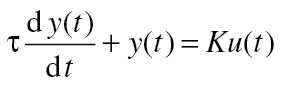 |
(1) |
where u(t) is the input variable and y(t) is the output variable. K is the gain, which quantifies the net change in the output variable per unit change in the input variable. τ is the time constant (in units of time), which quantifies the speed of the response. For first-order ODEs, like Equation 1, τ represents how long it takes for approximately 63% of the total output variable response to be reached, given a step change from 0 to 1 in the input variable.
To interpret Equation 1, consider the Craving Generation Process in Figure 1 as an example: the input is CPD and the output is Current Craving. Equation 1 states that the level of Current Craving at some given time (the y value at t = some specific time point) is related to the rate at which Current Craving changes over time ( ) as well as the level of the input CPD (u(t) at that time). Equation 1 is fit to Current Craving and CPD EMA data, resulting in estimates for K and τ. These estimated parameters contain information on how Current Craving changes over time in response to changes in CPD.
Figure 2 is a plot of dynamics that can be represented by Equation 1 and is not meant to depict any specific dynamics related to smoking or behavior. If complex dynamics (e.g., oscillation) cannot be fully represented by only the parameters K and τ—that is, a first-order ODE insufficiently represents observed dynamics—then higher order ODE structures can be used to describe more complicated dynamics. Notably, higher order ODE structures can feature a system zero, τa, which describes response shape, and a damping coefficient, which describes oscillation (Ogunnaike & Ray, 1994).
Figure 2.

Response of an output variable, y(t), to an input variable, u(t), which changes in value at time 0. The change in the input variable results in changes in the output variable. The characteristics of the output variable’s response to the change in the input variable, such as the magnitude of the output variable change and how quickly this occurs, is defined by Equation 1, a first-order (simple) ODE, and the values of gain K and time constant τ.
Because ODEs include rates of change (the derivative term) and do not explicitly include time as an independent variable, ODEs significantly differ from more common behavioral science modeling methods, such as linear growth curve modeling (Trail et al., in press). Consequently, the parameters in dynamic models require distinct interpretations compared to parameters in linear growth curve and other more traditional analytical methods. Table 1 summarizes the interpretations of the gain, time constant, and system zero parameters.
Table 1.
Summary of the Interpretations of Key Parameters in Dynamic Modeling
| Parameter | Interpretation | Units | Example in terms of the Craving Generation Process |
|---|---|---|---|
| Gain, K | Magnitude of change in an output variable per unit change of an input variable | Output variable units/ input variable units | K 1, Craving generation process gain: the net change in current craving due to a one cigarette increase in CPD |
| Time constant, τ | The speed at which an output variable changes in response to a change in an input variable | Time (e.g., days) | τ1, Craving generation process time constant: reflects the speed at which current craving changes in response to a change in CPD |
| System zero, τa | A negative value indicates inverse response, which refers to an output variable whose initial change is in a direction opposite that of the net change | None | τa, Craving generation process’ system zero: a negative τa value indicates inverse response in current craving, that is, a change in CPD leads to an immediate increase in current craving, which subsequently settles to new, lower level |
In this article, Prediction-Error Methods (PEM) were used to fit a continuous-time model (e.g., Equation 1) to sampled data. PEM and other parameter estimation techniques from system identification are based in well-known regression routines that are extensively documented in statistical literature (Ljung, 1999), preinstalled in software packages such as MATLAB (Ljung, 2003), and utilized by behavioral scientists in more common modeling methods. Consequently, the statistical properties of the parameter estimates presented in this article align with the properties of parameter estimates obtained in more traditional modeling approaches (Ljung, 1999). A comprehensive introduction to parameter estimation from system identification is found in Ljung (1999). Additional details of the connection between continuous-time models and sampled data, the parameter estimation computations, and the software tools used are found in the Supplementary Material; the following describes essential components of estimation. PEM routines in MATLAB, which are part of a precoded, flexible interface for broadly applicable parameter estimation and model evaluation (Ljung, 2012; MathWorks, 2013) were used for parameter estimation here. MATLAB’s PEM command requires input data, output data, and equation structure (e.g., first-order ODE, see Equation 1; Ljung, 2012). By specifying the appropriate input and output data, ODEs of the three processes in the self-regulation system—that is, the blocks in Figure 1—can be obtained: the mathematical function describing the Craving Generation Process was estimated as a single-input–single-output system where CPD is the input and Current Craving the output; the mathematical functions describing the Quit Attempt Process and Craving Self-Regulator processes were estimated as a two-input–one-output system, where Quit and Daily Craving Difference (= Baseline Craving Level − Current Craving) were the inputs and CPD the output (see Figure 1). Quit is an exogenous, independent input variable that corresponds to the transition from not attempting to quit smoking (Quit = 0) to attempting to quit (Quit = 1, beginning on the target quit date). It is treated as an exogenous variable here because participants were instructed to quit on a target date by study administrators (McCarthy et al., 2008a).
This research involved estimation of candidate sets of differential equations using different combinations of ODE structures to describe the three dynamic processes that make up the self-regulation system. Each set of estimated models were then used in a simulation. In this context, simulations offer a means to evaluate how well a candidate set of model estimates can together describe the observed ILD, even though the three ODEs were estimated in two separate steps (estimation of the Craving Generation Process function, followed by estimation of the Quit Attempt Process and Craving Self-Regulator functions). For example, one set of candidate ODE expressions were estimated that employed Equation 1 to describe the Craving Generation Process, Craving Self-Regulator, and Quit Attempt Process. For simulation, these three estimated expressions were related according to the structure depicted in Figure 1 in Simulink, MATLAB’s simulation environment. The simulation resulted in predicted Current Craving and CPD responses to a quit attempt, where the predicted response dynamics were determined by the estimated models. A second set of differential equations were then estimated that employed a more complex ODE structure to describe the Craving Generation Process, and the simpler ODE structure in Equation 1 to describe the Craving Self-Regulator and Quit Attempt Process. The predicted responses of Current Craving and CPD to a quit attempt were then obtained through simulation using this second set of estimated models. This estimation–simulation procedure was repeated using different combinations of low-order (relatively simple) ODE structures and for both the AC and PNc datasets.
Quantification of how well the overall model—that is, the Current Craving and CPD predictions obtained through simulation—fit the ILD was calculated according to the following goodness-of-fit criterion:
 |
(2) |
where y(t) is measured output data,  is the average of the measured output data,
  is the model’s predicted output, and ||·||2 indicates the two-norm (the square root of the sum of the squared vector elements). The simulated Current Craving and CPD responses were also plotted, allowing visual determination of whether a candidate set of estimated ODE expressions adequately represented the observed dynamics. Through visual comparison and calculation of the goodness-of-fit value, the set of estimated expressions that best described the self-regulated smoking behavior change could be determined.
Generally, engineers develop dynamic models with the aim of describing how a system responds to changes in input variables over time. Engineers typically do not use this approach to formally confirm or reject hypotheses. Consequently, this article’s primary intent is to characterize self-regulatory dynamics during cessation as captured on the group level. In this case, EMA data are available for two different treatment groups, meaning models can be developed for each group. Although dynamic models are not typically used in hypothesis testing, it is possible to compare the 99% CIs between the groups to draw preliminary conclusions about group differences. The confidence intervals—which are time varying—are primarily examined for such analysis because they reflect the parameter estimates in combination, and the overall response of a dynamic model is more important than any single set of parameter estimates.
RESULTS
Table 2 contains the parameter estimates for the AC and PNc estimated models. These estimates correspond to the empirical models that most accurately describe the dynamics of the observed Current Craving–CPD interrelationship during a quit attempt; this accuracy is supported by the high goodness-of-fit values (87.32% and 62.25% of variance in Current Craving for the AC and PNc groups, respectively, and 89.16% and 84.12% of variance in CPD for the AC and PNc groups, respectively), which are achieved with low-order (parsimonious) expressions, suggesting the models are reflecting the true process dynamics and are not over-fitting the data.
Table 2.
Goodness-of-Fit Values, Parameter Estimates ± 1 SE, and 99% Confidence Intervals (CI) for the Model Predictions at Days 15 and 35 for Empirical Self-Regulation Dynamic Models
| Group | ||
|---|---|---|
| AC | PNc | |
| Number of subjects in group average variables | 98 | 98 |
| Current craving goodness-of-fit (%) | 87.32 | 62.25 |
| CPD goodness-of-fit (%) | 89.16 | 84.12 |
| Quit attempt process: gain, K d | −15.01±0.19 | −10.24±0.10 |
| Craving self-regulator: gain, K c | 0.08±0.03 | 0.30±0.05 |
| Craving self-regulator: time constant, τc | 4.59±2.08 | 1.89±0.44 |
| Craving generation process: gain, K 1 | 0.77±0.02 | 0.52±0.33 |
| Craving generation process: time constant, τ1 | 8.22±0.63 | 26.75±15.09 |
| Craving generation process: system zero, τa | −1.99±0.22 | −21.90±3.45 |
| Current craving model prediction, day 15, 99% CI | 20.80 to 21.75 | 24.93 to 26.08 |
| Current craving model prediction, day 35, 99% CI | 15.63 to 16.68 | 20.13 to 22.13 |
| CPD model prediction, day 15, 99% CI | −0.01 to 1.01 | 1.84 to 2.64 |
| CPD model prediction, day 35, 99% CI | 0.78 to 1.53 | 3.22 to 4.02 |
Simulation of the Current Craving and CPD dynamics, as predicted by each group’s respective estimated models, appears to capture the observed dynamics. This is illustrated in Figure 3, which depicts the observed data and model predictions for the group averages, which vary over the 36-day time scale examined. The first two plots depict the responses of CPD and Current Craving, respectively, to the quit attempt; the third plot depicts Quit. The confidence intervals of the simulated responses vary over time. For simplicity, the 99% confidence bounds are depicted in Figure 3 and Table 2 for Days 15 and 35. Examining the simulated model predictions and the 99% CIs around the predictions indicates that the active treatment condition affects the dynamics of a quit attempt.
Figure 3.

Data and simulated responses of CPD (top) and Current Craving (middle) to a quit attempt (Quit = 0 prior to the target quit day and Quit = 1 beginning on the target quit day): AC data = solid line; response predictions given by the estimated self-regulation models = dashed line; PNc data = dash-dot line; response predictions = dotted line. The 99% CIs for the model predictions are indicated for Days 15 and 35, where the target quit date is Day 7.
Quit Attempt Process
The Quit Attempt Process model required the most basic mathematical structure examined:
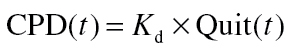 |
(3) |
Highlighted by the lack of derivative and time constant terms, Equation 3 indicates that quit-induced changes in CPD are immediate. K d, the gain for the Quit Attempt Process, quantifies the net change in CPD resulting from the quit attempt. As Quit is a step from 0 to 1 on the target quit date, Equation 3 indicates that on the quit day, CPD decreases by 15.01 and 10.24 cigarettes for AC and PNc groups, respectively (see K d values in Table 2).
Craving Self-Regulator
The ODE that adequately represents the Craving Self- Regulator is:
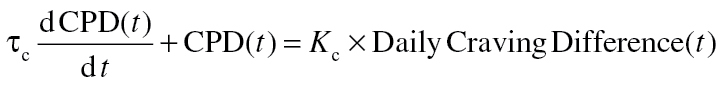 |
(4) |
K c quantifies the change in CPD resulting from changes in Daily Craving Difference (=Baseline Craving Level − Current Craving): a one point increase in Daily Craving Difference leads to 0.08 and 0.30 cigarette increases in CPD for the AC and PNc groups, respectively. Conversely, a one point decrease in Daily Craving Difference leads to 0.08 and 0.30 cigarette reductions in CPD for the AC and PNc groups, respectively. The time constant τc quantifies the speed at which CPD changes in response to changes in Daily Craving Difference. By definition, 63% of the response in CPD to a change in Daily Craving Difference is achieved in 4.59 days for the AC group but is achieved in only 1.89 days for the PNc group.
These models indicate that the Craving Self-Regulator is the process that models the small and slow resumption of smoking that occurs in both groups after the large initial reduction in CPD (see Figure 3). The AC group’s smaller K c and τc estimates indicate that changes in Daily Craving Difference have a smaller and slower effect on postquit CPD resumption. This may suggest that the treatment diminishes the regulatory (feedback) nature of the overall cessation process.
Craving Generation Process
The Craving Generation Process required the most complex ODE compared to the Quit Attempt Process and Craving Self-Regulator. The differential equation structure that adequately represents the Craving Generation Process is:
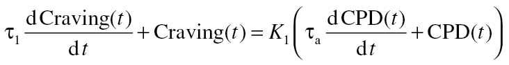 |
(5) |
K 1 quantifies the change in Current Craving per unit change in CPD. As indicated by the K 1 values in Table 2, a one cigarette increase in total daily smoking leads to a net 0.77 point increase in Current Craving for the AC group. Conversely, a one cigarette decrease in CPD leads to a 0.77 point decrease in Current Craving for this group. The time constant τ1 quantifies the speed at which the 0.77 point change in Current Craving occurs per one cigarette change in CPD. The system zero parameter τa is negative for both groups. The negative value indicates a dynamic feature in Current Craving called inverse response, in which Current Craving increases upon quitting before ultimately settling to a value below prequit levels. This inverse response is evident in Figure 3 as well, and it appears that the inverse response is more pronounced in the PNc group than in the AC group.
As seen in Table 2, the standard error bounds are nonoverlapping between the groups for all parameters except for K 1 and τ1. Even with the overlapping standard error bounds for these two parameters, it can still be said that the active treatment appears to facilitate a larger total quit-induced Current Craving decrease relative to the placebo group. This observation is based on Figure 3, which shows that the overall response and confidence intervals for Current Craving predicted by the estimated group models do not overlap as time goes on.
DISCUSSION
The models presented illustrate how dynamic modeling and system identification methods can be used to understand self-regulation within the smoking cessation process. In this regulatory system, Current Craving is the primary output and changes in Current Craving and CPD are fundamentally interrelated. The dynamic models are estimated differential equations that predict day-to-day changes in Current Craving and CPD and reflect the dynamic features observed in clinical trial data for two treatment groups. Notably, the models capture inverse response in Current Craving (quit-induced increase before settling to below prequit levels), a dramatic quit-day drop in CPD, and the slow and small postquit resumption of smoking. These dynamic features are represented by ODE functions that describe the Craving Generation Process, Craving Self-Regulator, and Quit Attempt Process individually and quantify the net change in Current Craving resulting from a one cigarette per day change in CPD (K 1), the characteristics of smoking resumption over time on a group level (K c, τc), and more. Comparing the dynamics predicted by the models (see Figure 3), it appears that the bupropion and counseling combination facilitates more favorable outcomes in the month following initial quit, on a group level.
One interesting aspect of Current Craving is the inverse response apparent in both treatment groups. Consequently, the mathematical expressions representing the Craving Generation Process require a system zero term. It is known (Ogunnaike & Ray, 1994) that dynamical systems with a zero term can represent a sum of two subprocesses in parallel. Here, it can be deduced that one subprocess has a negative gain and fast speed of response, which corresponds to the initial increase in Current Craving that results from the quit-induced decrease in CPD; the second subprocess has a positive gain and a comparatively slower speed of response, which corresponds to gradual reduction of Current Craving over time. This idea of competing subprocesses in the Craving Generation Process is consistent with the understanding that there are opposing immediate and delayed gratification motives during cessation (Bickel et al., 2007).
Potential Directions for Dynamic Modeling
The ability of dynamic modeling to describe observed cessation dynamics, and the fact that the techniques to estimate ODE models and existing software packages to do so are intentionally flexible, suggests that this method may offer a platform to investigate additional aspects of the cessation process. For example, Chandra et al. (2011) used progressive lagged analyses to examine within-day temporal relationships. They identified reciprocal relationships in which high craving levels in a 2-hr time period led to high smoking rates in subsequent 2-hr blocks, and high smoking rates in a 2-hr block led to lower craving levels in later blocks. The models presented here were able to describe dynamics of the cessation in the important first month of a quit attempt and therefore did not require within-day data. However, the distinct and separate questions addressed Chandra et al. (2011) could be examined with dynamic models. More specifically, with ILD consisting of more intensive measurements and simple adjustments to the described dynamic modeling procedure, models of within-day self-regulation can be estimated. As the self-regulation system presented can parsimoniously represent the Current Craving–CPD interrelationship, dynamic models of within-day changes in craving levels and smoking rates may provide a unified model of both reciprocal relationships identified in Chandra et al. (2011). Dynamic models could also be used to describe multimonth or multiyear cessation dynamics, even though the assumption of constant parameter values in Table 2 would likely not hold over significantly longer timeframes. Straightforward system identification techniques exist that could estimate models in which a given set of estimates are assumed to be time invariant only over a bounded time interval (Novara, Lopes dos Santos, Azevedo Perdicoulis, Ramos, & Rivera, 2011). Such models could account for the hypothesis that a long-term smoking cessation process involves separate, discrete steps (DiClemente et al., 1991).
The current research could also be extended to address issues of environmental impact. The ILD used here was collected via EMA protocols and so the resulting models provide a more comprehensive description of the CPD and Craving dynamics in that the models estimated are produced using data collected in real-world (nonlaboratory) settings while subject to pressures of real-life experiences (McCarthy et al., 2008a; Shiffman et al., 2008). However, the role of the environment and/or smoking cues on this self-regulatory process could be more explicitly investigated with this engineering approach. To do so, the ODEs shown would be modified in a straightforward manner and used in combination with additional EMA data. The models would be augmented to explicitly account for the effect of contextual factors (e.g., hypothesized smoking cues), which would be included as exogenous variables, like the Quit variable in Figure 1. Models that explicitly account for a relevant contextual variable would be expected to explain more variability in the data; notably, these models would have higher goodness-of-fit values compared to those of models that do not explicitly consider the contextual variable. The resulting expressions would also characterize a contextual variable’s effect on smoking self-regulation through parameter estimates (e.g., gains and time constants). Altogether, this methodology may offer a framework to better leverage ILD collected via EMA, facilitating identification of influential environmental factors and smoking cues.
In addition to illustrating the value of the engineering approach employed, the accuracy of the group average models suggests the three-component self-regulation system depicted in Figure 1 may be an appropriate starting point for future modeling efforts. For instance, dynamic models of self-regulation in individual abstainers may be of interest. Using identical estimation methods and equation structures as those presented here, Timms et al. (2012, 2013) give examples of such idiographic dynamic models for two subjects from the UW-CTRI clinical trial. These idiographic models are the same equation structures as Equations 3–5, but the parameter values estimated from the single subject ILD reflect the dynamic nature of each individual’s Craving Generation Process, Craving Self-Regulator, and Quit Attempt Process. For example, the estimated value of the Craving Self-Regulator’s gain (K c) is near-zero for an individual that effectively had no postquit CPD resumption. Conversely, the gain estimate is significantly larger for an individual that had full postquit smoking resumption (Timms et al., 2012, 2013).
Although this article focuses on the Current Craving–CPD relationship specifically, future work could draw from the dynamic modeling approach to examine additional factors of interest that may act as sources of interindividual variability, such as self-efficacy, physiological conditions, and socioeconomic status. Identification of reliable idiographic dynamic models poses challenges as model reliability ultimately depends on the quality of data used in parameter estimation, and collection of single subject data may not include explicit measurement of all sources of variability. However, the modeling challenge associated with noisy single subject data could be mitigated through novel clinical trial designs that draw from optimal experimental design in system identification (Deshpande, Rivera, & Younger, 2012; Ljung, 1999; Rivera, Lee, Mittelmann, & Braun, 2009). Such a clinical trial would seek to manipulate an exogenous variable over time (e.g., counseling frequency) resulting in ILD (e.g., Current Craving). These study design strategies can support collection of ILD with greater signal-to-noise ratios and less correlation between variables (Ljung, 1999). The data collected from such a clinical trial may be more informative in that it captures a more rigorous picture of the dynamic nature in a system, as opposed to a system’s dynamic response to one type of input change in one variable (Deshpande et al., 2012; Ljung, 1999).
Implications for Interventions
Dynamic models of self-regulated smoking cessation behavior change may also help inform intervention development. Generally, the Current Craving–CPD interrelationship evident here suggests that an intervention that targets either Current Craving or CPD will affect both quantities. Furthermore, the models suggest the Quit Attempt Process is responsible for the initial decrease in CPD immediately following a quit attempt, while the Craving Self-Regulator is responsible for postquit resumption. Although these processes both affect CPD, they do so independently of one another and therefore offer two distinct targets for interventions. Future clinical trials may want to identify intervention strategies that explicitly target these separate cessation processes (Timms et al., 2013).
Use of the models presented in simulation studies could also help advance treatment development. In this article, simulation is used to evaluate how well estimated ODEs describe the Current Craving and CPD ILD. Engineers routinely use simulations to investigate how a system could be augmented to obtain more favorable outputs. In behavioral science settings, candidate mechanisms of effective interventions could be explored through simulation using dynamic self-regulation models. Timms et al. (2013) developed a model of smoking cessation behavior change for a hypothetical patient. These mathematical expressions describe the system in Figure 1 and employ the same equation structures found in Equations 3–5. However, the parameters for these ODEs were chosen to represent a hypothetical difficult patient who is predisposed to cessation failure—that is, the parameters reflect increases in Current Craving corresponding to an initial decrease in CPD, followed by a settling of Current Craving back to prequit levels as the patient fully resumes smoking. These ODEs reflect a “worst-case scenario” for cessation. Through simulation, two new mathematical functions are found that affect Current Craving and Daily Craving Difference in a manner that promotes successful cessation in the hypothetical patient (Timms et al., 2013).
Finally, a significant advantage of dynamic self-regulation models is their potential connection to time-varying, personalized, adaptive smoking cessation interventions. Dynamic models can be used in conjunction with control engineering principles to design intervention algorithms that define how treatment components should be adjusted (e.g., increased counseling frequency) based on tailoring variable measurements (e.g., current withdrawal symptoms). Such an approach is appealing given control engineering’s emphasis on systematic optimization, meaning algorithms could be designed to specify intervention dosage adjustments that support fast quit success within practical constraints (e.g., medication dose toxicity and resource management issues). Moreover, the algorithmic nature of the dynamical systems approach supports rapid treatment adaptation, as would be required by effective ecological momentary interventions that optimally leverage mobile technologies and control engineering principles (Deshpande et al., 2011; Dong et al., 2013; Nandola & Rivera, 2013; Rivera et al., 2007). In summary, this article introduces an engineering approach to analysis of ILD that describes self-regulation in the smoking cessation process more comprehensively than existing analytic approaches.
SUPPLEMENTARY MATERIAL
Supplementary Material can be found online at http://www.ntr.oxfordjournals.org.
FUNDING
This work was supported by an award from the American Heart Association , the Office of Behavioral and Social Sciences Research, and the National Institute on Drug Abuse at the National Institutes of Health (K25 DA021173, R21 DA024266, P50 DA10075, and F31 DA035035).
DECLARATION OF INTERESTS
None declared.
ACKNOWLEDGMENT
The content is solely the responsibility of the authors and does not necessarily represent the views of the National Institutes of Health.
REFERENCES
- Bhadra A., Ionides E. L., Laneri K., Pascual M., Bouma M., Dhiman R. C. (2011). Malaria in northwest India: Data analysis via partially observed stochastic differential equation models driven by Lévy Noise. Journal of the American Statistical Association, 106, 440–451. 10.1198/jasa.2011.ap10323 [Google Scholar]
- Bickel W., Miller M., Yi R., Kowal B., Lindquist D., Pitcock J. (2007). Behavioral and neuroeconomics of drug addiction: Competing neural systems and temporal discounting processes. Drug and Alcohol Dependence, 90, S85–S91. 10.1016/j.drugalcdep.2006.09.016 [DOI] [PMC free article] [PubMed] [Google Scholar]
- Boker S. M. (2012). Dynamical systems and differential equation models of change. In Cooper H., Panter A., Camic P., Gonzalez R., Long D., Sher K. (Eds.), APA Handbook of Research Methods in Psychology (Vol. 3, pp. 323–333). Washington, DC: American Psychological Association [Google Scholar]
- Boker S. M., Nesselroade J. (2002). A method for modeling the intrinsic dynamics of intraindividual variability: Recovering the parameters of simulated oscillators in multi-wave panel data. Multivariate Behavioral Research, 37, 127–160. 10.1207/S15327906MBR3701_06 [DOI] [PubMed] [Google Scholar]
- Bolt D. M., Piper M. E., Theobald W. E., Baker T. B. (2012). Why two smoking cessation agents work better than one: Role of craving suppression. Journal of Consulting and Clinical Psychology, 80, 54–65. 10.1037/a0026366 [DOI] [PMC free article] [PubMed] [Google Scholar]
- Carver C., Scheier M. (1998). On the Self-Regulation of Behavior. New York, NY: Cambridge University Press [Google Scholar]
- Chandra S., Scharf D., Shiffman S. (2011). Within-day temporal patterns of smoking, withdrawal symptoms, and craving. Drug and Alcohol Dependence, 117, 118–125. 10.1016/j.drugalcdep.2010.12.027 [DOI] [PMC free article] [PubMed] [Google Scholar]
- Deshpande S., Nandola N. N., Rivera D. E., Younger J. (2011). A control engineering approach for designing an optimized treatment plan for fibromyalgia. Proceedings of the 2011 American Control Conference, San Francisco, CA (pp. 4798–4803). [DOI] [PMC free article] [PubMed] [Google Scholar]
- Deshpande S., Rivera D. E., Younger J. (2012). Towards patient-friendly input signal design for optimized pain treatment interventions. Proceedings of the 16th IFAC Symposium on System Identification, Brussels, Belgium (pp. 1311–1316). 10.3182/20120711-3-BE-2027.00413 [Google Scholar]
- DiClemente C. C., Prochaska J. O., Fairhurst S. K., Velicer W. F., Velasquez M. M., Rossi J. S. (1991). The process of smoking cessation: An analysis of precontemplation, contemplation, and preparation stages of change. Journal of Consulting and Clinical Psychology, 59, 295–304 [DOI] [PubMed] [Google Scholar]
- Dong Y., Rivera D. E., Downs D., Savage J., Thomas D., Collins L. M. (2013). Hybrid model predictive control for optimizing gestational weight gain behavioral interventions. Proceedings of the 2013 American Control Conference, Washington, DC (pp. 1970–1975). [DOI] [PMC free article] [PubMed] [Google Scholar]
- Fiore M. C., Jaen C. R., Baker T. B., Bailey W. B., Benowitz N. L., Curry S. J, … Wewers M. E. (2008). Treating Tobacco Use and Dependence: 2008 Update. Clinical Practice Guideline. Rockville, MD: U.S. Department of Health and Human Services; Retrieved from http://bphc.hrsa.gov/buckets/treatingtobacco.pdf [Google Scholar]
- Galea S., Hall C., Kaplan G. A. (2009). Social epidemiology and complex system dynamic modelling as applied to health behaviour and drug use research. The International Journal on Drug Policy, 20, 209–216. 10.1016/j.drugpo.2008.08.005 [DOI] [PMC free article] [PubMed] [Google Scholar]
- Ionides E. L., Bretó C., King A. A. (2006). Inference for nonlinear dynamical systems. Proceedings of the National Academy of Sciences of the United States of America, 103, 18438–18443 [DOI] [PMC free article] [PubMed] [Google Scholar]
- Ljung L. (1999). System Identification: Theory for the User (2nd ed.). Englewood Cliffs, NJ: Prentice-Hall, Inc [Google Scholar]
- Ljung L. (2003). System Identification Toolbox for Use With MATLAB: User’s Guide. Natick, MA: The MathWorks, Inc [Google Scholar]
- Ljung L. (2012). Version 8 of the MATLAB system identification toolbox. Proceedings of the 16th IFAC Symposium on System Identification, Brussels, Belgium (pp. 1826–1831). 10.3182/20120711-3-BE-2027.00061 [Google Scholar]
- MathWorks. (2013). pem: Prediction error estimate for linear or nonlinear model Retrieved April 1, 2013, from http://www.mathworks.com/help/ident/ref/pem.html
- McCarthy D. E., Piasecki T. M., Lawrence D. L., Jorenby D. E., Shiffman S., Baker T. B. (2008b). Psychological mediators of bupropion sustained-release treatment for smoking cessation. Addiction, 103, 1521–1533. 10.1111/ j.1360-0443.2008.02275.x [DOI] [PMC free article] [PubMed] [Google Scholar]
- McCarthy D. E., Piasecki T. M., Lawrence D. L., Jorenby D. E., Shiffman S., Fiore M. C., Baker T. B. (2008a). A randomized controlled clinical trial of bupropion SR and individual smoking cessation counseling. Nicotine & Tobacco Research, 10, 717–729. 10.1080/14622200801968343 [DOI] [PubMed] [Google Scholar]
- Nandola N., Rivera D. E. (2013). An improved formulation of hybrid predictive control with application to production-inventory systems. IEEE Transactions on Control Systems Technology, 21, 121–135. 10.1109/TCST.2011.2177525 [DOI] [PMC free article] [PubMed] [Google Scholar]
- Novara C., Lopes dos Santos P., Azevedo Perdicoulis T. P., Ramos J. A., Rivera D. E. (2011). Introduction. In Lopes dos Santos P., Azevedo Perdicoulis T. P., Novara C., Ramos J. A., Rivera D. E. (Eds.), Linear Parameter-Varying System Identification: New Developments and Trends. Hackensack, NJ: World Scientific Publishing Co., Inc [Google Scholar]
- Ogunnaike B., Ray W. (1994). Process Dynamics, Modeling, and Control. New York, NY: Oxford University Press [Google Scholar]
- Piper M. E., Federman E. B., McCarthy D. E., Bolt D. M., Smith S. S., Fiore M. C., Baker T. B. (2008). Using mediational models to explore the nature of tobacco motivation and tobacco treatment effects. Journal of Abnormal Psychology, 117, 94–105. 10.1037/0021-843X.117.1.94 [DOI] [PubMed] [Google Scholar]
- Riley W. T., Rivera D. E., Atienza A. A., Nilsen W., Allison S. M., Mermelstein R. (2011). Health behavior models in the age of mobile interventions: Are our theories up to the task? Translational Behavioral Medicine, 1, 53–71. 10.1007/s13142-011-0021-7 [DOI] [PMC free article] [PubMed] [Google Scholar]
- Rivera D. E. (2012). Optimized behavioral interventions: What does system identification and control systems engineering have to offer? Proceedings of the 16th IFAC Symposium on System Identification, Brussels, Belgium (pp. 882–893). 10.3182/20120711-3-BE-2027.00427 [Google Scholar]
- Rivera D. E., Lee H., Mittelmann H. D., Braun M. W. (2009). Constrained multisine input signals for plant-friendly identification of chemical process systems. Journal of Process Control, 19, 623–635. 10.1016/j.jprocont.2008.08.006 [Google Scholar]
- Rivera D. E., Pew M., Collins L. (2007). Using engineering control principles to inform the design of adaptive interventions: A conceptual introduction. Drug and Alcohol Dependence, 88, S31–S40. 10.1016/j.drugalcdep.2006.10.020 [DOI] [PMC free article] [PubMed] [Google Scholar]
- Samanta G. P. (2011). Dynamic behaviour for a nonautonomous heroin epidemic model with time delay. Journal of Applied Mathematics and Computing, 25, 161–178. 10.1007/s12190-009-0349-z [Google Scholar]
- Shiffman S. (2006). Reflections on smoking relapse research. Drug and Alcohol Review, 25, 15–20. 10.1080/ 0959230500459479 [DOI] [PubMed] [Google Scholar]
- Shiffman S., Stone A., Hufford M. (2008). Ecological momentary assessment. Annual Review of Psychology, 4, 1–32. 10.1146/annurev.clinpsy.3.022806.091415 [DOI] [PubMed] [Google Scholar]
- Shiyko M. P., Lanza S. T., Tan X., Li R., Shiffman S. (2012). Using the time-varying effect model (TVEM) to examine dynamic associations between negative affect and self confidence on smoking urges: Differences between successful quitters and relapsers. Prevention Science, 13, 288–299. 10.1007/s11121-011-0264-z [DOI] [PMC free article] [PubMed] [Google Scholar]
- Solomon R. L. (1977). An opponent-process theory of acquired motivation: The affective dynamics of addiction. In Maser J. D., Seligman M. E. P. (Eds.), Psychopathology: Experimental Models (pp. 66–103). San Francisco, CA: W. H. Freeman [Google Scholar]
- Solomon R. L., Corbit J. D. (1974). An opponent-process theory of motivation. I. Temporal dynamics of affect. Psychological Review, 81, 119–145. 10.1037/h0036128 [DOI] [PubMed] [Google Scholar]
- Tan X., Shiyko M. P., Li R., Li Y., Dierker L. (2012). A time-varying effect model for intensive longitudinal data. Psychological Methods, 17, 61–77. 10.1037/a0025814 [DOI] [PMC free article] [PubMed] [Google Scholar]
- Timms K. P., Rivera D. E., Collins L. M., Piper M. E. (2012). System identification modeling of a smoking cessation intervention. Proceedings of the 16th IFAC Symposium on System Identification, Brussels, Belgium (pp. 786–791). 10.3182/20120711-3-BE-2027.00205 [Google Scholar]
- Timms K. P., Rivera D. E., Collins L. M., Piper M. E. (2013). Control systems engineering for understanding and optimizing smoking cessation interventions. Proceedings of the 2013 American Control Conference, Washington, DC (pp. 1967–1972). [DOI] [PMC free article] [PubMed] [Google Scholar]
- Trail J. B., Collins L. M., Rivera D. E., Li R., Piper M. E., Baker T. B. (in press). Functional data analysis for dynamical system identification of behavioral processes. Psychological Methods. [DOI] [PMC free article] [PubMed] [Google Scholar]
- Velicer W. F., Redding C. A., Richmond R. L., Greeley J., Swift W. (1992). A time series investigation of three nicotine regulation models. Addictive Behaviors, 17, 325–345. 10.1016/0306-4603(92)90039-X [DOI] [PubMed] [Google Scholar]
- Walls T., Schafer J. (2006). Models for Intensive Longitudinal Data. Oxford, UK: Oxford University Press [Google Scholar]
- Watson D., Clark L. A., Tellegen A. (1988). Development and validation of brief measures of positive and negative affect: The PANAS scales. Journal of Personality and Social Psychology, 54, 1063–1070. 10.1037/0022-3514.54.6.1063 [DOI] [PubMed] [Google Scholar]
- Welsch S. K., Smith S. S., Wetter D. W., Jorenby D. E., Fiore M. C., Baker T. B. (1999). Development and validation of the Wisconsin Smoking Withdrawal Scale. Experimental and Clinical Psychopharmacology, 7, 354–361. 10.1037/1064-1297.7.4.354 [DOI] [PubMed] [Google Scholar]