

Abstract
Introduction:
Ecological momentary assessments (EMAs) are useful for understanding both between- and within-subject dynamic changes in smoking and mood. Modeling 2 moods (positive affect [PA] and negative affect [NA], PA and NA) simultaneously will better enable researchers to explore the association between mood variables and what influences them at both the momentary and subject level.
Methods:
The EMA component of a natural history study of adolescent smoking was analyzed with a bivariate location-scale mixed-effects model. The proposed model separately estimates the between- and within-subject variances and jointly models the 2 mood constructs. A total of 461 adolescents completed the baseline EMA wave, which resulted in 14,105 random prompts. Smoking level, represented by the number of smoking events on EMA, entered the model as 2 predictors: one that compared nonsmokers during the EMA week to 1-cigarette smokers, and the second one that estimated the effect of smoking level on mood among smokers.
Results:
Results suggest that nonsmokers had more consistent positive and negative moods compared to 1-cigarette smokers. Among those who smoked, both moods were more consistent at higher smoking levels. The effects of smoking level were greater for NA than for PA. The within-subject association between mood constructs was negative and strongest among 1-cigarette smokers; the within-subject association between positive and negative moods was negatively associated with smoking.
Conclusions:
Mood variation and association between mood constructs varied across smoking levels. The most infrequent smokers were characterized with more inconsistent moods, whereas mood was more consistent for subjects with higher smoking levels.
INTRODUCTION
Modern methods of data collection, such as ecological momentary assessment (EMA), yield relatively large numbers of observations per subject. EMA methods are used to study a wide range of behaviors, experiences, and conditions in the settings in which they naturally occur (Shiffman, Stone, & Hufford, 2008). EMA is useful for understanding both between- and within-subject dynamic changes in smoking and mood (Mermelstein, Hedeker, & Weinstein, 2010).
EMA methods yield data that are clustered within subjects and should be analyzed by methods that take into account the correlated observations. For a single clustered outcome, mixed-effects models are well developed and are a popular method for analyzing longitudinal data (Hedeker & Gibbons, 2006). In practice, however, many studies collect information on multiple outcomes (e.g., smoking level, withdrawal symptoms, and self-efficacy ratings). These outcomes are usually measured concurrently and repeatedly within each subject over time. Multiple outcomes, if modeled jointly, might help in addressing a variety of scientific questions about the relationships among the outcomes. For example, one could examine how craving and self-efficacy for quitting change in tandem. These multiple outcomes induce two types of associations: (a) at the subject level—association between the subject-average levels of outcomes, also called between-subject (BS) covariance and (b) at the momentary level—within-subject association for two outcomes at the measurement level, also called within-subject (WS) covariance. The classic joint mixed model (Verbeke & Davidian, 2009) can be extended to allow correlated error terms in addition to the correlated random effects. Additionally, the covariance of the random effects and the covariance of the error terms can themselves be modeled by separate linear models. This helps to investigate how the associations between the outcomes change for different population subgroups or different treatment conditions. For example, the association between two outcomes may vary by sex, age, racial group, or by exposure to different treatments.
In this article, we propose to simultaneously model two mood states, positive affect (PA) and negative affect (NA), as they relate to smoking in adolescents. Adolescents may be motivated to smoke either to reduce NA, enhance PA, or both (Baker, Brandon, & Chassin, 2004). These different mood effects may represent distinct motivational processes as well as risk for smoking escalation. Thus, considering the joint relationships of NA and PA with smoking addresses both theoretical and practical issues related to adolescent smoking. To date, many analytic approaches have been limited by their consideration of individual mood states singularly or by not disentangling the BS and WS effects. Disentangling the BS effects (i.e., whether different smoking levels are associated with different levels of mood variability across subjects) from WS effects (whether an individual’s variation in mood differs by smoking level) is critical. Also, whereas the majority of research is concerned with mean modeling of outcomes, modeling outcome variation might be of practical importance. In this regard, in a recent paper by Hedeker, Mermelstein, and Demirtas (2012), the BS and WS variances in PA and NA were separately modeled as a log-linear function of covariates. Here, we extend this approach by jointly modeling PA and NA in a much more comprehensive manner.
NA and smoking are strongly linked across both adolescent and adult populations (Kassel, Stroud, & Paronis, 2003). Youth who have higher expectancies for smoking to improve NA are more likely to escalate in smoking (Heinz, Kassel, Berbaum, & Mermelstein, 2010), and those who report using cigarettes primarily to ameliorate NA report greater intentions to continue smoking compared to those who cite other motivations (Stevens, Colwell, Smith, Robinson, & McMillan, 2005). Variability in NA may also be just as important as overall level of NA in predicting future smoking. Previous research using EMA data from both a similar (Weinstein, Mermelstein, Shiffman, & Flay, 2008) and the current sample (Weinstien & Mermelstein, in press) of adolescents revealed that higher levels of negative mood variability differentiated those who escalated in their smoking compared to those who maintained lower or higher levels of cigarette use. These effects remained even when controlling for mean level of NA, emphasizing the necessity to examine both mean level of mood as well as variability when identifying risk for escalation.
PA has received considerably less empirical attention than NA. PA enhancement, however, may reflect a separate motivational state for smoking and may be especially important in adolescents (Baker et al., 2004). Although some researchers promote the bipolarity of PA and NA on one dimension (Russell & Carroll, 1999), others (Watson, Clark, & Tellegen, 1988) stress that PA and NA are orthogonal constructs. One recent review synthesizing data linking smoking to various dimensions of affect concluded that studies examining PA and NA simultaneously document their distinctness (Ameringer & Leventhal, 2010). Joint modeling of the PA and NA association might help in addressing questions about the dimensionality of affect and whether the dimensions of affect (positive and negative) change differentially with the level of smoking.
How smoking among adolescents is conceptualized and handled analytically is yet another critical issue. Much of extant research uses standard definitions of current smoking among adolescents to dichotomize smoking (e.g., considering any past 30-day cigarette use as “smoking”: Johnston, O’Malley, Bachman, & Schulenberg, 2012) or evaluates smoking level as a continuous construct based on cigarettes per day. However, in adolescents, there is value in differentiating between no smoking and low-level smoking to address issues of initiation; and then among those who smoke, differentiating smoking level as a way of addressing escalation beyond initiation. By assessing both stage and continuous smoking behavior in adolescents, we might better elucidate smoking’s link to mood.
The present study builds upon previous work on smoking-related PA and NA change and variability in two primary ways. First, the modeling approach allows for the joint examination of PA and NA outcomes as well as the examination of associations between PA and NA across smoking levels. Second, this approach facilitates the separation of BS and WS effects of smoking on PA and NA. In addition to illustrating a relatively novel analytic approach, this study may help to confirm affect-related motivating factors of cigarette smoking, as well as to build upon the evidence for the dimensionality of affect in this population.
METHODS
Participants
Data for this article come from a longitudinal, natural history of adolescent smoking (“Social-Emotional Contexts of Adolescent Smoking Patterns”). Based on smoking experience (oversampling for smoking in past 90 days), youth (3,654) were invited to participate in the longitudinal study. Youth were enrolled after written parental consent and student assent was obtained. Of those invited, 1,344 agreed to participate (36.8%) and 1,263 (94.0%) completed the baseline wave. Agreement to participate did not vary by smoking history, race/ethnicity, or parental smoking, but girls were slightly more likely to agree to participate than boys.
The sample for the current study included a subset of participants from the overall longitudinal study (N = 1,263) who provided EMA data at baseline (N = 461). Students from 9th and 10th grades were invited into the EMA study if they were former experimenters (n = 112), current experimenters (n = 249), or regular smokers (n = 100); thus, all participants in the current study had smoking experience. Participants ranged in age from 13.85 to 17.29 years (M = 15.67 years, SD = 0.61); 50.7% were 9th graders; 55.1% were girls; and 56.8% White, 15.8% Black, 20% Latino, 2.8% Asian/Pacific Islander, and 4.6% other/biracial.
Procedures
All procedures received approval from the Institutional Review Board at the University of Illinois at Chicago. Data collection modalities included self-report questionnaires on smoking and psychosocial functioning and EMA interviews via handheld computers.
All participants were trained on the EMA device at the beginning of the data week and carried the device for seven consecutive days at each wave. Students completed EMA interviews in response to random prompts (“random prompt” interviews; approximately five times per day) as well as event-recorded smoking events. Analyses here include data only from the random prompts at the baseline wave. Across the 461 participants, 14,105 random prompts were completed (mean of 30 prompts per adolescent, range from 7 to 71).
EMA Measures
Two outcome measures considered in the analysis were a subject’s PA and NA. Youth were asked to rate their mood just prior to the random prompt. Both PA and NA consisted of the average of several mood items, which were identified via factor analysis. PA included the following mood items: happy, relaxed, cheerful, confident, and accepted by others. Higher values of PA indicated relatively better mood. NA included the following items: sad, stressed, angry, frustrated, and irritable. Higher values of NA indicated relatively more negative mood. Participants rated each adjective on a 10-point Likert scale (1 = not at all; 10 = very). Over all responses, PA had a mean of 6.80 (SD = 1.93) and NA mean was 3.46 (SD = 2.25). The empirical correlation between PA and NA was estimated to be negative 0.57 (p < .0001).
The main predictor of interest was smoking level, a subject-level predictor calculated as the ratio of the number of smoking events (during the EMA collection period) over the total number of EMA prompts (“random prompts” interviews + “smoke” interviews). All participants were trained to actively event record every episode when they smoked, which resulted in a number of recorded smoking events per participant. Smoking level was used as a piecewise covariate, meaning that two covariates for smoking effect were used in the model. The first covariate compared nonsmokers to one-cigarette smokers (lowest nonzero smoking level); the second covariate estimated the slope of the smoking level among smokers. A total of 234 participants, 50.8%, had at least one smoking event during the baseline wave. Among adolescents who reported smoking, a total of 58 (24.8%) reported smoking one cigarette (one smoking event) during the EMA week. Among smokers, the average proportion of smoking events over the total number of smoking events and random prompts was 0.13. This corresponds to smoking five cigarettes on average during the week of EMA data collection, range 1–42 cigarettes. Among smokers, the 25th percentile, median, and 75th percentile of smoking proportion (number of cigarettes) were at 0.05 (2 cigarettes), 0.08 (3 cigarettes), and 0.18 (6 cigarettes), respectively. Additional covariates included in the model were gender and school grade.
Data analyses
Consider the following bivariate mixed-effects model for two repeated measurements  and
and  , such as PA and NA, for subject i (i = 1, …, N)
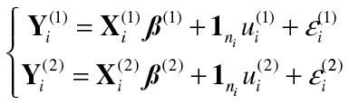 (1) (1)
|
Here  is a
is a 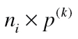 matrix of regressors (i.e., fixed effects),
  is a
is a  —vector of regression coefficients, and
  is a subject’s random effect, k = 1, 2. The random effects
  and
and  indicate the influence of individual i on his/her mean response level. The distribution of these random effects is assumed to be a normal with mean zero and variance–covariance matrix
 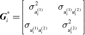 . The errors
  and
and  are assumed to be normally distributed with zero mean and variance–covariance matrix
 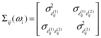 and are independent of the random effects. The nonzero covariances (of random effects)
  and (error terms)
  induce association between the responses. Thus, the overall association between
  and
and  has two components. The first component (BS) comes from the association between subject-level means of the outcome variables, with the covariance
  between the two random effects characterizing this association. If the subject-level means are not correlated, then
  will be estimated to be zero. If the covariance is positive, then average levels of
  and
and  increase/decrease together. Given the association of the mean levels, observations within a subject
  , j = 1, …, n
i, may also be correlated—this is the second component (WS) of the association between the outcomes. When the observations within a subject are correlated, it indicates that the residual errors at a given measurement point j are correlated. The model permits separate estimation of the BS and WS association of the outcome variables. In addition to separately estimating BS and WS components of the outcomes association, the BS and WS covariances are modeled by linear models to explore if these outcome associations vary between subpopulations of subjects.
, j = 1, …, n
i, may also be correlated—this is the second component (WS) of the association between the outcomes. When the observations within a subject are correlated, it indicates that the residual errors at a given measurement point j are correlated. The model permits separate estimation of the BS and WS association of the outcome variables. In addition to separately estimating BS and WS components of the outcomes association, the BS and WS covariances are modeled by linear models to explore if these outcome associations vary between subpopulations of subjects.
 (2) (2)
|
 (3) (3)
|
Here, Equation (2) models the BS covariance as a function of subject-level covariates  and Equation (3) models the WS covariance as a function of time-varying or subject-level covariates
  . The first elements of vectors
  and
and  are 1, and therefore the first elements in the regression coefficient vectors represent the BS and WS covariance for the reference category (i.e., when all covariates equal 0). The additional parameters in Equations (2) and (3) represent effects of the covariates on the BS and WS covariances, respectively. The set of covariates in models (2) and (3) might be different or the same.
To allow for heterogeneous BS and WS variances, the variances  and
and  of the random effects and variances of the error terms are modeled as log-linear models:
 (4) (4)
|
 (5) (5)
|
The log-linear representation ensures that the variances will be positive, which increase or decrease in a multiplicative manner due to the effects of covariates  and
and  , k = 1, 2. This then allows the BS and WS variances, respectively, to differ between subgroups of subjects. The log-linear representation of the WS variance in Equation (5) also includes a random parameter
  (i.e., the random scale parameter). The subject-level random scale represents the part of a subject’s WS variance that is not explained by covariates. Further details on the variance modeling can be found in Pugach (2012).
In this model,  is a random effect that influences the location or mean of the individual’s outcome, and
  is a random effect that influences an individual’s variance or square of the scale. Thus, the model is expanded with both types of random effects. These four random effects (two for each outcome) are allowed to be correlated with each other. For example, the covariance between the random location and random scale effects indicates the degree to which a subject’s mean level and their variance are associated (e.g., subjects with better average mood are also more consistent in their mood).
The model can be implemented in PROC NLMIXED, SAS Institute, v.9.2, and therefore broadens the potential application of this approach. Sample syntax is available in the Supplementary Appendix to this article.
RESULTS
Two models were estimated and compared using the bivariate location-scale mixed-effects model. The first used smoking level as a continuous covariate. In the second, two covariates for smoking level were used: the first contrasted adolescents who did not smoke at all during the 7 days (nonsmokers) to those who smoked at least once (one-cigarette smokers); the second covariate examined effect of smoking level among those who smoked. This allows relaxing the assumption of a linear association between smoking level and mood. Specifically, two independent variables that represent the effect of smoking estimate (a) the mood difference between nonsmokers and one-cigarette smokers (one vs. none; one-cigarette smoker in Table 1) and (b) how mood varied with smoking level among smokers only (amount smoked in Table 1).
Table 1.
Bivariate Location-Scale Mixed-Effects Model of PA and NA With Piecewise Smoking Predictor (Number of Subjects = 461; Number of Observations = 14,105)
| Submodel | Parameter | Positive affect | Negative affect | ||||
|---|---|---|---|---|---|---|---|
| Estimate | SE | p value | Estimate | SE | p value | ||
| Fixed effect covariates | Intercept | 6.7285 | 0.1160 | <.0001 | 3.5756 | 0.1369 | <.0001 |
| Male | 0.2988 | 0.1113 | .0075 | −0.5863 | 0.1351 | <.0001 | |
| 10th grade | 0.0128 | 0.1131 | .9098 | 0.0572 | 0.1348 | .6716 | |
| One-cigarette smoker | −0.2329 | 0.1364 | .0885 | 0.4709 | 0.1671 | .0050 | |
| Amount smoked | 0.4369 | 0.6760 | .5184 | −1.6370 | 0.7663 | .0332 | |
| WS variance | Intercept | 0.8557 | 0.0488 | <.0001 | 0.9606 | 0.0596 | <.0001 |
| Male | −0.2472 | 0.0491 | <.0001 | −0.4181 | 0.0599 | <.0001 | |
| 10th grade | −0.1436 | 0.0485 | .0033 | −0.0918 | 0.0594 | .1226 | |
| One-cigarette smoker | 0.1154 | 0.0588 | .0504 | 0.3533 | 0.0721 | <.0001 | |
| Amount smoked | −0.5968 | 0.2953 | .0439 | −1.3948 | 0.3592 | .0001 | |
| BS variance | Intercept | 0.2600 | 0.0905 | .0042 | 0.6542 | 0.0863 | <.0001 |
| Male | −0.1729 | 0.1201 | .1507 | −0.3685 | 0.1169 | .0017 | |
| 10th grade | −0.1786 | 0.1155 | .1227 | 0.1883 | 0.1114 | .0915 | |
| One-cigarette smoker | 0.1090 | 0.1454 | .4538 | 0.2024 | 0.1360 | .1373 | |
| Amount smoked | −0.1041 | 0.8029 | .8968 | −0.9070 | 0.6097 | .1375 | |
| Random scale variance | −1.6365 | 0.0850 | <.0001 | −1.1194 | 0.0828 | <.0001 | |
| Submodel | Parameter | Estimate | SE | p value | |||
| WS covariance | Intercept | −1.4173 | 0.0490 | <.0001 | |||
| Male | 0.6067 | 0.0438 | <.0001 | ||||
| 10th grade | 0.2102 | 0.0425 | <.0001 | ||||
| One-cigarette smoker | −0.2627 | 0.0530 | <.0001 | ||||
| Amount smoked | 1.8999 | 0.2060 | <.0001 | ||||
| BS covariance | Intercept | −0.9010 | 0.1145 | <.0001 | |||
| Male | 0.2925 | 0.1564 | .0621 | ||||
| 10th grade | −0.1896 | 0.1455 | .1932 | ||||
| One-cigarette smoker | −0.2494 | 0.1926 | .1961 | ||||
| Amount smoked | 1.2584 | 0.7832 | .1088 | ||||
| Random location (u) and random scale (ω) covariance |
|
0.0303 | 0.0160 | .0586 | |||

|
−0.1752 | 0.0297 | <.0001 | ||||
|
0.0176 | 0.0337 | .6022 | ||||

|
−0.2294 | 0.0355 | <.0001 | ||||
|
0.4006 | 0.0443 | <.0001 | ||||
Note. BS = between-subject; WS = within-subject.
Comparing the model with the piecewise smoking level predictor to the model with the continuous smoking level predictor, the likelihood ratio test statistic was 47 with 8 df. Thus, using piecewise regression significantly improves the model fit to the data, p < .0001.
Results of the piecewise regression model are presented in Table 1 and suggest that nonsmokers had lower NA compared to one-cigarette smokers. Among smokers, higher smoking level was associated with lower NA. The pattern was similar for PA (better average mood for nonsmokers and high level smokers), but the effects were not significant. Males had significantly higher PA and lower NA compared to females.
Figure 1a and b depicts the estimated PA and NA means comparing the two models: model with the piecewise and model with continuous regressors for smoking level. The solid lines represent estimates from the piecewise regression model and the dashed lines represent estimates from the models with continuous smoking level. Smoking level (horizontal axis) ranges from 0 (nonsmokers) to 0.20 (75th percentile of smoking level among smokers). The break-point in the solid line is at 0.014, which is the lowest nonzero amount of smoking in our sample. As one can see from Figure 1a and b, mean values of PA and NA for subjects with the highest smoking level were nearly the same as for nonsmokers.
Figure 1.

Estimated mean positive affect (PA; a) and mean negative affect (NA; b) for different smoking levels. Solid line = piecewise smoking; dashed line = continuous smoking; dotted vertical line = break-point in the slope of smoking effect, occurred at 0.014 smoking proportion (one cigarette).
The WS and BS variance estimates, as well as the estimates of the random scale variances, are presented on the log-scale in Table 1. Exponentiating these estimates provide multiplicative effects of the covariates on the variance(s) in the original metric. Among smokers, higher smoking level was associated with more consistent positive mood ( p = .044). In other words, the WS variability in PA was reduced by a factor of exp(−0.597) = 0.551 with each unit increase in smoking level among smokers. The WS variance modeling of NA showed even stronger results. Among smokers, smoking level was negatively associated with variability in NA; specifically, a higher level of smoking corresponded to more stable NA. WS variability in PA and NA for subjects with the highest number of smoking episodes was comparable in magnitude to WS variability of nonsmokers (see Figure 2a and b, solid lines). The results for NA were much stronger than for PA, both in terms of the mean and WS variance. Males were more consistent than females on both PA and NA, while 10th graders were more consistent on PA than 9th graders.
Figure 2.

Estimated within-subject (WS) positive affect (PA) (a) and negative affect (NA) (b) variance for different smoking levels. Solid line = piecewise smoking; dashed line = continuous smoking; dotted vertical line = break-point in the slope of smoking effect, occurred at 0.014 smoking proportion (one cigarette).
The random scale variances, estimated to be exp(−1.637) = 0.196 for PA and exp(−1.119) = 0.326 for NA, were highly significant. This suggests that significant parts of the variation in the outcomes were due to individual differences (i.e., the covariates did not explain all of a subject’s mood variation).
In terms of BS variance, the only significant effect was seen for males in terms of NA. Thus, males were more homogeneous as a group, compared to females, in terms of negative mood.
The covariance models of the WS and BS association adds another level of understanding of the relationship between the PA and NA mood constructs. The estimated intercept for the WS covariance (association of the responses within a subject at the momentary level) of PA and NA was −1.417 (p < .0001); this is for nonsmoker females in 9th grade. Expressed as a correlation, it equals −0.572. WS correlation is calculated using WS covariance and variances:
 |
For example, for nonsmoker female in 9th grade, the reference category, WS correlation equals
 |
This suggests fairly strong negative association between PA and NA within a subject. The additional covariance model estimates indicate how this association changes between subgroups of subjects. For example, the estimated coefficient for the effect of one-cigarette smokers was −0.263 (p < .0001), suggesting that the WS association between the mood constructs was stronger and more negative for one-cigarette smokers compared to nonsmokers. Among smokers, the WS covariance for smoking level was positive,  (p < .0001); thus, a higher smoking level corresponded to the diminished WS association between PA and NA (see Figure 3). Males and 10th graders exhibited significantly less negative association between the mood constructs.
Figure 3.

Estimated within-subject (WS) covariance between positive affect (PA) and negative affect (NA) for different smoking levels. Solid line = piecewise smoking; dashed line = continuous smoking; dotted vertical line = break-point in the slope of smoking effect, occurred at 0.014 smoking proportion (one cigarette).
Although the BS covariance effects of smoking were similar to their WS covariance counterparts, they were not significant. This might be due to the increased power for detecting WS effects (which is based on the momentary data within subjects) than BS effects (which is based on the number of subjects).
The random location and scale parameters were specified as correlated in the model. The estimated covariances of the random location and scale parameters appear at the bottom of Table 1. The covariance of the random location and scale effects for PA was negative indicating that subjects with higher values of PA also had less variable PA mood. This might be an indication of a more trait-like, less situational, quality of PA. On the other hand, it might be a ceiling effect of measurement. Conversely, for NA, the covariance was positive suggesting that subjects with more negative mood (higher NA value) also had more variable NA mood. Alternatively, the positive covariance might reflect a floor effect of measurement. Finally, the PA location and NA scale effects were significantly negatively associated, indicating that subjects with high PA were also very consistent on NA.
DISCUSSION
The bivariate location-scale mixed-effects model was used to assess jointly positive and negative moods as a function of smoking level in adolescents. This approach also facilitated the separation of BS and WS effects of smoking on PA and NA. The results illustrated the utility of a piecewise approach for modeling smoking to capture both a categorical and continuous phenomenon. The approach of modeling two outcomes simultaneously can be easily translated to other theoretical questions such as joint associations between self-efficacy, craving, and smoking reduction. Our results can also be incorporated into both observational and intervention-focused research targeting smoking and mood in adolescent samples.
Results revealed that adolescent one-cigarette smokers exhibited higher NA compared to both nonsmokers and higher level smokers. The results for mean NA diverged from a dose–response relationship often observed in studies examining the mood and smoking association (e.g., Kassel et al., 2003; Windle & Windle, 2001). Nonetheless, findings corroborate a recent longitudinal study showing a dampening effect of depressive symptoms (one component of NA) with smoking progression in adolescents (Audrain-McGovern, Rodriguez, & Kassel, 2009). Developing a consensus regarding affective links to smoking intensity might be especially challenging in adolescents who are smoking at particularly light levels and often exhibit heterogeneous pathways of progression (e.g., Audrain-McGovern et al., 2004). However, by taking this piecewise approach, we could distinguish important mean NA differences not observed when examining smoking entirely categorically or continuously. In contrast to results found for mean NA, smoking level was not a significant predictor of mean PA. However, findings did show a similar pattern to NA mean values. PA results were consistent with the assertion that reward-seeking and PA enhancement are important motivational influences in smoking.
The results also suggested that smoking was associated with both PA and NA momentary variances as well as their momentary covariance. The curvilinear association in PA and NA WS variances suggested that one-cigarette smokers were also most erratic in their momentary mood responses, but mood was more consistent with higher smoking levels. PA variability is thought to be characteristic of normative emotional development in adolescence (Larson, Csikszentmihalyi, & Graef, 1980). Thus, the present study promotes the notion that affects dysregulation, regardless of the context of the variability, may be an important motivating factor involved in smoking progression in adolescents. It is possible that our one-cigarette smoking youth continue to smoke beyond initiation in an attempt to regulate affective instability but are not smoking with enough frequency to achieve longer lasting “medicating” benefits. Furthermore, Weinstein et al. (2008) also found that greater NA variability differentiated those who escalated in their smoking over time, rendering this an important marker for escalation. Given that the one-cigarette smokers exhibited this critical risk factor, results emphasize the necessity of continued use of this modeling approach to better understand an important juncture of adolescent smoking.
The nonlinear association in WS covariance, which reflects strength of association between mood constructs at the momentary level, suggested that PA and NA had the strongest association for one-cigarette smokers, whereas nonsmokers and heavier smokers had less correlated mood responses. This highlights the utility of jointly examining NA and PA and adds support to the multidimensionality of affects. Accordingly, our findings emphasize the need to evaluate both PA and NA among adolescent smokers across levels of smoking. The diminished association in the WS covariance for nonsmokers and heavier smokers might be partly explained by smaller variability in the both mood measures; although the WS variations in both PA and NA for heavier smokers were comparable to nonsmokers, the WS covariance was much smaller for heavier smokers compared to nonsmokers. This suggests that the change in the two-dimensional WS outcomes association cannot be completely explained by a change in unidimensional WS variances.
This study has many strengths, including the use of sophisticated “real-time” methodology to capture daily mood and smoking as well as the innovative statistical modeling approach. However, limitations should be noted. First, the EMA data may not capture every smoking event, and thus we may be missing out on some smoking episodes. Yet, in-depth interviews with participants following the data collection week indicate that the quantity of missing events is negligible. Second, our study sample was generally at high risk for smoking escalation, having oversampled for ever smoking, and we must be cautious about generalizing our findings to more normative populations. Finally, one-cigarette smoking is admittedly an arbitrary cut point. However, this break-point appears to represent an important juncture in smoking progression and well illustrates the capability of this methodological advance.
Modern data collection procedures, such as EMA, provide a fair amount of both WS and BS data and so give rise to the opportunity for modeling of WS and BS variances and covariances as a function of covariates. However, computational difficulties can arise in application of the proposed model for a variety of reasons (e.g., the resulting variance–covariance matrix is not positive definite) leading to nonconvergence of the solution. In such cases, a simpler model is usually warranted (i.e., some model parameters are set to zero and not estimated).
SUPPLEMENTARY MATERIAL
Supplementary Appendix can be found online at http://www.ntr.oxfordjournals.org.
FUNDING
This work was supported by a grant from the National Cancer Institute (P01CA098262).
DECLARATION OF INTERESTS
None declared.
ACKNOWLEDGMENT
The authors thank Siu Chi Wong for assisting with data preparation and management.
REFERENCES
- Ameringer K. J., Leventhal A. M. (2010). Applying the tripartite model of anxiety and depression to cigarette smoking: An integrative review. Nicotine & Tobacco Research, 12, 1183–1194. 10.1093/ntr/ntq174 [DOI] [PMC free article] [PubMed] [Google Scholar]
- Audrain-McGovern J., Rodriguez D., Kassel J. D. (2009). Adolescent smoking and depression: Evidence for self-medication and peer smoking mediation. Addiction, 104, 1743–1756. 10.1111/j.1360-0443.2009.02617.x [DOI] [PMC free article] [PubMed] [Google Scholar]
- Audrain-McGovern J., Rodriguez D., Tercyak K. P., Cuevas J., Rodgers K., Patterson F. (2004). Identifying and characterizing adolescent smoking trajectories. Cancer Epidemiology, Biomarkers & Prevention, 13, 2023–2034 [PubMed] [Google Scholar]
- Baker T. B., Brandon T. H., Chassin L. (2004). Motivational influences on cigarette smoking. Annual Review of Psychology, 55, 463–491. 10.1146/annurev.psych.55.090902.142054 [DOI] [PubMed] [Google Scholar]
- Hedeker D., Gibbons R. D. (2006). Longitudinal data analysis. Hoboken, NJ: John Wiley & Sons [Google Scholar]
- Hedeker D., Mermelstein R. J., Demirtas H. (2012). Modeling between-subject and within-subject variances in ecological momentary assessment data using mixed-effects location scale models. Statistics in Medicine, 31, 3328–3336. 10.1002/sim.5338 [DOI] [PMC free article] [PubMed] [Google Scholar]
- Heinz A. J., Kassel J. D., Berbaum M., Mermelstein R. (2010). Adolescents’ expectancies for smoking to regulate affect predict smoking behavior and nicotine dependence over time. Drug and Alcohol Dependence, 111, 128–135. 10.1016/j.drugalcdep.2010.04.001 [DOI] [PMC free article] [PubMed] [Google Scholar]
- Johnston L. D., O’Malley P. M., Bachman J. G., Schulenberg J. E. (2012). Monitoring the future national survey results on drug use, 1975–2011. Volume I: Secondary school students (760 pp.). Ann Arbor, MI: Institute for Social Research, The University of Michigan [Google Scholar]
- Kassel J. D., Stroud L. R., Paronis C. A. (2003). Smoking, stress, and negative affect: Correlation, causation, and context across stages of smoking. Psychological Bulletin, 129, 270–304. 10.1037/0033-2909.129.2.270 [DOI] [PubMed] [Google Scholar]
- Larson R., Csikszentmihalyi M., Graef R. (1980). Mood variability and the psychosocial adjustment of adolescents. Journal of Youth and Adolescence, 9, 469–490. 10.1007/BF02089885 [DOI] [PubMed] [Google Scholar]
- Mermelstein R., Hedeker D., Weinstein S. (2010). Ecological momentary assessment of mood-smoking relationships in adolescent smokers. In Kassel J. D. (Ed.), Substance abuse and emotion (pp. 217–236). Washington, DC: American Psychological Association [Google Scholar]
- Pugach O. (2012). A bivariate location-scale mixed-effects model (PhD thesis, University of Illinois at Chicago; ). Retrieved from http://search.proquest.com/docview/1284417313/abstract/13D3B429A2875BF7247/7?accountid=14552 [DOI] [PMC free article] [PubMed] [Google Scholar]
- Russell J. A., Carroll J. M. (1999). On the bipolarity of positive and negative affect. Psychological Bulletin, 125, 3–30. 10.1037/0033-2909.125.1.3 [DOI] [PubMed] [Google Scholar]
- Shiffman S., Stone A. A., Hufford M. R. (2008). Eco logical momentary assessment. Annual Review of Clinical Psychology, 4, 1–32. 10.1146/annurev.clinpsy.3.022806.091415 [DOI] [PubMed] [Google Scholar]
- Stevens S. L., Colwell B., Smith D. W., Robinson J., McMillan C. (2005). An exploration of self-reported negative affect by adolescents as a reason for smoking: Implications for tobacco prevention and intervention programs. Preventive Medicine, 41, 589–596. 10.1016/j.ypmed.2004.11.028 [DOI] [PubMed] [Google Scholar]
- Verbeke G., Davidian M. (2009). Joint models for longitudinal data: Introduction and overview. In G. Fitzmaurice, M. Davidian, G. Verbeke & G. Molenberghs (Eds.), Longitudinal data analysis (pp. 319–326). Boca Raton, FL: Chapman & Hall/CRC [Google Scholar]
- Watson D., Clark L. A., Tellegen A. (1988). Development and validation of brief measures of positive and negative affect: The PANAS scales. Journal of Personality and Social Psychology, 54, 1063–1070. 10.1037/0022- 3514.54.6.1063 [DOI] [PubMed] [Google Scholar]
- Weinstein S. M., Mermelstein R., Shiffman S., Flay B. (2008). Mood variability and cigarette smoking escalation among adolescents. Psychology of Addictive Behaviors: Journal of the Society of Psychologists in Addictive Behaviors, 22, 504–513. 10.1037/0893-164X.22.4.504 [DOI] [PMC free article] [PubMed] [Google Scholar]
- Weinstien S. M., Mermelstein R. J. (in press). Influences of mood variability, negative moods, and depression on adolescent cigarette smoking. Psychology of Addictive Behaviors. February 25, 2013. [Epub ahead of print.] [DOI] [PMC free article] [PubMed] [Google Scholar]
- Windle M., Windle R. C. (2001). Depressive symptoms and cigarette smoking among middle adolescents: Prospective associations and intrapersonal and interpersonal influences. Journal of Consulting and Clinical Psychology, 69, 215–226. 10.1037/0022-006X.69.2.215 [PubMed] [Google Scholar]