

Abstract
Random spherically constrained (RSC) single particle reconstruction is a method to obtain structures of membrane proteins embedded in lipid vesicles (liposomes). As in all single-particle cryo-EM methods, structure determination is greatly aided by reliable detection of protein “particles” in micrographs. After fitting and subtraction of the membrane density from a micrograph, normalized cross-correlation (NCC) and estimates of the particle signal amplitude are used to detect particles, using as references the projections of a 3D model. At each pixel position, the NCC is computed with only those references that are allowed by the geometric constraint of the particle’s embedding in the spherical vesicle membrane. We describe an efficient algorithm for computing this position-dependent correlation, and demonstrate its application to selection of membrane-protein particles, GluA2 glutamate receptors, which present very different views from different projection directions.
Keywords: cross-correlation, template matching, RSC reconstruction, glutamate receptor, particle picker
1. Introduction
Random Spherically Constrained (RSC) single particle reconstruction (Jiang et al., 2001; Wang and Sigworth, 2010) is a useful approach for studying the structures of membrane proteins in membrane environments. The proteins are reconstituted into spherical lipid vesicles (liposomes), which in turn are frozen in vitreous ice and imaged by electron cryomicroscopy (cryo-EM). As in all single-particle methods, the automatic “picking”, that is selection, of protein particles in micrographs is an important first step in three-dimensional structure determination. The embedding in spherical lipid vesicles presents both disadvantages and advantages. Vesicles are large (~30 nm diameter) but ideally have only one or two protein particles embedded each one, yielding a low overall density of particles in a micrograph. This low density has made the problem of particle selection particularly important, as in our experience a typical 4k × 4k pixel micrograph contains only about 50 particles. This means that many micrographs must be taken and processed to obtain large datasets. Further, the low density of particles means that the relative density of “non-particles” such as frost balls or other contaminants is high. A further disadvantage is that, to avoid distortion of vesicles, the ice layer must be relatively thick, larger than the diameter of the vesicles; thus the high contrast that is observed with very thin ice layers in cryo-EM specimens cannot be exploited.
On the other hand, an advantage arises from the fact that no particles exist in regions between vesicles, and at a given position relative to the center of a vesicle an embedded particle presents a restricted set of views. We sought to design a particle-picking algorithm that efficiently exploits these geometric constraints.
A popular approach to automatic particle picking involves the search of a micrograph using one or more templates (reference images) using the local correlation function (Roseman, 2003; Zhu et al., 2004; Voss et al., 2009) sometimes combined with other criteria for improved detection (Chen and Grigorieff, 2007; Langlois et al., 2011). The local correlation function is also known in the image-processing literature as the normalized cross-correlation (NCC). The program described here computes the NCC, and another selection criterion derived from the NCC, using reference images that are projections of an initial 3D model for the particles to be discovered. Due to the geometric constraint of embedding a protein particle in a spherical vesicle, two of the three Euler angles of orientation of a particle can be determined, within a fourfold ambiguity, from the position of the particle’s projection in the micrograph. Here we adapt an eigenimage-expansion strategy for multiple-template searching (Sigworth, 2004) to exploit these constraints.
As a test case we consider the GluA2 glutamate receptor, a 400 kDa membrane protein. We simulate images using its known X-ray crystal structure (Sobolevsky et al., 2009), and search for particles in cryo-EM images of GluA2 reconstituted into lipid vesicles.
The following notation is used in this paper. An upper-case variable denotes a matrix or an image; a bold-face variable denotes a vector, while lower-case variable denotes a scalar. The squared norm or “power” of an image X having np pixels with values xi is defined as
and C ∘ X denotes operator C operating on X.
2. Methods
2.1. Spherically-constrained projection geometry
We denote the position of a particle on a spherical vesicle by angles α, β, γ (Fig. 1) which, unlike the standard definition of Euler angles for electron microscopy (Heymann et al., 2005) are defined as three successive rotations of the particle rather than rotations of the coordinate system. The projection direction is the −z axis and the projection plane is the (x, y) plane. The definition of the angles is different from the one we used previously(Jiang et al., 2001) and is designed such that a projection image of a particle with α = 0 has the membrane-protein particle oriented along the y-axis, as is customary in the depiction of membrane-protein structures. The two angles α and β can be determined from the geometrical relationship between the particle and the vesicle. Suppose in the projection image the distance from the vesicle center to the particle’s center of mass is r and the particle’s center of mass is at location (x, y); then the two angles can be described by x = rsinα, y = rcosα, r = (rves ± δ)sinβ where rves is the radius of the three-dimensional vesicle (the distance from the vesicle center to the middle of the lipid bilayer membrane) and δ is the radial distance between the particle’s center of mass and the middle of the bilayer. The two possible signs for δ denote two incorporation directions of the membrane-protein particle, inside-out or right-side out.
Fig. 1.

Spherical-constraint projection. The electron beam travels in the −z direction. The position of the particle’s projection image constrains the Euler angles α and β, while p and p′ denote two different embedding positions in the vesicle which correspond to the same center of mass of the projection image. The standard Euler angles ϕ, θ and ψ defined by (Heymann et al., 2005) are related to these according to (ϕ, θ, ψ) = (γ − 90°, β, α + 90°).
A particle may also be embedded in the upper or lower hemisphere of the vesicle. In Fig. 1 we could say that the particle is embedded right-side out and in the upper hemisphere. Rotations about the membrane normal, through the angle γ, represent the final degree of freedom of the particle. Fig. 2 illustrates projections of the GluA2 glutamate receptor, which has C2 symmetry.
Fig. 2.
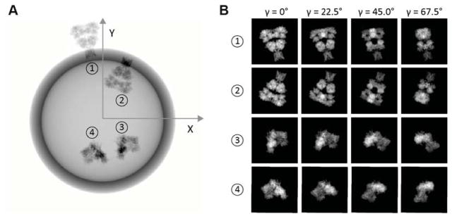
Simulated projections of a membrane protein particle with no CTF applied. Projections were computed from the GluA2 crystal structure, PDB ID: 3KG2. (A) particle at position 1: α = −11°, β = 86°, embedded right-side out on the upper hemisphere; position 2: α = 23°, β = 86°, inside-out on the upper hemisphere; position 3: α = 128°, β = 24°, right-side out on the upper hemisphere; position 4: α = −166°, β = 156°, right-side out on lower hemisphere. The radius of the vesicle is 80 pixels at the scale of 0.3 nm/pixel. (B) projections of particles at 1, 2, 3 and 4 with the same values of α and β but with various γ values, here shown with reversed contrast. The density of the transmembrane region of the particles is shown to be reduced, as is the case after subtraction of membrane density.
2.2. Vesicle membrane subtraction
The RSC method requires that the vesicle-membrane density be subtracted. This is necessary since the vesicles do not all have the same radius, precluding the reconstruction of the entire vesicle with the protein particle. Further, the high density of the vesicle “edge” falls on different parts of the particle image, depending on the particle’s β angle, so it is essential that the density be removed. The processing of a micrograph starts with the determination of the center and radius of each of the perhaps 100 vesicles it contains. With a micrograph downsampled to about 1 nm/pixel, the initial vesicle-finding is done using a simple NCC search with a set of model images of vesicles, typically having radii of 12 to 25 nm with a step size of 1 nm. The step size is chosen to be small compared to the thickness of the vesicle membrane, which is about 5 nm. The position and amplitude of the peaks of the NCC yield an approximate least-squares fit of the vesicle model, which is then refined by a nonlinear least-squares fit of position and radius, one vesicle at a time, to a scalable model (Wang et al., 2006). The end results are the center and radius of each vesicle, determined with ~0.1 nm precision, and an estimate of the contrast in the image of a vesicle. Fig. 2 shows the simulated image of a vesicle, along with images of protein particles as would be obtained after membrane subtraction. It is the membrane-subtracted micrograph which is searched for protein particles.
2.3. Reduced reference set and matched filter
For simplicity let us consider the problem of identifying a single membrane-protein particle in a micrograph that contains one vesicle, after the vesicle-membrane density has been subtracted from the image. This image X can be modeled from the scaled, noiseless particle image Sj:
| (1) |
where a is the image amplitude, x0 is the centered position, and N is independent, zero-mean Gaussian noise.
The underlying particle image Sj, is obtained as:
| (2) |
where M is the 3D model density, Pj is operator for projection along the jth projection direction, C is the contrast transfer function (CTF) and W is a pre-whitening filter (Huang and Penczek, 2004; Sigworth, 2004). The application of a pre-whitening filter to an image makes its noise approximately white and therefore better corresponds to the model (1). The use of a pre-whitening filter is not common in cryo-EM image processing, but the common practice of high-pass filtering of cryo-EM images has a similar effect, dampening the excess low-frequency noise that is found in images.
We assume that a set of these underlying images, Sk; k = 1..n constitute the set of references that we will use for searching for a particle. To find a particle we first calculate, at pixel location x, the cross-correlation of the image X with a reference Sk
| (3) |
where the sum is taken over all pixel locations t in the reference image. We will simplify this calculation by making an eigenimage expansion of the references, as in (Sigworth, 2004). Each of the Sk is approximated by a linear combination of m orthonormal eigenimages Ui obtained by singular value decomposition,
| (4) |
where bik are linear combination coefficients.
Fig. 3A illustrates the first 20 eigenimages computed from a set of almost 4000 references. Successive rows of Fig. 3B compare a few of the approximated images S̃k with the true references Sk when the expansion uses m = 20 terms. As shown in Eq. (15) in (Sigworth, 2004), the squared peak-to-noise ratio of the output of a correlation detector is proportional to which rapidly approaches its maximum value as m increases. Fig. 3C shows that the choice m = 20 yields at least 80% of the maximum value for each of the references; we take this value to be sufficient.
Fig. 3.

(A) The first 20 eigenimages computed from the projections in the GluA2 reference set, after application of the CTF and filtering appropriate to the micrograph shown in Figs. 6 and 7. (B) Shown are six reference images S (the first and the third rows) and the corresponding reconstructions S̃ using m = 20 eigenimages (the second and the fourth rows). (C) The range of relative power |S̃k |2/|Sk |2 for all 3856 references enumerated by k, plotted as a function of the number of terms m in the eigenimage expansion. Choosing m = 20 gives a relative power of 80% or more for all of the references. The set of references was obtained by approximately uniformly-spaced projections of the 3D model with angular steps of ≤ 12°, 15°and 22.5° for α, β and γ, respectively.
We can calculate the cross-correlations of the image X with eigenimages Ui:
| (5) |
and with these, for any single pixel position x0, the cross-correlation of image X with a reference Sk can be approximated by
| (6) |
where the bik are the same coefficients as in Eq. (4).
In our particle-picking algorithm we consider each vesicle separately, and search for particles that may be embedded in that vesicle. The geometric constraint of a particle embedded in a spherical vesicle means that, at a given position in the micrograph, we do not need to search with all possible particle orientations, say 4000 of them; instead, we need consider only a small subset, say 32 orientations. The challenge is to efficiently compute the cross-correlation with the appropriate small subsets of orientations.
To impose the geometric constraint of particle embedding, for each pixel position x0 in the neighborhood of the vesicle we choose references S̃k where
| (7) |
that is, for this pixel position x0, there is a set of allowable indices κ which is indexed by l. The indices κl(x0) refer to references with α and β appropriate to that position in the image, but different l values identifying different particle orientations: right-side out or inside-out, upper or lower hemisphere, and various γ values. If there are nγ different γ values to be tested, then there are nl = 4nγ references that are appropriate to a given position in the projection plane. Fig. 4A is an example of the position-dependent lookup table for l = 1 that gives the indices κ1(x0) in the example used here.
Fig. 4.
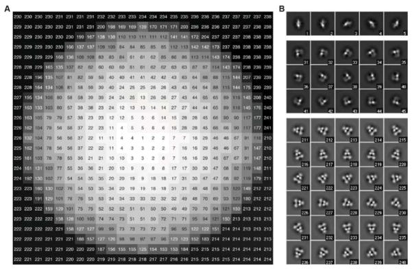
(A) An example of the position-dependent lookup table for κl(x0) for a vesicle of radius 11 pixels having a particle whose center of mass lies 1 pixel outside the membrane center. Values are given for the case l = 1, which corresponds to the particle being right-side out, on the upper hemisphere, and oriented with γ = 0. Each number is the index of the appropriate reference corresponding to that pixel. (B) A few of the references are illustrated. The reference for a “bottom view” of the particle has index 1, while side views of particles have indices of 210 to 241 as the angle α takes on 32 values in a 360 degree range.
The set of position-dependent coefficients can be written as a matrix at each pixel position having the elements
| (8) |
and using this notation the cross-correlation , obtained from Eq. (6) but constrained to the relevant references at each pixel position, is given by
| (9) |
Thus a vector containing the nl values of the cross-correlation with the relevant references, at a given pixel position x0, can be evaluated by the product of a vector Q(x0) and a matrix B(x0). This is the way in which the cross-correlation can be computed against references that vary with pixel position, and is the key for the efficient search for particles under the geometric constraints.
2.4. Normalized cross-correlation
Returning to Eq. (4) for approximating the kth reference image, the orthonormality of the eigenimages Ui implies that the power in a reference image is given by
| (10) |
or, in view of the geometric constraint, we write it as .
The normalized cross-correlation(NCC) of an image with the references can then be computed as
| (11) |
where σX is the standard deviation of the image X in the vicinity of x0. At each position, we find the best index l = λ(x0) by maximizing the NCC:
| (12) |
Thus λ(x0) gives the index of the reference that best matches the image at the position x0. Its determination does not depend on the particular value of σX(x0).
2.5. Signal amplitude as a selection criterion
Many particle-selection algorithms use the values of the NCC to distinguish particles from non-particles in a micrograph. A problem with the NCC is that the local standard deviation σX(x0) of the image must be estimated, but the magnitude of σX depends on the degree of filtering of the image. Thus determining σX requires an arbitrary choice of filtering. We have chosen instead to estimate the value of the scaling amplitude a in the image model (Eq. (1)) to identify valid particles.
An absolute calibration of image contrast is available from the vesicle images. Because the composition of a lipid bilayer membrane is known, a quantitative model of its three-dimensional inner potential V(r) can be computed (Wang et al., 2006), and the weak-phase approximation allows the contrast in the image of a vesicle to be computed as
| (13) |
where Pz is the projection operator, C is the contrast-transfer function, and the amplitude factor aves describes the ratio of image contrast to integrated inner potential. In ideal weak-phase imaging aves = 2σe where the interaction parameter σe is the electron phase shift due to the integral of the inner potential along the electron path; for 200 keV electrons σe = 7.3 mrad/volt·nm (Kirkland, 1998). Fitted values of aves are typically near the theoretical values, but vary by 20–30% over a micrograph.
On the basis of the image contrast aves and a model for a membrane-protein particle, we can predict the value of a for the particle. Specifically, if the 3D model density M in Eq. (2) is expressed in units of the inner potential in volts, then a should be equal to aves. Meanwhile, from the micrograph an estimate of a for a putative particle is obtained as
| (14) |
Because each vesicle image provides a contrast reference, we can search for ã(x0) in the proper range in the vicinity of each vesicle and use its value as a criterion in distinguishing particles from non-particles. The overall scheme for particle picking in the vicinity of one vesicle is diagrammed in Fig. 5.
Fig. 5.

Particle picking process (A) The micrograph is processed by a pre-whitening filter, which is chosen to yield a constant power spectrum of noise in the image. If P(f) is the circularly-averaged power spectrum of particle-free regions of the micrograph, then the filter’s transfer function is chosen to be proportional to P−1/2. (B) Preprocessing of references. From the 3D reference structure a set of 2D projections(~4000 in all) is computed, and each is filtered by the CTF and pre-whitening filter to get the reference set S. Singular value decomposition is then applied to get the eigenimage set U(~20 images). (C) The detection process is diagrammed for the neighborhood of one vesicle. Cross-correlations Qi are calculated between the filtered image and the set of eigenimages by use of FFTs. The subsequent steps are illustrated for a single pixel position x0. Letting κl(x0) index the references relevant to the position x0 on the image of the vesicle, we compute the estimated cross correlation R̃κl with the appropriate references. Maximizing the normalized cross-correlation yields best index l = λ(x0) at each position. The estimated amplitude, computed according to Eq. (14) at this position, is used as a detection criterion.
2.6. Processing of an entire micrograph
The preceding sections have described the search for a particle embedded in a single vesicle. The processing of an entire micrograph starts with the determination of the center, radius and contrast of each of perhaps 100 vesicles. The fitted models of all vesicles of interest are then subtracted from the micrograph, as demonstrated in Fig. 6A–C.
Fig. 6.

Processing of a micrograph. (A) Modeled images of vesicles, obtained by fitting to a micrograph. (B) A portion of the micrograph obtained by merging three exposures, each with a dose of 10 e−/Å2 and with defocus values of 1.9, 5.1 and 17.0 μm. (C) Residual after subtraction of the modeled vesicles from the micrograph. (D) Transfer functions of the circularly-symmetric pre-whitening filter and low-frequency boost filter (top) and overall contrast-transfer functions after application of the filters (bottom). The original CTF (black curve) has three low-frequency peaks due to the contributions from the three defocus levels; information from the second and third exposures was used only up to their first CTF zero. (E) The residual image after application of the pre-whitening filter. (F) The residual image after application of the low-frequency boost filter instead. Shown in each case is a 2k × 2k pixel region of a 4k × 4k micrograph. The width of the region corresponds to 350nm at the specimen. Roughly the upper right quadrant of these images is shown with detected particles in Fig. 7B.
A pre-whitening filter is then constructed for the subtracted micrograph. This is done by computing the average power spectrum for the lowest-variance regions of the micrograph, and the filter transfer function is computed to render the spectrum flat, as demonstrated in Fig. 6D and E. Meanwhile a large set of projections of the 3D search model is computed, and each projection is filtered by the combination of the pre-whitening filter and the CTF. By singular-value decomposition (SVD) the eigenimages are computed (Fig. 5B) along with the coefficients bik as in Eq. (4). For a typical micrograph containing 100 vesicles the application of the CTF and calculation of the SVD takes only a few seconds, less computer time than the 100 cross-correlation searches. Therefore it is not expensive to accommodate images with differing CTFs by simply repeating these computation steps for each image.
At this point the vicinity of each vesicle position is searched in turn. The first step in the search is to resample the reference lookup table (Fig. 4A) according to the radius of the vesicle being searched. Then the procedure of Fig. 5C is carried out to compute the best reference assignment λ(x0) and amplitude ã(x0) at each pixel position according to Eq. (12) and Eq. (14). All of these computations are performed in the batch preprocessing program rsPickingPreprocessor that takes about 0.1 s to search the vicinity of each vesicle. The actual detection of particles is subsequently carried out from stored values of ã(x0) in the interactive program SimpleRSPicker where the user has control over the allowed range of ã values. These and the other programs in our RSC image-processing pipeline are available as open source at github.com/fsigworth.
2.7. Rejection of non-particles
The most common source of false-positive “particles” in our micrographs are small, approximately spherical ice balls. These are not prominent in conventional defocus-contrast images but appear as high-contrast objects in images taken with a phase plate, which preserves low-spatial-frequency information. We work with micrographs in which a low-defocus image is merged with one or more subsequent images taken with a high defocus up to about 16μm. With such merged images we find that it is practical to further boost low-frequency information to flatten the CTF to frequencies below 0.01 nm−1, yielding an image very similar to a phase-plate image. Fig. 6D shows the transfer function of such a low-frequency boost filter, and the resulting contrast-transfer function. Fig. 6F shows the result of operation with this filter on a vesicle-subtracted micrograph. The ice balls appear as very dense objects that are readily detected. Using this image a user-set threshold identifies regions to exclude from the search for particles.
3. Results
3.1. Experimental and simulated data
As a test of the algorithm, we consider images of the tetrameric GluA2 glutamate receptor reconstituted into lipid vesicles containing the lipids POPC, DOPS and cholesterol in the ratio 8:1:1. Vesicles were adsorbed to a thin (~5nm) carbon film overlaying a holey-carbon film and plunge-frozen. Micrographs were taken on a Tecnai F20 microscope and recorded with a Gatan Ultrascan 4000 CCD camera at an effective pixel size of 1.7Å. The images shown here were merged from three exposures at defocus values of approximately 2, 5 and 17μm. In the X-ray structure of this receptor (Sobolevsky et al., 2009) a competitive inhibitor is bound, and we find that the cryo-EM structure of the reconstituted, inhibitor-bound receptor is very similar and shows the same C2 symmetry.
To construct simulated images and reference images we first computed a 3D map M of the inner potential of the solvated glutamate receptor as described (Shang and Sigworth, 2012). The solvation layer was computed for the entire protein complex, including the transmembrane region. Within the protein boundary in the transmembrane region the density of a slab of the membrane model was additionally subtracted to model the effect of the vesicle membrane subtraction. To create simulated images from the projections of this map we added both shot noise and “specimen noise”, a noise component that is filtered by the CTF (Zeng et al., 2007; Baxter et al., 2009) and which in our case came mainly from the thin carbon support film. The contrast-transfer function that was employed in calculating both the image and the specimen noise included as a factor the detective quantum efficiency of the CCD camera.
3.2. Particle picking
Fig. 7 shows results from the automatic particle picker. The top panels show the results from a simulated image under conditions where the false discovery rate was below 2% and the recall rate was greater than 98% in a set of 1000 simulated particles; see (Langlois and Frank, 2011) for the definitions of these metrics. The histogram in Fig. 7A5 shows that the distribution of ã for the true particles (black bars) forms a roughly normal distribution, while the frequency of finding spurious particles (white bars) increases steeply as the threshold value of ã is reduced. At this noise level the population of true particles is almost completely separated from the false-positives. The separation increases further when the noise is reduced (Fig. 7A7).
Fig. 7.
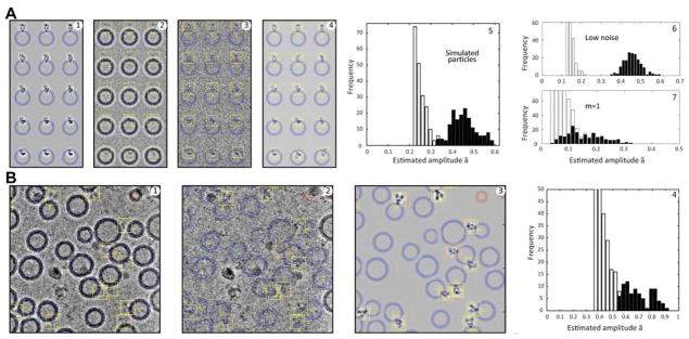
Automatic particle detection from simulated and experimental images. (A1) Simulated merged images of GluA2 particles with the same CTF and pre-whitening filter as employed with the experimental micrograph in Fig. 6. (A2) The image after adding white Gaussian noise. (A3) The residual after subtract-ing fitted vesicles. The blue rings indicate the location of the subtracted vesicle density. (A4) The best-matching references S̃k. A total of 3856 references were calculated from projections of the X-ray structure with an angular sampling of about 15°; nl = 32 references (8 values of the angle γ) were considered at each pixel position, and m = 20 terms were used in the image expansions. Yellow boxes indicated the detected particles. (A5) A histogram of the estimated amplitude values ã for true particles (black bars) and false positives (white bars). The white bars extend only to the value of 0.21 which was the lowest threshold that was tested; a threshold of 0.35 for ã would result in nearly perfect discrimination between true and false particles and is the threshold used in particle detection in panels A1–A4. (A6) The result of automatic particle detection when the noise standard deviation is reduced to half; the false and true particle peaks are widely separated. (A7) A histogram showing the poor detection results when a single reference is used, that is when the number of terms m is set to 1. (B1) A portion of the micrograph shown in Fig. 6 with automatically-detected particles marked. Yellow boxes indicate correctly-identified particles, and an orange box indicates a false particle that was detected, probably an ice ball. (B2) is the corresponding residual image with vesicle membranes subtracted. (B3) The best-matching references are shown. (B4) The histogram of signal amplitudes in the entire micrograph, with black bars indicating the 66 visually-identified true particles. A threshold of 0.53 for ã results in apparently ideal particle discrimination. The references shown in Fig. 4B are members of the set of references used for particle selection in both parts A and B of this figure.
The processing of an actual micrograph is demonstrated in Fig. 7B. All but one of the detected particles (boxes) visually matches the reference. The one questionable particle (more likely a small ice ball) that was detected is marked with an orange box. Although there is no “ground truth” in this case, the histogram of ã values (Fig. 7B4) appears to show a separation of true and false particles like that seen in the simulation.
4. Discussion
We describe here a geometry-aware particle picker for lipid-vesicle-embedded membrane proteins. At each pixel position the particle-selection algorithm tests for the existence of a particle whose center of mass lies on that position. In this process only those reference images (projections of a 3D particle model) are considered that are appropriate to that pixel location in view of the constraint that the particle is oriented normal to the membrane surface. The expansion of each reference image in a set of basis images makes for the very efficient calculation (Eq. (9)) of the cross-correlation while using position-dependent sets of references.
The GluA2 particles, which are considered here as a test case, are particularly challenging for template-based particle detection because their extended shape presents very different 2D projections depending on the viewing direction. Indeed, the discrimination of true from false particles is much worse if a single average reference projection is used (compare Fig. 7A5 and Fig. 7A7). This arises because one term is insufficient, while ~20 terms in the eigenimage expansion capture most of the power in the thousands of possible references (Fig. 3C). Using this expansion, and tested with simulated images and actual micrographs, the algorithm provides reliable detection of these 400 kDa membrane-protein particles in images taken with a conventional CCD camera.
Acknowledgments
We thank K. Duerr and E. Gouaux (Vollum Institute, Portland, OR) for the purified GluA2 protein, Y-Y. Yan and Y. Yang for reconstituting it into lipid vesicles, and H. Shigematsu for cryo-EM imaging. We are grateful to H. Tagare and A. Barthel for helpful discussions. This work was supported by NIH grant R01NS21501 to F.S.
Footnotes
Publisher's Disclaimer: This is a PDF file of an unedited manuscript that has been accepted for publication. As a service to our customers we are providing this early version of the manuscript. The manuscript will undergo copyediting, typesetting, and review of the resulting proof before it is published in its final citable form. Please note that during the production process errors may be discovered which could affect the content, and all legal disclaimers that apply to the journal pertain.
References
- Jiang QX, Chester DW, Sigworth FJ. Spherical Reconstruction: A Method for Structure Determination of Membrane Proteins from Cryo-EM Images. J Struct Biol. 2001;133(2–3):119–131. doi: 10.1006/jsbi.2001.4376. [DOI] [PubMed] [Google Scholar]
- Wang L, Sigworth FJ. Liposomes on a streptavidin crystal: a system to study membrane proteins by cryo-EM. Methods Enzymol. 2010;481:147–164. doi: 10.1016/S0076-6879(10)81007-9. [DOI] [PMC free article] [PubMed] [Google Scholar]
- Roseman AM. Particle finding in electron micrographs using a fast local correlation algorithm. Ultramicroscopy. 2003;94:225–236. doi: 10.1016/s0304-3991(02)00333-9. http://dx.doi.org/10.1016/S0304-3991(02)00333-9. [DOI] [PubMed] [Google Scholar]
- Zhu Y, Carragher B, Glaeser RM, Fellmann D, Bajaj C, Bern M, Mouche F, de Haas F, Hall RJ, Kriegman DJ, Ludtke SJ, Mallick SP, Penczek PA, Roseman AM, Sigworth FJ, Volkmann N, Potter CS. Automatic particle selection: results of a comparative study. J Struct Biol. 2004;145:3–14. doi: 10.1016/j.jsb.2003.09.033. http://dx.doi.org/10.1016/j.jsb.2003.09.033. [DOI] [PubMed] [Google Scholar]
- Voss N, Yoshioka C, Radermacher M, Potter C, Carragher B. DoG Picker and TiltPicker: Software tools to facilitate particle selection in single particle electron microscopy. J Struct Biol. 2009;166(2):205–213. doi: 10.1016/j.jsb.2009.01.004. http://dx.doi.org/10.1016/j.jsb.2009.01.004. [DOI] [PMC free article] [PubMed] [Google Scholar]
- Chen JZ, Grigorieff N. SIGNATURE: A single-particle selection system for molecular electron microscopy. J Struct Biol. 2007;157(1):168–173. doi: 10.1016/j.jsb.2006.06.001. http://dx.doi.org/10.1016/j.jsb.2006.06.001. [DOI] [PubMed] [Google Scholar]
- Langlois R, Pallesen J, Frank J. Reference-free particle selection enhanced with semi-supervised machine learning for cryo-electron microscopy. J Struct Biol. 2011;175:353–361. doi: 10.1016/j.jsb.2011.06.004. http://dx.doi.org/10.1016/j.jsb.2011.06.004. [DOI] [PMC free article] [PubMed] [Google Scholar]
- Sigworth FJ. Classical detection theory and the cryo-EM particle selection problem. J Struct Biol. 2004;145(1–2):111–122. doi: 10.1016/j.jsb.2003.10.025. [DOI] [PubMed] [Google Scholar]
- Sobolevsky AI, Rosconi MP, Gouaux E. X-ray structure, symmetry and mechanism of an AMPA-subtype glutamate receptor. Nature. 2009;462(7274):745–756. doi: 10.1038/nature08624. [DOI] [PMC free article] [PubMed] [Google Scholar]
- Heymann JB, Chagoyen M, Belnap DM. Common conventions for interchange and archiving of three-dimensional electron microscopy information in structural biology. J Struct Biol. 2005;151(2):196–207. doi: 10.1016/j.jsb.2005.06.001. [DOI] [PubMed] [Google Scholar]
- Wang L, Bose PS, Sigworth FJ. Using cryo-EM to measure the dipole potential of a lipid membrane. Proc Natl Acad Sci U S A. 2006;103(49):18528–18533. doi: 10.1073/pnas.0608714103. [DOI] [PMC free article] [PubMed] [Google Scholar]
- Huang Z, Penczek PA. Application of template matching technique to particle detection in electron micrographs. J Struct Biol. 2004;145:29–40. doi: 10.1016/j.jsb.2003.11.004. http://dx.doi.org/10.1016/j.jsb.2003.11.004. [DOI] [PubMed] [Google Scholar]
- Kirkland EJ. Advanced Computing in Electron Microscopy. 1. Plenum Press; New York: 1998. [Google Scholar]
- Shang Z, Sigworth FJ. Hydration-layer models for cryo-EM image simulation. J Struct Biol. 2012;180(1):10–16. doi: 10.1016/j.jsb.2012.04.021. http://dx.doi.org/10.1016/j.jsb.2012.04.021. [DOI] [PMC free article] [PubMed] [Google Scholar]
- Zeng X, Stahlberg H, Grigorieff N. A maximum likelihood approach to two-dimensional crystals. J Struct Biol. 2007;160(3):362–374. doi: 10.1016/j.jsb.2007.09.013. http://dx.doi.org/10.1016/j.jsb.2007.09.013. [DOI] [PMC free article] [PubMed] [Google Scholar]
- Baxter WT, Grassucci RA, Gao H, Frank J. Determination of signal-to-noise ratios and spectral SNRs in cryo-EM low-dose imaging of molecules. J Struct Biol. 2009;166(2):126–132. doi: 10.1016/j.jsb.2009.02.012. http://dx.doi.org/10.1016/j.jsb.2009.02.012. [DOI] [PMC free article] [PubMed] [Google Scholar]
- Langlois R, Frank J. A clarification of the terms used in comparing semi-automated particle selection algorithms in Cryo-EM. J Struct Biol. 2011;175:348–352. doi: 10.1016/j.jsb.2011.03.009. http://dx.doi.org/10.1016/j.jsb.2011.03.009. [DOI] [PMC free article] [PubMed] [Google Scholar]