

Abstract
We give critical attention to the assumptions underlying Mendelian randomization analysis and their biological plausibility. Several scenarios violating the Mendelian randomization assumptions are described, including settings with inadequate phenotype definition, the setting of time-varying exposures, the presence of gene-environment interaction, the existence of measurement error, the possibility of reverse causation, and the presence of linkage disequilibrium. Data analysis examples are given illustrating that the inappropriate use of instrumental variable techniques when the Mendelian randomization assumptions are violated can lead to biases of enormous magnitude. To help address some of the strong assumptions being made, three possible approaches are suggested. First, the original proposal of Katan (Lancet. 1986; 1:507-508) for Mendelian randomization was not to use instrumental variable techniques to obtain estimates, but merely to examine genotype-outcome associations to test for the presence of an effect of the exposure on the outcome. We show that this more modest goal and approach can circumvent many, though not all of, the potential biases described. Second, we discuss the use of sensitivity analysis in evaluating the consequences of violations in the assumptions and attempts to correct for those violations. Third, we suggest that a focus on negative, rather than positive, Mendelian randomization results may turn out to be more reliable.
There has been increasing interest in Mendelian randomization as a way to assess causal effects.1-19 The basic idea of this approach is to use a genetic marker that affects a particular exposure, and affects an outcome of interest only through the exposure. The effect of the genetic marker on the exposure and on the outcomes is then used to back out the effect of the exposure itself on the outcome. Under assumptions described below, this can be done even if the exposure-outcome relationship itself is confounded. This approach essentially uses the genetic marker as an “instrumental variable”3-5,9,10 for the effect of the exposure on the outcome. Under exposure-outcome confounding, where associations between the exposure and the outcome do not themselves reflect causal effects, the Mendelian randomization approach can still estimate these causal effects. The approach is appealing because in many settings the confounding between the exposure and the outcome may be intractable so that causal effects cannot be estimated from observational data using standard regression techniques.
The Mendelian randomization approach, however, itself makes a number of assumptions and these assumptions are not always carefully evaluated. Stated informally, these assumptions are that (1) the genetic marker is associated with the exposure, (2) the genetic marker is independent of the outcome given the exposure and all confounders (measured and unmeasured) of the exposure-outcome association, and (3) the genetic marker is independent of factors (measured and unmeasured) that confound the exposure-outcome relationship. The second assumption is sometimes referred to as the exclusion restriction; if the genetic marker affects the exposure then, the assumption is also sometimes stated as the genetic marker affecting the outcome only through the exposure. In other words, for the assumptions of Mendelian randomization to hold, we need a setting like that of Figures 1A or 1B. The Mendelian randomization assumptions are violated in a diagram like that of Figure 2A or 2B because the genetic marker affects the outcome through pathways other than through the exposure.
Figure 1.

Diagrams illustrating a genetic variant (G) which is an instrument for the effect of exposure (X) on outcome (Y) when the exposure-outcome relationship is confounded by unmeasured factors (U)
Figure 2.

Diagrams illustrating violations of the exclusion restriction with the genetic variant (G) not independent of outcome (Y) conditional on exposure (X) and confounders (U) because of a direct effect of G on Y not through X
If these assumptions do hold, then methods from the instrumental variable literature9-11 can be applied to use data on the genetic marker, the exposure and the outcome to estimate the effect of the exposure on the outcome. It is not necessary to have information on the exposure-outcome confounders themselves to be able to do this. If assumption (1) holds but the association between the genetic marker and the exposure is weak, then the genetic marker is sometimes referred to as a “weak instrument.” Using a weak instrument will often amplify biases due to any violations in the other two Mendelian randomization assumptions.
Although there may be general awareness that these assumptions must hold in a Mendelian randomization analysis, we believe insufficient attention is paid to evaluating these assumptions and their implications. We will discuss these assumptions and their implications. We will argue that in a number of genetic contexts these assumptions are not plausible. We will also present three ways to help address some of these assumptions and their potential violations, which we believe would help strengthen inferences from Mendelian randomization analyses.
Exclusion Restriction Violations: Pathways, Time, Interaction, Measurement Error, Reverse Causation, Sample Selection, and Linkage Disequilibrium
We first highlight ways in which the exclusion restriction might be violated. First, if the genetic marker is not to affect the outcome except through the exposure, then the exposure that is used in the analysis must capture all of the ways that the genetic marker may be associated with the outcome. Consider a setting such as that in Figure 3 where G denotes the genetic marker, X the exposure of interest used in the analysis and Y the outcome. Let W be some variable that is on the pathway from the genetic marker G to the exposure X. In this case, if X is used as the exposure in the analysis, the Mendelian randomization approach will be biased. This is because the genetic marker affects the outcome through a pathway that does not go through the exposure X, namely, G→W→Y. For the assumptions of the Mendelian randomization analysis to hold, then the exposure X must be the first and only variable on the pathway from G to Y. If there were any variable W on the pathway from G to X that also affected Y, the Mendelian randomization analysis would be biased.
Figure 3.

Setting in which the variant (G) affects an intermediate (W) on the pathway to exposure (X), violating the exclusion restriction
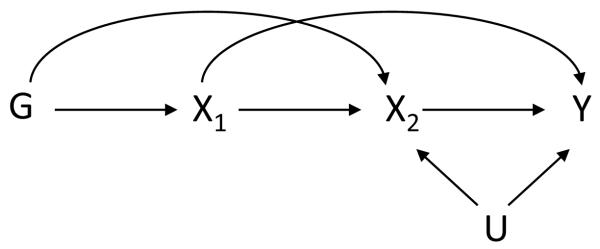
Consider a closely related scenario (Figure 4). Suppose that the genetic marker affects the outcome only through a particular exposure or phenotype, but that this itself consists of two components (X1,X2). If only one of these two components, X1 say, were used in the Mendelian randomization analysis, then there could be substantial bias in the Mendelian randomization estimates of the effect of the exposure on the outcome. Once again, the exclusion restriction is violated: the genetic marker affects the outcome via pathways other than the exposure X1 used in the analysis. The results of the Mendelian randomization analysis will be biased for the effects of X1 on Y and also for the effects of (X1,X2) on Y.
Figure 4.

Setting in which the exclusion restriction holds when (X1, X2) are taken together as the exposure but does not hold for X1 alone.
A related case in this scenario might be if X1 and X2 constitute the exposure of interest at two different times (Figure 5), both of which can affect the outcome Y. If the measurement at only one of the times is used in the analysis, then once again the Mendelian randomization analysis will be biased.
Figure 5.
Setting in which the exposure is time-varying and in which the exclusion restriction holds when (X1, X2) are taken together as the exposure but does not hold for X1 alone.
Many of these points have been acknowledged,3, 5, 9 but it is not clear that these issues are seriously evaluated and discussed when Mendelian randomization analyses are carried out in practice. It is sometimes claimed that, although the Mendelian randomization assumptions may not hold exactly, the bias resulting from them is likely to be small in comparison with the bias from simply examining the associations between the exposure and the outcome.3 While this claim may hold in some scenarios, it certainly will not hold in all. Violations of the exclusion restriction, such as we have discussed, can in fact lead to substantial biases in Mendelian randomization analysis. We illustrate with an example.
It has recently been established that genetic variants on chromosome 15 affect both smoking behavior (e.g. cigarettes per day) and lung cancer. Subsequently there has been interest as to whether the effects of the variants on lung cancer operate entirely through smoking or whether they might also operate through other pathways. A recent analysis20 using lung cancer case-control data to examine whether there were additional pathways (not through increasing cigarettes per day) provided substantial evidence that such pathways were indeed present. The techniques employed in this analysis were mediation techniques21-23 rather than Mendelian randomization techniques; i.e. they did not assume (as Mendelian randomization analysis does) that there were no pathways of the variants on lung cancer except through cigarettes per day. Instead, the techniques were designed to evaluate this assumption. The results of these analyses established the presence of pathways other than through increasing cigarettes per day, and showed that in fact most of the effect of the variants on lung cancer were not due to increasing cigarettes per day. Extensive sensitivity analyses for unmeasured confounding and measurement error confirmed this, and the results have been replicated in three other studies.20
Note, however, that the mediator being evaluated was only cigarettes per day, not all aspects of smoking. The results of the analysis are thus still consistent with the possibility that smoking behavior, taken as a whole, mediates the entirety of the association. Indeed it has been suggested24 that a central means by which the variants affect lung cancer is by increasing the amount of nicotine and toxins extracted per cigarette (e.g. through deeper inhalation). This then would be a scenario similar to that depicted in Figure 4, where two aspects of the smoking phenotype (e.g. cigarettes per day X2 and depth of inhalation X1) may mediate all of the effect. What happens then if one were to apply Mendelian randomization using only cigarettes per day? The Mendelian randomization assumptions would be violated because there are other pathways from the variants to lung cancer. In this case, as we will see below, the biases can be substantial.
Using the same lung cancer data, the crude association between smoking one pack of cigarettes per day and lung cancer has an odds ratio of 2.6 (95% confidence interval [CI] = 2.3 - 3.0) controlling for age, sex, and college education. If we apply a Mendelian randomization approach19 to these data, taking cigarettes per day as our exposure, we obtain an odds ratio for the effect of a pack of cigarettes per day on lung cancer of 2,180 - vastly larger than that from examining the smoking-lung cancer association directly. Although the smoking-lung cancer association may be confounded, it is unlikely that it could be confounded to the degree that would be required for an effect estimate odds ratio of 2,180. In this case, the bias arises from the Mendelian randomization due to a failure of the exclusion restriction. The estimate is severely exaggerated because the exposure variable used – cigarettes per day – captures only a small part of the effect of genetic variants on the outcome (i.e. the exclusion restriction is violated). Moreover, the association between the variant and cigarettes per day is relatively weak, resulting in weak instrument problems, which amplifies the bias due to the exclusion restriction violation. The Mendelian randomization estimate for the effect of cigarettes per day on lung cancer effectively divides the variant-lung cancer association by the variant-cigarettes association; because the latter is so small (since cigarettes per day is only one aspect of smoking by which the variants may affect lung cancer), the final Mendelian randomization estimate is biased dramatically upwards.
This example also suggests another way in which the exclusion restriction can be violated. The effects of the variants on lung cancer can be understood as an amplification of the effect of each cigarette smoked (because those with the variant extract more nicotine and toxins per cigarette).24 This is a form of gene-environment interaction, and indeed there is strong statistical evidence for such gene-environment interaction (between the variants and cigarettes per day) on both the additive and multiplicative scales.20 However, gene-environment interaction (when both the genetic factor and the environmental factor cause the outcome and interact in their effects) itself constitutes a violation of the exclusion restriction. This is because under such gene-environment interaction, the genetic variants affects the outcome not simply through the value the exposure takes. Such interaction corresponds to Figure 2A, not to Figure 1A. Figure 1A requires that once we know the exposure X, the genetic marker G gives us no further information about the outcome Y. In the presence of gene-environment interaction, this does not hold, and Figure 2A would describe the actual relations. The exclusion restriction is thus again violated, and Mendelian randomization analyses are shown to be biased. It is important to keep in mind that gene-environment interaction may depend on how the exposure is defined. If the exposure were defined as all aspects of smoking behavior (or a composite measure of nicotine and toxins extracted), there may be no gene-environment interaction. The genetic variants may affect lung cancer only through the composite of all aspects of smoking behavior. However, when the exposure is defined as cigarettes per day, then gene-environment interaction is present and the exclusion restriction is violated. Instrumental variable methods allowing for interaction can, in some contexts, be employed,25, 26 but the assumptions underlying the use of standard instrumental variable estimators would in general be violated in the presence of gene-environment interaction.
This brings us to yet another potential violation of the exclusion restriction. Consider the diagram in Figure 6, in which the exclusion restriction holds for the true underlying exposure X, but the investigator has access only to X*, a measure of the exposure subject to measurement error. Here again, the exclusion restriction will in general be violated. Some specific exceptions can arise, such as when the exposure X is continuous and subject to classical non-differential measurement.3, 10, 16, 17, 25 However, in other cases, such as with a dichotomous exposure or differential measurement error, Mendelian randomization analyses will be biased. It is moreover possible that the disease itself distorts the measurement of the exposure with an arrow from Y to X* in Figure 6. This would introduce still more bias.
Figure 6.

Diagram illustrating that when the exposure (X) is measured with error (X*) the exclusion restriction will not in general hold for the mismeasured exposure X*
This brings us to yet another possible violation of the exclusion restriction, which is through reverse causation or feedback. Consider the diagram in Figure 7 in which the genetic variant has no effect on the outcome Y1 that does not go through the exposure (X0,X1) but the exposure X1 is affected by the prior outcome Y0. If in a Mendelian randomization analysis (X0,X1) is used as the exposure with the outcome Y1, then our Mendelian randomization assumptions will be violated. In this case the genetic marker G is not independent of the outcome Y1 conditional on the exposure (X0,X1) and the confounders U, since conditional on (X0,X1,U), the variant G is still associated with Y1 through the path G→X1←Y0→Y1 which is open, conditional on X1. We would thus get biased estimates when using instrumental variable techniques to estimate the effect of (X0,X1) on Y1. We note that the situation described in Figure 7 is especially worrisome for retrospective case-control studies, where data on the exposure is collected after diagnosis of the outcome.
Figure 7.

Setting in which prior outcome (Y0) can affect subsequent exposure (X1) so that the variant (G) is not independent of final outcome (Y1) conditional on exposures (X0,X1) and confounders (U), violating MR assumptions, due to reverse causation
Violations of the exclusion restriction can also arise due to the selection of the sample. For example, if interest lies in the effect of X on Y but the sample was originally collected as part of a case-control study of another disease D and both Y and X are associated with D (Figure 8), then even though there is no effect of G on Y that does not go not through X, G is still associated with Y conditional on exposure X and confounders U because of the conditioning on the status of D. Instrumental variable estimates of the effect of X on Y will again be biased. Existing case-control studies are increasingly used for Mendelian randomization analyses of traits other than the diseases they were originally designed to study, so this scenario is relevant in practice. Methods for handling Mendelian randomization analyses with such secondary phenotypes are becoming available,27 but if the design is ignored when using standard methods, then biased estimates will result.
Figure 8.

Setting in which variant (G) is associated with outcome (Y) conditional on exposure (X) and confounders (U), violating the MR assumptions, because of using data from a case-control study of another outcome (D)
Finally, consider the diagram in Figure 9 in which another genetic marker GU, which also affects the outcome Y, is in linkage disequilibrium with the genetic marker G used in the analysis. This again constitutes a violation of the exclusion restriction because G is not independent of Y conditional on X and U. That such linkage disequilibrium violates the assumptions of a Mendelian randomization analysis has been noted in principle,3, 9 but is seldom discussed in practice. In this case, we could restore the Mendelian randomization assumptions if we could control for the other genetic marker GU. However, to entirely avoid such violations, like that in Figure 9, it would be required that there be nothing on the same chromosome as the genetic marker used in the analysis that also affects the outcome, or that all such variables be controlled. This is a strong assumption and potential violations are numerous. Recent large-scale fine-mapping studies of auto-immune disease, metabolic traits, cancers, and anthropometric traits have all identified risk loci containing multiple correlated alleles that remain statistically significantly associated with these outcomes after mutual adjustment.28-32 Moreover, there are many loci that harbor distinct, linked alleles associated with a wide range of phenotypes (e.g. the HLA region and the ABO locus).33, 34 As a concrete example, Garcia-Closas et al.35 report evidence for a variant for body mass index (BMI) in the FTO gene that is strongly correlated with a different variant for breast cancer. If this variant for BMI were used in a Mendelian randomization analysis for the effect of BMI on breast cancer, the Mendelian randomization assumptions would be violated.
Figure 9.

Setting in which variant (G) is associated with outcome (Y) conditional on exposure (X) and confounders (U), violating MR assumptions, because of linkage disequilibrium with another variant (GU) that affects the outcome.
Similar violations of the exclusion restriction occur in the presence of population stratification. Although this can be addressed using the standard methods of genomic control employed in genome-wide association studies, or by using family-based studies,34, 10 such methods are not necessarily being employed in Mendelian randomization studies. Failure to do so would result in a causal diagram similar to Figure 9, with biased results.
These points are not new, but are they adequately considered when Mendelian randomization is employed in practice. Furthermore, violations can potentially lead to substantial biases. When reporting results of a Mendelian randomization analysis, investigators should clearly state the assumptions being made in the context of their specific application, and should discuss the plausibility of the assumptions. Investigators should consider and comment on (1) whether the exposure used in the analysis completely captures the phenotype that may mediate the association between the variant and the outcome, (2) whether the exposure is time-varying, (3) whether there may be gene-environment interaction, (4) whether the exposure may be measured with error, (5) whether there may be reverse causation, and (6) whether there may be other genetic markers on the same chromosome that affect the outcome and are correlated with the marker used in analysis. If a good argument can be made against these possibilities then investigators can more reliably assume that the exclusion restriction holds. These are, of course, all very strong assumptions. Is there another way forward?
Approach 1 - A Return to Katan
The origin of Mendelian randomization analysis is often traced to a letter by Katan.1 Katan did not propose using instrumental variable statistical methods to estimate the effect of the exposure on the outcome. Rather, he simply proposed examining the association between the genetic variants and the outcome to test for an effect of the exposure on the outcome. He proposed not using the exposure data at all!
At first this may be surprising. It would seem that we should be better off making use of the exposure data. However, as discussed in the previous section, one of the challenges in ensuring that the exclusion restriction holds is defining and measuring the exposure in such a way as to avoid incomplete phenotype information (time-varying or otherwise), measurement error, and gene-environment interaction. This will, in general, not be easy to do. However, if all we are interested in is testing for an effect of the exposure on the outcome (rather than estimating the magnitude of this effect), then no exposure information is needed. We need only data on the genetic variant and the outcome. We still need to make the exclusion restriction assumption – that the variant affects the outcome only through the exposure – but we do not necessarily need to fully specify what that exposure is, or collect data on the exposure thus defined. To see this, consider again the diagrams in Figures 1A and 1B. If there were no effect of the exposure on the outcome (i.e. no arrow from X to Y), then the genetic variant G and the outcome Y should be unassociated. If there is no arrow from G directly to Y (i.e. if the exclusion restriction holds) and if G and Y are correlated, then there must be an effect of the exposure X on the outcome Y. And we can test for this without using data on X. This was the approach initially proposed by Katan.
Of course it seems more desirable to obtain estimates of the effect of the exposure on the outcome rather, than just to test for the presence of an effect. That is what the instrumental variable methods used in Mendelian randomization analysis purportedly do. However, doing so requires much stronger assumptions. This is because for tests to be valid we need the Mendelian randomization to hold under some definition of the exposure. For valid estimates we need the Mendelian randomization assumption to hold for the measurement of the exposure for which data is available. The Mendelian randomization assumptions are much less likely to hold for a single measurement of the exposure than they are for a complete characterization of all aspects of the exposure and exposure history. If we had data on the entire history of all aspects of the exposure, then we could potentially again proceed to obtain estimates using causal assumptions no stronger than those involved in the tests. In the absence of such complete exposure data, however, the tests require weaker assumptions than the estimates.
Let us revisit the potential violations of the exclusion restriction in Figures 4-9. Suppose we were to follow the original approach proposed by Katan. Consider Figure 4 and suppose we had data only on X1. As discussed above, our Mendelian randomization estimates would be biased. However, if we were to simply examine whether there was association between G and Y, we would still have a valid test of whether there was an effect of phenotype (X1, X2) on the outcome Y. If there was no effect, then we should observe no association between G and Y. Likewise in Figure 5, with time-varying exposures, we could test whether there were an effect of the exposure (X1, X2) on the outcome Y by testing whether G and Y were associated. Once again, if there were no effect, then we should observe no association between G and Y. The difficulties with observing only part of the relevant phenotype vanish. We do not need exposure/phenotype information, and we are protected against the biases described earlier because we are not estimating but rather testing.
Similarly, in the case of gene-environment interaction, if there were some definition of the phenotype such that there was no gene-environment interaction (i.e. once the phenotype is known, the genetic marker gives no further information on the outcome) so that Figure 1A or 1B holds for that definition of phenotype rather than Figure 2a or 2b, then we could once again test for an effect of phenotype on outcome simply by looking at the association between the genetic marker and the outcome. If there were no effect, we should find no association. Note that here we do not even need to know under what definition of the phenotype there would be no gene-environment interaction; we only need to assume that there is one and that, with respect to this definition, the exclusion restriction holds.
Similar conclusions hold in the case of measurement error. If we use the original approach suggested by Katan, measurement error does not cause a problem. In Figure 6, if there is no effect of the true exposure X on Y, we should find no association between G and Y. We can do testing without data on X without worry about measurement error in X. Similarly with Figure 7, if X1 and Y1 were associated only because of reverse causation (i.e. because Y0 affects both X1 and Y1, as in Figure 7, rather than because X affects Y), then we would find no association between G and Y1 if there were no arrow from (X0,X1) to (Y0,Y1).
The approach of Katan is thus robust to many of the sources of bias and exclusion restriction violations considered in the previous section, because no data on the exposure is needed to proceed with testing. The price of this robustness is that we get only tests, not estimates. The approach of using just the genetic marker and the outcome to test for an effect of the exposure on the outcome is, however, not robust to all forms of exclusion restriction violations. In Figures 2 or 3, the exclusion restriction would be violated for the exposure X, and both tests (using the approach of Katan) and estimates (using instrumental variable methods) would be biased. Likewise in Figure 8, in which there is selection bias or in Figure 9, in which another variant that affects the outcome is in linkage disequilibrium with the variant used in the analysis, the assumptions are violated, and both tests and estimates will be biased.
Still, tests are often protected when estimates are not (Figures 4-7). Testing with Mendelian randomization can be seen as analoguous to intent-to-treat analysis in randomized trials in the presence of non-compliance. In trials with non-compliance, we can still get unbiased estimates of the intent-to-treat effect by simply comparing outcomes according to treatment assignment – this is the effect of treatment assignment. However, if we want to estimate the effect of actually complying with the treatment, then we must take non-compliance into account. This is sometimes done using instrumental variable methods, with treatment assignment taken as an instrument for compliance/treatment taken. Doing so requires making the exclusion restriction assumption (i.e. there is no effect of assignment on outcome that does not go through measured treatment taken). We may be worried that such an assumption is violated (due to mismeasured compliance, partial compliance, or psychological effects of treatment assignment) and so standard practice in randomized trials is to take the intent-to-treat effect as the primary estimate of the study and to make an instrumental variable analysis (or any other analysis using compliance data) as a secondary analysis. This ensures the greatest validity for the primary analysis. The equivalent to the intent-to-treat analysis in Mendelian randomization is to simply look at the G-Y association, which is the original approach of Katan. Current Mendelian randomization practice is to report instrumental variable estimates as primary, but perhaps this should be reversed, with testing as primary and the instrumental variable estimate as secondary, thereby paralleling practices in randomized trials.
The other thing that is made clear by the approach of Katan is the strength of the assumptions. We are using a test of association between the genetic marker and the outcome to draw a conclusion about the effect of the exposure on the outcome. The assumptions being made, as outlined above, do the rest of the work. Testing for association between the genetic marker and the outcome makes these strong assumptions more clear. It should also be noted that the instrument variable methods themselves could in theory be used only for the purposes of testing. Testing whether the instrumental variable estimate is different from zero constitutes a valid test of the null hypothesis of no association between the genetic variant and the outcome, and thus under the Mendelian randomization assumptions a valid test of the null of no effect of the exposure on the outcome.9 Such a test makes no stronger causal assumptions than the approach of Katan. It is when the instrument variable techniques are used to obtain estimates, rather than just tests, that the stronger assumptions (concerning the validity of the exclusion restriction for the actual exposure measured) are required. But if instrumental variable methods are being used only for testing, it is not clear why they would be preferred to the approach advocated by Katan. In using instrumental variable methods, it can seem that the sophistication of the analysis somehow produces the conclusion, whereas in fact, it is relying on assumptions - and even stronger assumptions for estimation.
Approach 2 - Sensitivity Analysis for the Exclusion Restriction and Other Violations
Although the approach of Katan can be helpful in addressing violations of the Mendelian randomization assumptions in Figures 4-7, some of the other violations, such as those in Figures 2, 3, 8 and 9, are still subject to bias. Another approach to help address violations of the Mendelian randomization assumptions is to use sensitivity analysis to assess the extent to which various exclusion restriction violations or assumption violations due to linkage disequilibrium with another variant affecting the outcome (or population stratification) would bias results, and then to try to correct for such bias. The techniques can be adapted in a straightforward manner from existing sensitivity analysis techniques in the literature.36-38 We present sensitivity analysis techniques for the approach of Katan; in the Appendix we discuss how these can also be applied also to instrumental variable estimation.
Consider Figure 10, in which we have both a violation of the exclusion restriction (an arrow for G to Y not through X) and linkage disequilibrium (another genetic marker GU that was in linkage disequilibrium with G and affected the outcome Y). Suppose first that the outcome Y is dichotomous and we are comparing two levels of the genetic marker G (G=0 and G=1). Suppose then that we estimate a risk ratio between G and Y possibly conditional on measured baseline covariates (which could be approximated by an odds ratio using logistic regression if the outcome is rare). Suppose we assume GU is binary and does not interact with G on the risk-ratio scale in its effects on Y and that GU increases the risk of Y by a factor of γ on the risk-ratio scale. Suppose also that although the exclusion restriction is violated (i.e. there is a path from G to Y not through X), that the effects of G and X on Y do not themselves interact on the risk ratio scale; and that the effect of the direct path from X to Y is to increase the risk of Y by a factor of λ on the risk ratio scale. Under these assumptions, we can obtain a “corrected” estimate and confidence interval for the association between G and Y (i.e. what we would have obtained had we been able to control for GU and had we been able to isolate the G→X→Y path) by dividing our observed estimate and confidence interval by λ{1+(γ-1)π1}/{1+(γ - 1)π0}36,38 where π1 and π0 are the prevalences of GU among those with G=1 and those with G=0, respectively. We could specify values of λ, γ, π1 and π0 based on prior studies or we could consider a range of these values and vary them in a sensitivity analysis. Doing so would allow one to assess the degree of confounding by another genetic variant and the strength of the exclusion restriction violations that would be required to explain away the association between the genetic variant G and the outcome Y that is used to test for an effect of the exposure on the outcome. Values of the sensitivity analysis parameters for which the null was still not rejected would be those for which there was still evidence of a causal effect of exposure X on outcome Y, even though the assumptions themselves were violated.
Figure 10.

Setting in which variant (G) is associated with outcome (Y) conditional on exposure (X) and confounders (U), violating MR assumptions, because of linkage disequilibrium with another variant (GU) that affects the outcome, and in which the exclusion restriction is violated.
Likewise for a continuous outcome, Y, suppose we estimate the effect of G on Y on the difference scale, possibly conditional on measured baseline covariates. Suppose we assume GU is binary and does not interact with G on the additive scale in its effects on Y and that GU increases Y on average by a difference of γ. Suppose also that, although the exclusion restriction is violated, the effects of G and X on Y do not themselves interact on the difference scale, and the effect of the direct path from X to Y is to increase the average value of Y by a difference of λ. Under these assumptions, we can obtain a “corrected” estimate and confidence interval (i.e. what we would have obtained had we been able to control for GU and had we been able to isolate the G X Y path so that the exclusion restriction was not violated) by subtracting from our observed estimate and confidence interval the factor γδ+λ where δ is the difference in the prevalences of GU among those with G=1 and those with G=0, respectively.36,38 If GU is specified as continuous rather than binary, then γ can be modified to the effect of a one-unit increase in GU on Y, and δ can be modified to the difference in means of GU among those with G=1 versus G=0.38 We could again specify values of γ and δ based on prior studies or we could consider a range of these values and vary them in a sensitivity analysis. Again, doing so would allow one to assess the degree of confounding by another genetic variant and the strength of the exclusion restriction violations that would be required to explain away the association between the genetic variant G and the outcome Y that is used to test for an effect of the exposure on the outcome.36-38 Values of the sensitivity analysis parameters for which the null was still not rejected would be those for which there was still evidence of a causal effect of exposure X on outcome Y, even though the assumptions themselves were violated.
While the approach of Katan is subject to bias by linkage disequilibrium with another variant that affects the outcome, as well as to some of exclusion restriction violations, the extent of this bias can be assessed through sensitivity analysis.
Approach 3 - Negative Results May Be More Plausible
The assumptions required for Mendelian randomization are strong, whether for estimation or for testing. The number of applications of Mendelian randomization has been quickly expanding. More attention needs to be paid to its assumptions – to whether incomplete exposure information, time-varying exposures, gene-environment interaction, measurement error, reverse causation, or linkage disequilibrium might bias the analysis. Employing the approach of Katan for testing, rather than estimation, circumvents some of these biases, but not others. It is in general difficult to establish with much certainty the exclusion restriction that is required in these analyses. Although empirical tests exist to falsify these assumptions,17, 25, 39-40 the assumptions cannot be fully empirically verified.
In light of the strength of the assumptions being made, it may turn out that Mendelian randomization analysis is more important for establishing negative results. If there is no association between the genetic variant and the outcome, and if it has already been established that the variant affects the exposure of interest, then this would provide evidence that there is in fact no or very little effect of the exposure on the outcome. Of course, relatively large sample sizes would be needed to establish a null or near-null association with confidence. It would also be necessary to use genetic variants strongly associated with the exposure to avoid weak-instrument problems.4 However, research consortia are making it more and more possible to achieve such large sample sizes.
Negative results, like positive results, are potentially subject to biases arising from violations in the assumptions. However, the biases would have to all align perfectly in order to move the effect estimate to zero when there is in fact a true effect. There is the whole range of non-zero values for false positives to take; there is only one zero value that a false negative may take. A null association, with narrow confidence interval, between a genetic variant and an outcome may thus arguably provide more robust evidence of the negative conclusion of no or very little effect. Such null results can also address important clinical and etiological questions. One recent example is the finding that CRP-associated variants are not associated with coronary heart disease (suggesting that CRP is not causally associated with heart disease). Another example are results that indicate that BMI-associated variants are associated with circulating vitamin D levels, while variants associated with vitamin D levels are not associated with BMI (suggesting BMI is causally associated with vitamin D levels but not vice versa).41, 42 In light of the strength of the assumptions and the asymmetry between false negative and false positives, Mendelian randomization may in the end prove most valuable in establishing that certain exposures do not affect outcomes, rather than that they do.
Acknowledgements
Tyler J. VanderWeele was supported by National Institutes of Health grant ES017876.
Appendix. Sensitivity Analysis for Violations of the Mendelian Randomization Assumptions When Using Instrumental Variables
Consider the Figure 10 in which we have a violation of the exclusion restriction (an arrow for G to Y that does not go through X), as well as linkage disequilibrium (another genetic marker GU that was in linkage disequilibrium with G and affected the outcome Y). Suppose first that the outcome Y were dichotomous and X continuous, and we are comparing two levels of the genetic marker G. For simplicity we denote these by G=0 and G=1, respectively. Suppose that the outcome were rare and that we estimated a risk ratio between G and Y of ϕ, possibly conditional on measured baseline covariates, and that we estimated the effect of G on X on the difference scale of η, conditional on those same covariates. The standard instrumental variable estimate for the effect of X on Y on the risk-ratio scale would be ϕ1/η.43 Under violations of the exclusion restriction or in the presence of linkage disequilibrium, as in the Figure 10, this would be biased. Suppose we assume GU is binary and does not interact with G on the risk-ratio scale in its effects on Y and that GU increases the risk of Y by a factor of γ on the risk ratio scale. Suppose also that, although the exclusion restriction is violated, (i.e. there is a path from G to Y not through X), the effects of G and X on Y do not themselves interact on the risk-ratio scale; and that the effect of the direct path from X to Y is to increase the risk of Y by a factor of λ on the risk-ratio scale. Under these assumptions, we can obtain a “corrected” estimate (i.e. what we would have obtained had we been able to control for GU and had we been able to isolate the G→X→Y path) by using [(ϕ/λ){1+(γ-1)π0}/{1+(γ-1)π }]1/η 1 where π1 and π0 are the prevalences of GU among those with G=1 and those with G=0 respectively.36,38,43 Corrected confidence intervals for this expression could be obtained by bootstrapping. We could specify values of λ, γ, π1 and π0 based on prior studies, or we could consider a range of these values and vary them in a sensitivity analysis.
Likewise, for a continuous outcome Y, suppose we estimated the effect of G on Y on the difference scale of ϕ, possibly conditional on measured baseline covariates, and that we estimate the effect of G on X on the difference scale of η, conditional on those same covariates. The standard instrumental variable estimate for the effect of X on Y on the difference scale would be ϕ/η. Under violations of the exclusion restriction or in the presence of linkage disequilibrium, as in the Figure 10, this would be biased. Suppose we assume GU is binary and does not interact with G on the additive scale in its effects on Y and that GU increases Y on average by a difference of γ. Suppose also that although the exclusion restriction is violated, the effects of G and X on Y do not themselves interact on the difference scale, and that the effect of the direct path from X to Y is to increase the average value of Y by a difference of λ. Under these assumptions, we can obtain a “corrected” estimate (i.e. what we would have obtained had we been able to control for GU and had we been able to isolate the G→X→Y path so that the exclusion restriction was not violated) by using (ϕ - γδ - λ)/η, where δ is the difference in the prevalences of GU among those with G=1 and those with G=0, respectively.336,38 Corrected confidence intervals for this expression could be obtained by bootstrapping. If GU is specified as continuous rather than binary then γ can be modified to the effect of a 1-unit increase in GU on Y, and δ can be modified to the difference in means of GU among those with G=1 versus G=0.38 We could again specify values of γ and δ based on prior studies, or we could consider a range of these values and vary them in a sensitivity analysis.
Contributor Information
Tyler J. VanderWeele, Departments of Epidemiology and Biostatistics, Harvard School of Public Health
Eric J. Tchetgen Tchetgen, Departments of Epidemiology and Biostatistics, Harvard School of Public Health
Marilyn Cornelis, Department of Nutrition, Harvard School of Public Health.
Peter Kraft, Departments of Epidemiology and Biostatistics, Harvard School of Public Health677 Huntington Avenue.
References
- 1.Katan MB. Apolipoprotein E isoforms, serum cholesterol, and cancer. Lancet. 1986;1:507–508. doi: 10.1016/s0140-6736(86)92972-7. [DOI] [PubMed] [Google Scholar]
- 2.Little J, Khoury MJ. Mendelian randomisation: a new spin or real progress? Lancet. 2003;362:930–931. doi: 10.1016/S0140-6736(03)14396-6. [DOI] [PubMed] [Google Scholar]
- 3.Davey Smith G, Ebrahim S. Mendelian randomization: can genetic epidemiology contribute to understanding environmental determinants of disease? Int J Epidemiol. 2003;32:1–22. doi: 10.1093/ije/dyg070. [DOI] [PubMed] [Google Scholar]
- 4.Davey Smith G, Ebrahim S. Mendelian randomization: prospects, potentials, and limitations. Int J Epidemiol. 2004;33:30–42. doi: 10.1093/ije/dyh132. [DOI] [PubMed] [Google Scholar]
- 5.Thomas DC, Conti DV. Commentary: the concept of ‘Mendelian Randomization’. Int J Epidemiol. 2004;33:21–25. doi: 10.1093/ije/dyh048. [DOI] [PubMed] [Google Scholar]
- 6.Timpson NJ, Lawlor DA, Harbord RM, et al. C-reactive protein and its role in metabolic syndrome: mendelian randomisation study. Lancet. 2005;366:1954–1959. doi: 10.1016/S0140-6736(05)67786-0. [DOI] [PubMed] [Google Scholar]
- 7.Thompson JR, Minelli C, Abrams KP, Tobin MD, Riley RD. Meta-analysis of genetic studies using Mendelian randomization – a multivariate approach. Stat Med. 2005;24:2241–2254. doi: 10.1002/sim.2100. [DOI] [PubMed] [Google Scholar]
- 8.Casas JP, Bautista LE, Smeeth L, Sharma P, Hingorani A. Homocysteine and stroke: evidence on a causal link from mendelian randomization. Lancet. 2005;365:224–232. doi: 10.1016/S0140-6736(05)17742-3. [DOI] [PubMed] [Google Scholar]
- 9.Didelez V, Sheehan N. Mendelian randomization as an instrumental variable approach to causal inference. Stat Methods Med Res. 2007;16:309–330. doi: 10.1177/0962280206077743. [DOI] [PubMed] [Google Scholar]
- 10.Lawlor DA, Harbord RM, Sterne JA, Timpson N, Davey Smith G. Mendelian randomization: using genes as instruments for making causal inferences in epidemiology. Stat Med. 2008;27:1133–1163. doi: 10.1002/sim.3034. [DOI] [PubMed] [Google Scholar]
- 11.Palmer TM, Thompson JR, Tobin MD, Sheehan NA, Burton PR. Adjusting for bias and unmeasured confounding in Mendelian randomization studies with binary responses. Int J Epidemiol. 2008;37:1161–1168. doi: 10.1093/ije/dyn080. [DOI] [PubMed] [Google Scholar]
- 12.Brunner EJ, Kivimaki M, Witte DR, et al. Inflammation, insulin resistance, and diabetes--Mendelian randomization using CRP haplotypes points upstream. PLoS Med. 2008;5(8):e155. doi: 10.1371/journal.pmed.0050155. doi: 10.1371/journal.pmed.0050155. [DOI] [PMC free article] [PubMed] [Google Scholar]
- 13.Ding EL, Song Y, Manson JE, et al. Sex hormone binding globulin and type II diabetes. New Engl J Med. 2009;361:1152–1163. doi: 10.1056/NEJMoa0804381. [DOI] [PMC free article] [PubMed] [Google Scholar]
- 14.Pierce BL, Ahsan H, VanderWeele TJ. Power and instrument strength requirements for Mendelian randomization studies using multiple genetic variants. Int J Epidemiol. 2011;40:740–752. doi: 10.1093/ije/dyq151. [DOI] [PMC free article] [PubMed] [Google Scholar]
- 15.Bowden J, Vansteelandt S. Mendelian randomisation analysis of case-control data using Structural Mean Models. Stat Med. 2011;30:678–694. doi: 10.1002/sim.4138. [DOI] [PubMed] [Google Scholar]
- 16.Pierce BL, VanderWeele TJ. The effect of non-differential measurement error on bias, precision, and power in Mendelian randomization studies. Int J Epidemiol. 2012;41:1383–1393. doi: 10.1093/ije/dys141. [DOI] [PubMed] [Google Scholar]
- 17.Glymour MM, Tchetgen Tchetgen EJ, Robins JM. Credible Mendelian randomization studies: approaches for evaluating the instrumental variable assumptions. Am J Epidemiol. 2012;175:332–339. doi: 10.1093/aje/kwr323. [DOI] [PMC free article] [PubMed] [Google Scholar]
- 18.Song Y, Yeung E, Liu A, et al. C. Pancreatic beta-cell function and type 2 diabetes risk: quantify the causal effect using a Mendelian randomization approach based on meta-analyses. Hum Mol Genet. 2012;21:5010–5018. doi: 10.1093/hmg/dds339. [DOI] [PMC free article] [PubMed] [Google Scholar]
- 19.Harbord RM, Didelez V, Palmer TM, Meng S, Sterne JAC, Sheehan NA. Severity of bias of a simple estimator of the causal odds ratio in Mendelian randomization studies. Stat Med. 2013;32:1246–1258. doi: 10.1002/sim.5659. [DOI] [PubMed] [Google Scholar]
- 20.VanderWeele TJ, Asomaning K, Tchetgen Tchetgen EJ, et al. Genetic variants on 15q25.1, smoking and lung cancer: an assessment of mediation and interaction. Am J Epidemiol. 2012;175:1013–1020. doi: 10.1093/aje/kwr467. [DOI] [PMC free article] [PubMed] [Google Scholar]
- 21.Robins JM, Greenland S. Identifiability and exchangeability for direct and indirect effects. Epidemiology. 1992;3:143–155. doi: 10.1097/00001648-199203000-00013. [DOI] [PubMed] [Google Scholar]
- 22.Pearl J. Proceedings of the Seventeenth Conference on Uncertainty in Artificial Intelligence. Morgan Kaufmann; San Francisco, CA: 2001. Direct and Indirect Effects; pp. 411–420. [Google Scholar]
- 23.VanderWeele TJ, Vansteelandt S. Odds ratios for mediation analysis for a dichotomous outcome. Am J Epidemiol. 2010;172:1339–1348. doi: 10.1093/aje/kwq332. [DOI] [PMC free article] [PubMed] [Google Scholar]
- 24.Le Marchand L, Derby KS, Murphy SE, et al. Smokers with the CHRNA lung cancer-associated variants are exposed to higher levels of nicotine equivalents and a carcinogenic tobacco-specific nitrosamine. Cancer Res. 2008;68:9137–9140. doi: 10.1158/0008-5472.CAN-08-2271. [DOI] [PMC free article] [PubMed] [Google Scholar]
- 25.Wooldridge JM. Econometric Analysis of Cross Section and Panel Data. MIT Press; Cambridge: 2002. [Google Scholar]
- 26.Joffe MM, Small D, Brunelli S, Ten Have T, Feldman HI. Extended instrumental variables estimation for overall effects. International Journal of Biostatistics. 2008:4. doi: 10.2202/1557-4679.1082. [DOI] [PMC free article] [PubMed] [Google Scholar]
- 27.Tchetgen Tchetgen EJ, Walter S, Glymour MM. Commentary: Building an evidence base for mendelian randomization studies: assessing the validity and strength of proposed genetic instrumental variables. Int J Epidemiol. 2013;42:328–331. doi: 10.1093/ije/dyt023. doi: 10.1093/ije/dyt023. [DOI] [PMC free article] [PubMed] [Google Scholar]
- 28.Evre S, Bowes J, Diogo D, et al. High-density genetic mapping identifies new susceptibility loci for rheumatoid arthritis. Nat Genet. 2012;44:1336–1340. doi: 10.1038/ng.2462. [DOI] [PMC free article] [PubMed] [Google Scholar]
- 29.Morris AP, Voight BF, Teslovich TM, et al. Large-scale association analysis provides insights into the genetic architecture and pathophysiology of type 2 diabetes. Nat Genet. 2012;44:981–990. doi: 10.1038/ng.2383. [DOI] [PMC free article] [PubMed] [Google Scholar]
- 30.Scott RA, Lagou V, Welch RP, et al. Large-scale association analyses identify new loci influencing glycemic traits and provide insight into the underlying biological pathways. Nat Genet. 2012;44:991–1005. doi: 10.1038/ng.2385. [DOI] [PMC free article] [PubMed] [Google Scholar]
- 31.Lango Allen H, Estrada K, Lettre G, et al. Hundreds of variants clustered in genomic loci and biological pathways affect human height. Nature. 2010;467:832–838. doi: 10.1038/nature09410. [DOI] [PMC free article] [PubMed] [Google Scholar]
- 32.Speliotes EK, Willer CJ, Berndt SI, et al. Association analyses of 249,796 individuals reveal 18 new loci associated with body mass index. Nat Genet. 2010;42:937–948. doi: 10.1038/ng.686. [DOI] [PMC free article] [PubMed] [Google Scholar]
- 33.Schunkkert H, König IR, Kathiresan S, et al. Large-scale association analysis indentifies 13 new susceptibility loci for coronary artery disease. Nat Genet. 2011;43:333–338. doi: 10.1038/ng.784. [DOI] [PMC free article] [PubMed] [Google Scholar]
- 34.Hindoff LA, Sethupathy P, Junkins HA, et al. Potential etiologic and functional implications of genome-wide association loci for human diseases and traits. Proc Natl Acad Sci U S A. 2009;106:9362–9367. doi: 10.1073/pnas.0903103106. [DOI] [PMC free article] [PubMed] [Google Scholar]
- 35.Garcia-Closas M, Couch FJ, Lindstrom S, et al. Genome-wide association studies identify four ER negative-specific breast cancer risk loci. Nat Genet. 2013;45:392–398. doi: 10.1038/ng.2561. [DOI] [PMC free article] [PubMed] [Google Scholar]
- 36.Conley TG, Hansen CB, Rossi PE. Plausibly exogenous. The Review of Economics and Statistics. 2012;94:260–272. [Google Scholar]
- 37.Rothman KJ, Greenland S, Lash TL. Modern Epidemiology. 3rd Edition Lippincott; Philadelphia: 2008. [Google Scholar]
- 38.VanderWeele TJ, Arah OA. Bias formulas for sensitivity analysis of unmeasured confounding for general outcomes, treatments and confounders. Epidemiology. 2011;22:42–52. doi: 10.1097/EDE.0b013e3181f74493. [DOI] [PMC free article] [PubMed] [Google Scholar]
- 39.Burgess S. Re: “credible mendelian randomization studies: approaches for evaluating the instrumental variable assumptions”. Am J Epidemiol. 2012;176:456–457. doi: 10.1093/aje/kws249. doi: 10.1093/aje/kws249. Epub 2012 Jul 31. [DOI] [PubMed] [Google Scholar]
- 40.Palmer TM, Ramsahai RR, Lawlor DA, Sheehan NA, Didelez V. Re: “credible mendelian randomization studies: approaches for evaluating the instrumental variable assumptions”. Am J Epidemiol. 2012;176:457–458. doi: 10.1093/aje/kws250. author reply 458. doi: 10.1093/aje/kws250. Epub 2012 Jul 31. [DOI] [PubMed] [Google Scholar]
- 41.Elliott P, Chambers JC, Zhang W, et al. Genetic Loci assicated with C-reactive protein levels and risk of coronary heart disease. JAMA. 2009;302:37–48. doi: 10.1001/jama.2009.954. [DOI] [PMC free article] [PubMed] [Google Scholar]
- 42.Vimaleswaran KS, Berry DJ, Lu C, et al. Causal relationship between obesity and vitamin D status: bi-directional Mendelian randomization analysis of multiple cohorts. PLoS Med. 2013;10(2):e1001383. doi: 10.1371/journal.pmed.1001383. doi: 10.1371/journal.pmed.1001383. [DOI] [PMC free article] [PubMed] [Google Scholar]
- 43.Didelez V, Meng S, Sheehan NA. Assumptions of IV methods for observational epidemiology. Statistical Science. 2010;25:22–40. [Google Scholar]