Optimization strategies for fast detection of positive selection on phylogenetic trees

Abstract

Motivation: The detection of positive selection is widely used to study gene and genome evolution, but its application remains limited by the high computational cost of existing implementations. We present a series of computational optimizations for more efficient estimation of the likelihood function on large-scale phylogenetic problems. We illustrate our approach using the branch-site model of codon evolution.

Results: We introduce novel optimization techniques that substantially outperform both CodeML from the PAML package and our previously optimized sequential version SlimCodeML. These techniques can also be applied to other likelihood-based phylogeny software. Our implementation scales well for large numbers of codons and/or species. It can therefore analyse substantially larger datasets than CodeML. We evaluated FastCodeML on different platforms and measured average sequential speedups of FastCodeML (single-threaded) versus CodeML of up to 5.8, average speedups of FastCodeML (multi-threaded) versus CodeML on a single node (shared memory) of up to 36.9 for 12 CPU cores, and average speedups of the distributed FastCodeML versus CodeML of up to 170.9 on eight nodes (96 CPU cores in total).

Availability and implementation: ftp://ftp.vital-it.ch/tools/FastCodeML/.

Contact: selectome@unil.ch or nicolas.salamin@unil.ch

1 INTRODUCTION

The development of evolutionary models has a long tradition in phylogenetics, and recent advances have enhanced our understanding of the molecular mechanisms involved. At the heart of these advances is the democratization of the use of the likelihood framework, which was made possible by algorithmic developments (Felsenstein, 1981) and the wide availability of powerful computing platforms. The surge of genomic data is, however, pushing the limits of current implementations [e.g. (Rannala and Yang, 2008)] and demands for the developments of better and more efficient ways to compute the phylogenetic likelihood function (PLF).

The development of codon models is a good example to illustrate these current challenges and the benefits that can be reached by improving the efficiency of current likelihood calculations (Gil et al., 2013). There are clear advantages to use codon models in phylogenetics (Seo and Kishino, 2008), but these are currently not widely used because of the large computational burdens involved (Anisimova and Kosiol, 2009). Further, the detection of positive selection has been facilitated by the development of new codon models. However, their application to genome-scale data comprising a large number of species, or individuals in the case of population genomic studies, remains challenging. Thus, there exists an urgent need for improved implementations and novel optimization techniques to analyse emerging genomic datasets (Lemey et al., 2012; Murrell et al., 2012; Schabauer et al., 2012).

The prevalent approach for detecting positive selection in protein-coding genes is to use Markov models of codon substitution to estimate the ratio of non-synonymous to synonymous changes along the branches of a phylogenetic tree (Yang, 2006). The branch-site model (BSM) [Yang, 2006 (Section 8.4); Zhang et al., 2005] allows to detect positive selection that affects a subset of codon sites for a subset of branches in a phylogenetic tree. This model is particularly useful to perform interspecific comparisons and is probably the most widely used approach for this specific purpose. The test compares a model that assumes positive selection on one branch or on a set of a priori specified branches (hypothesis H₁) with a null model that does not incorporate positive selection (hypothesis H₀). If the test is significant, the Bayes Empirical Bayes (BEB) method is used to compute the posterior probability of each particular codon to evolve under positive selection along the specified branches (Yang et al., 2005). In CodeML, the test is usually applied iteratively and independently to each branch of a given phylogenetic tree (Anisimova and Yang, 2007; Studer et al., 2008).

This approach is compute bound, and although alternatives have recently been proposed, the limiting factor of such analyses still lies with the repeated calls to compute the PLF. For example, the estimation of positive selection on a large genomic vertebrate dataset (Proux et al., 2009) shows the enormous computational requirements of such analyses [approx. 100 CPU years for each release of the Selectome database (Kraut et al., 2010)]. As a consequence, large gene trees, comprising more than 100 sequences, are usually excluded and faster implementations of the BSM are urgently needed. This clearly illustrates the need to further optimize current software and to develop more efficient computational approaches for maximum likelihood inference on phylogenetic trees.

Several recent studies introduced techniques for efficiently computing positive selection on the branches of a phylogenetic tree. One idea is to use stochastic mapping to count substitutions along the branches of a tree and thereby derive dN/dS ratios (Dutheil et al., 2012; Lemey et al., 2012). While this approach is fast, it is computationally distinct. Alternatively, new models have been proposed to avoid the likelihood ratio test (LRT) estimation of positive selection for all branches of the tree. Instead, branch assignments are considered as a random effect within a mixed effect framework (Murrell et al., 2012). Their model notably differs from the BSM (Zhang et al., 2005) in that putative positive selection is not optimized on a priori defined branches, but over a subset of branches which are determined by the software. This technique reduces the computational cost of the test, but the accuracy and robustness of this new model is not yet fully characterized. Moreover, the authors introduced solutions for parallelizing BSM computations, but the parallel approach is not discussed in their article.

The bottleneck in efficiency of phylogenetic software is commonly the PLF, as the majority of runtime is spent here. In (Stamatakis, 2011, p.2), the PLF is reported to consume >95% of total execution time in maximum likelihood and Bayesian tools for phylogenetic tree reconstruction. Although this was estimated when searching for the best tree topology, which is a key component of phylogenetic computations but not the focus of this article, the PLF is still the core element in all phylogenetic applications using maximum likelihood. All these areas would therefore benefit from an optimized PLF. Recent discussions have proposed to use data augmentation strategies to speed up the likelihood calculations by using heuristics to simplify the estimation of the conditional vectors at each node (Rodrigue and Aris-Brosou, 2011). However, there are still opportunities for improving the PLF with respect to sequential efficiency and parallelization techniques.

Our main objective is therefore to propose methodological and algorithmic improvements and parallelization strategies to compute the PLF without modifying the underlying evolutionary model. Our optimizations and parallelizations yield substantial speedups in the likelihood computations. Hence, we can apply the BSM to large trees of several hundreds of sequences and obtain results in feasible times. These computational optimizations are thus of broad applicability to further likelihood-based phylogenetic software, including but not limited to nucleotide- and amino acid-based phylogenetic analyses in both the maximum likelihood and Bayesian frameworks (Nielsen, 2005).

1.1 Number of elementary tree operations

In the BSM framework, four site classes 0, 1, 2a and 2b are applied to model combinations of purifying selection, neutral evolution, and positive selection on foreground and background branches. When computing hypotheses H₀ and H₁, each site class has its distinct proportion according to its contribution to the overall likelihood (cf. the supplementary material for an introduction to the BSM). These proportions only depend on the two parameters p₀ and p₁; each site class has a specific ω value for its selective pressure in the foreground and in the background. is in the interval (0,1), and either (foreground for H₁) or (foreground for H₀). corresponds to , respectively.

Computing the likelihood requires computing the transition probabilities for a given branch length t by computing the matrix exponential , where Q is the instantaneous substitution rate matrix, S is the symmetric codon substitution matrix and Π is the diagonal matrix of codon frequencies. The resulting probability matrix P_t is used to update the corresponding conditional probability vector (CPV) w, that is, . Each CPV models the site-wise transition between 61 codon states (universal genetic code) along each branch of the phylogenetic tree. This operation is applied to all sites of the multiple sequence alignment (MSA) and to all nodes of the tree by means of a post-order tree traversal.

The CPU-intensive computation of the CPV entails the following three computational kernels that operate on real dense matrices (similar to SlimCodeML, see Section 2.1.2): (i) eigendecomposition of a symmetric matrix [see, e.g. (Bai et al., 2000)], (ii) multiplication of a matrix by its transpose (resulting in a symmetric matrix) and (iii) multiplication of a symmetric matrix by a vector.

1.1.1 How many decompositions?

To compute e^Qt we need to decompose Q for each distinct combination of parameters κ (transition to transversion rate), and ω. The are constant over site classes and parameter optimization steps; κ may change at each parameter optimization step (but is constant over site classes); ω varies among optimization steps and site classes. For each distinct value of ω, Q is distinct and therefore needs to be decomposed separately. There are three distinct ω values over all site classes; hence, we need to decompose three Q matrices in the first parameter optimization step. For subsequent steps, remains constant, but Q₁ may change because of a new κ value. The total number of Q decompositions does not depend on the number of branches in the tree nor on the number of sites in the MSA. In the general case, the number of Q matrices depends on the number of unique substitution matrices in the model, which can be large in mixture models [e.g. (Lartillot and Philippe, 2004; Venditti et al., 2008)]. With respect to other evolutionary models, similar optimizations may be applicable.

1.1.2 How many matrix–matrix multiplications?

P_t has to be computed for each combination of Q and t. For our case of binary trees, the number of branches in the phylogeny equals where n is the number of extant taxa. For each distinct Q, branches have to be computed separately. The BSM applies Q₀ and Q₁ to each branch, but Q₂ only to foreground branches. In other words, P_t has to be computed for all branches using Q₀ and Q₁ (site classes 0 and 1), and in addition on the foreground branch(es) by using Q₂ (site classes 2a and 2b). Therefore, we need to compute P_t times for m branches in the phylogeny and l foreground branches; this yields branches when using a single foreground branch. Overall, we need to compute 17 distinct P matrices in our example 1. This matrix–matrix multiplication is also applied in further evolutionary models based on substitution matrices.

1.1.3 How many matrix–vector computations?

In a straightforward approach, each CPV is computed along each branch for all sites and all site classes. In our example this makes CPV computations. If a CPV connected to a leaf is computed on ‘clean’ data [no ambiguity symbols in MSA (Comnish-Bowden, 1985)], the CPV at the leaf only contains a single 1 (0 elsewhere). In this case, computing the resulting CPV simplifies to selecting the corresponding column of the P matrix. In the general case, an upper limit of the number of involved matrix–vector multiplications per site class is the number of branches in the phylogeny × the number of sites in the MSA. Certainly, this number can be decreased depending on similarities in the codons as discussed in Section 2.1.1 (‘subtrees reuse’). Likewise, this step is important to all other evolutionary models based on substitution matrices.

Further computational savings are possible. In this context, we refer to a ‘subtree’ as a connected part of the phylogeny where at least one node is a leaf. Whenever a particular branch of a single site applies the same P and all other CPVs of its subtree match, the particular CPV has a ‘twin’ in another site class and needs to be computed only once. In Figure 1, such matching CPVs are identified by matching indexes. For example, CPV23 appears in site class 1 and in site class 2b, as also CPV20 and CPV21 have twins, and they pairwise apply matching P matrices (here, all based on Q₁). These redundancies are caused by matching values for site classes 0 and 2a and by matching values for site classes 1 and 2b. In our example, this means that only 40 out of 64 (62.5%) CPVs have distinct values and will hence have to be computed. CPVs are computed recursively via a postorder traversal propagating from the leaves towards the root (Felsenstein, 1981). Hence, for the BSM in general, the number of distinct CPVs depends on the location of the foreground branch in the tree (the closer to the root, the less CPV computations are required).

Fig. 1.

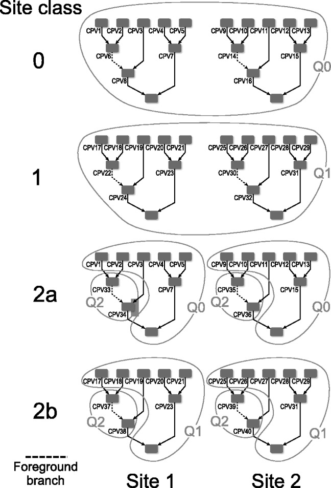
Analysis on how many elementary subtree computations are necessary in the branch-site model; CPVm correspond to m distinct conditional probability vectors, where matching m need to be computed only once; Q identify three distinct Q matrices for distinct values

2 IMPROVEMENTS

Here we discuss optimization techniques that we propose. Note that we have not added any heuristics, and each of the following improvements is supposed to be beneficial independent of the number of species and independent of the number of alignment sites. Specific implementation issues are described along with each optimization technique.

2.1 Sequential improvements

2.1.1 Subtrees reuse

The per-site likelihoods for a MSA are independent of each other and can thus be computed in an arbitrary order. If two or more sites of the MSA are identical, it suffices to only compute the logarithmic likelihood (lnL) on one site and multiply it by the number of identical sites to obtain the total lnL. This technique is used in most likelihood-based software, but there are further redundant computations caused by re-occurring patterns in the MSA.

In each subtree, there is a potential to economize CPV computations for different sites of the MSA. If the same state appears at two or more sites of a sequence, all occurrences yield identical CPVs at the particular leaf. If the patterns of the sub-alignment induced by a subtree match are identical for two or more sites, the corresponding CPVs for the two sites are also identical. However, identical patterns in the sub-alignments induced by a subtree need to be identified first. The identification of such identical patterns in sub-alignments can be done, e.g. by searching (i) sequentially or (ii) using a symbol table (Sedgewick and Wayne, 2011, p.361). In the latter case, the key is the index of the CPV within the tree, and the value associated with the key is its CPV. In the straightforward approach (i), there are no costs on storing values, but up to m – 1 lookups for a matching subpattern, where m is the length of the MSA. For huge MSAs, it may be advantageous to implement the second approach, where the additional cost for storing or linking site patterns is compensated by a faster lookup. In FastCodeML, we identify reusable subtree patterns in a preprocessing step and tag each node with the codon sequence identified by the subtree rooted in this node. Subsequently, a lookup of these tags for all sites with identical subtrees is done. Once identified, the CPV that can be re-used is linked via a pointer in the reusing tree, that is, this saves the costs of computing this particular CPV. The unused subtree can be freed to reduce memory consumption. In the example of Figure 2, computing the two CPVs incident to two leaves in box ① and the CPV at ② are redundant, because both codon sites feature an identical subtree: all involved CPVs match. Thus three CPV computations can be saved.

Fig. 2.

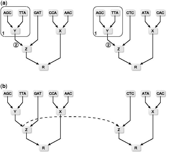
Subtrees reuse strategy depicted for two (not necessarily neighboring) sites in the MSA; in (a) subtree (1) contains identical codons for both sites; consequently, in (b) the CPVs for both sites are identical and need to be computed only once (dotted line)

Related techniques for extending pattern detection and re-use in the MSA to the subtree level have already been proposed (Izquierdo-Carrasco et al., 2011; Stamatakis et al., 2002; Sumner and Charleston, 2010). However, they focus on detecting patterns and avoiding redundant likelihood computations on trees whose topologies change in the course of ML tree search. For dynamically changing trees, a trade-off between the pattern detection and memory storage costs and the amount of saved computations needs to be achieved. To reduce the cost of pattern detection, the initial implementation of the Subtree Equality Vector (SEV) technique (Stamatakis et al., 2002) only considered subtree patterns that contained a single identical character. The book keeping was subsequently further simplified to sites consisting entirely of gaps (Izquierdo-Carrasco et al., 2011). In Kosakovsky Pond and Muse (2004), the authors suggest to sort nucleotide-based MSAs by site similarity to avoid redundant computations. This approach minimizes memory consumption, as only a subset of sites needs to be kept in memory. However, this incurs additional costs for rearranging the sites in order to maximize the number of lookups from neighboring sites. The memory consumption for our application scenario (Selectome database updates) does not represent a limiting factor. Hence, all CPVs can be kept in memory, avoiding the expensive reordering of sites. However, especially for memory-intensive approaches, it may be more effective to keep only a subset of all CPVs in memory and consider site sorting.

2.1.2 New matrix exponential and CPV computation

In Schabauer et al. (2012), we transformed the problem of computing the matrix exponential of non-symmetric Qt into a symmetric problem as follows: we define the symmetric matrix and compute its eigendecomposition . By introducing , the matrix exponential of Qt becomes .

An additional modification transforms the final asymmetric matrix–vector multiplication into a symmetric matrix–vector product:

(1)

(2)

Note that is by construction a symmetric matrix, whereas is generally asymmetric. The advantage of this modification is that the symmetry reduces the number of necessary matrix memory accesses by approx. 50% (Golub and Van Loan, 2013, p.18). This technique has been implemented in FastCodeML.

2.1.3 LRT optimization

When optimizing parameter values for H₀ and H₁ one after the other, one can save on parameter optimization steps. Each step in the parameter optimization procedure improves the associated lnL of the tree until convergence has been reached. In this discussion, the optimizer may modify all parameter values at each single step. One can either (i) optimize H₀ first with high accuracy and iteratively improve H₁ afterwards: once becomes larger than , the parameter optimization for H₁ can be stopped because the LRT is already significant. This potentially saves optimization steps for H₁. Or we can (ii) optimize H₁ first, then proceed analogously: the parameters of H₀ are optimized until becomes smaller than . In general, a significant LRT (i.e. detecting positive selection) is a relatively rare event (Kosiol et al., 2008; Studer et al., 2008). Strategy (i) saves optimization steps if positive selection occurs; strategy (ii) saves optimization steps if not. Consequently, without prior knowledge of the frequency of occurrence of positive selection in the MSA at hand, strategy (ii) (implemented in FastCodeML) will yield larger savings. If the LRT is significant, a BEB is applied to identify the sites under positive selection. Otherwise, FastCodeML does not execute the BEB, in contrast to CodeML. In the general case, this optimization is applicable if different models are compared, where each of them is optimized iteratively.

2.2 Parallelization

While the parallelization of ML-based nucleotide- protein- and codon models has already been addressed (Stamatakis, 2011) (e.g. RAxML, IQPNNI, HyPhy), it has mostly been in the context of tree topology optimization, and not for the likelihood itself. The main challenge in parallelizing ML-based phylogeny computations comes from the tree structure that leads to an irregular domain decomposition (Tomko, 1995). An efficient parallelization of the BSM is even more challenging due to its site classes and dependencies in between.

Our implementation optimizes simultaneously all the parameters. The maximizer acts as an impenetrable boundary for parallelization, and we distinguish parallelization ‘above’ (coarse-grain) and ‘within’ (fine-grain) this boundary (cf. supplementary material, Fig. 1).

2.2.1 Coarse-grain parallelization:

Gene-wise parallelization. Because distinct genes typically have different evolutionary histories with distinct branch lengths and evolutionary parameters, phylogenies for genes are commonly estimated independently for each gene. Consequently, single genes cannot be concatenated into multi-gene alignments to attain high scalability by means of a fine-grain parallelization of the likelihood function [see, e.g. (Stamatakis and Ott, 2009)]. Here we test for selection independently (gene-wise), these analyses can be carried out in an embarrassingly parallel way [see, e.g. (Foster, 1995, p.21)].

Foreground branch parallelization. A further BSM parallelization option is the simultaneous analysis of distinct foreground branches. This is possible because we want to test for positive selection on each branch of a given phylogeny. Thus, the tests for positive selection, where n is the number of taxa, can be conducted in parallel by duplicating the tree data structure and CPVs.

Under this parallelization strategy, a dedicated master process broadcasts all model parameters, tree topologies and branch lengths to all worker nodes. The workers then conduct the tests independently of each other on different foreground branches of the same tree. Afterwards, the worker nodes return the estimated parameter values and the lnL scores to the master process. We implemented this approach using MPI (Message Passing Interface Forum, 1994). The foreground-branch based parallelization can be combined with a site-wise fine-grain parallelization of the per-tree likelihood computations (Section 2.2.2) into a hybrid parallelization scheme.

Hypotheses parallelization. Note that for each foreground branch, hypotheses H₀ and H₁ can be computed independently and simultaneously, thus increasing the degree of parallelism. However, the simultaneous computation of H₀ and H₁ prevents us from using the aforementioned LRT optimization (Section 2.1.3). Although the LRT and the subsequent BEB must be computed after H₀ and H₁, they can be parallelized between different foreground branch computations. This parallelization strategy can be applied whenever two evolutionary models are compared. It is implemented in FastCodeML via the same master-worker scheme.

2.2.2 Fine-grain parallelization:

Site-wise parallelization. A common way to parallelize likelihood computations on shared memory architectures is by parallelizing over the sites of the MSA. This site-wise parallelization can be implemented using OpenMP or POSIX Threads. MPI-based implementations exist but focus on large MSAs that are outside the scope of this article. However, while our subtree patterns re-use scheme (Section 2.1.1) reduces the number of computations along the branches, it poses a load balance challenge: (i) a particular CPV for a site can only be computed after the site whose results it reuses (i.e. data dependency) has been computed and (ii) a site that reuses a previously computed CPV exhibits a smaller workload which leads to load imbalance.

The load balancing strategy we use in FastCodeML subdivides the alignment sites into groups such that each group exclusively reuses subtrees from the previous groups (Fig. 3). Each group is assigned a rank value starting from zero. CPVs from groups with lower rank values can potentially be reused. The first group does not reuse any subtree. All subtrees of a group can be parallelized, because they are independent of each other. The groups are then computed sequentially in order of rank. To balance the load for each group, subtrees can be moved to higher ranked groups. To increase parallelism, the trees of each group are replicated for each site class that should be computed until no lower rank group depends on it. The parallelization inside each group has been implemented using OpenMP.

Fig. 3.

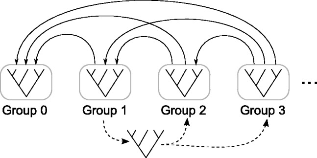
Load balancing strategy: the sites of the tree are grouped so that each group depends only on groups at its left (continuous lines). A tree can be moved to a group to its right (dashed line) only if it has no dependencies from other trees in intermediate groups

This site-wise parallelization strategy including load balancing can likewise be applied to nucleotide- or protein-based MSAs. The parallel performance may vary due to different computational load per site.

2.3 Implementation

FastCodeML has been implemented from scratch (except for the BEB that was largely taken from the CodeML codebase) in ISO C++ 2003 utilizing BLAS and LAPACK for linear algebra operations, and Spirit (http://www.boost.org/doc/libs/release/libs/spirit/) for tree parsing. We use the parameter optimization codebase of CodeML.

3 EVALUATION

We measure median runtimes of 10 individual runs for each evaluation (three on the large scale analysis in Section 3.5). Speedup values are determined by , where T₁ is the runtime (elapsed time, wall-clock time) of the reference execution and T₂ the runtime of the execution to be evaluated on the same dataset; for a relative speedup T₁ and T₂ denominate runtimes of the same executable, while for the absolute speedup T₁ is strictly the original CodeML. Initial branch lengths were read from file, while model parameters are initialized randomly. Memory consumption of CodeML, SlimCodeML and FastCodeML for these datasets is not a limiting factor and therefore not performance critical. Although a single executable can be used for all subsequent evaluations, we built sequential, OpenMP parallelized, MPI parallelized and hybrid executables separately. A summary of the platforms used can be found in the supplementary material.

3.1 Datasets

Table 1 contains the six datasets we used for evaluation. With respect to the Selectome database, these empirical datasets are representative for the cases: (D1) small number of species/medium sequence length; (D2) small number of species/large sequence length; (D3) medium number of species/small sequence length; (D4) large number of species/short sequence length; (D5) a simulated dataset with positive selection based on dataset D1 (using PAML’s evolver choosing ‘evolverNSbranchsites’ for the BSM with ). Finally, we analyse in D6 a very large rbcL dataset (Grass Phylogeny Working Group II, 2012) which cannot be processed in a feasible time by CodeML.

Table 1.

Test datasets of our analyses; remaining branches is the percentage of non-redundant branches for the given data over all sites of the alignment; dataset D5 is generated based on ENSGT00390000016702.Primates.1 with

Abbr.	Full name	No. of species	No. of branches	Remaining branches [%]	Length (codons)
D1	ENSGT00390000016702.Primates.1	7	12	37.74	299
D2	ENSGT00530000063518.Primates.1	95	188	75.49	39
D3	ENSGT00550000073950.Euteleostomi.7	25	48	56.31	67
D4	ENSGT00580000081590.Primates.1	6	10	20.92	5004
D5	Generated by evolver (PAML)	7	12	38.04	282
D6	Grass_rbcL	506	1242	19.54	414

3.2 Accuracy

In Table 2 we analyse the accuracy of FastCodeml with respect to lnLs and LRT scores. We use SlimCodeML as a proxy for good accuracy, as it gives very similar results as CodeML (Schabauer et al., 2012), which is the established gold standard. We note that the accuracy of computed lnLs is much higher than typically required to discriminate between significant and insignificant LRTs.

Table 2.

Accuracy of SlimCodeML and FastCodeml on Macpro; is the absolute difference of lnLs comparing either SlimCodeML or FastCodeML with CodeML on H₀ (H₁), respectively

	Dataset			LRT	pos. selection
SlimCode versus CodeML	D1				no (✓)
	D2				no (✓)
	D3				no (✓)
	D4				no (✓)
	D5			10.4	site 239 (✓)
FastCodeML versus CodeML	D1				no (✓)
	D2				no (✓)
	D3				no (✓)
	D4				no (✓)
	D5			10.4	site 239 (✓)

Note: ‘✓’ indicates agreement of the computed result with CodeML.

3.3 Sequential runtimes

Sequential speedups of FastCodeML (single-threaded) versus CodeML and SlimCodeML for five datasets (H₀ and H₁, respectively) on platform Macpro (cf. supplementary material) are depicted in Figure 4; here, FastCodeML includes the following improvements: faster matrix exponentiation (Section 2.1.2) and subtrees reuse (Section 2.1.1). LRT optimization (Section 2.1.3) is not considered, as either H₀ or H₁ is computed per run. We observe speedups of FastCodeML versus CodeML ranging from 2.6 to 5.8. The sequential FastCodeML is significantly faster than both CodeML and SlimCodeML on all five datasets.

Fig. 4.

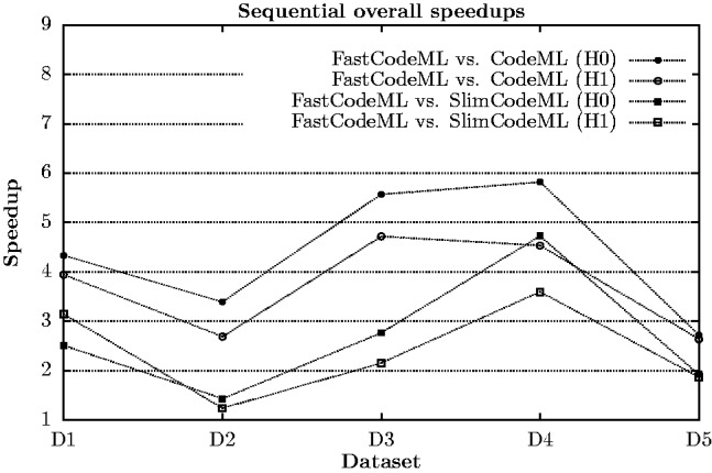
Sequential speedups of FastCodeML in comparison with CodeML and SlimCodeML on Macpro for H₀ and H₁, respectively

3.4 Parallel runtimes

3.4.1 Site-wise parallelization

Figure 5 shows the scaling of FastCodeML on a site-wise (OpenMP based) parallelization strategy for dataset D2 on 1–12 CPU cores (one thread per core); we observe relative speedups comparing FastCodeML in versus 1 threads, reaching 11.1 for 12 cores without subtrees reuse, and speedups up to 7.6 for 12 cores with subtrees reuse. These relative speedups correspond to absolute speedups versus CodeML of up to 23.4 without subtrees reuse, and speedups up to 19.9 with subtrees reuse. While scaling of subtrees reuse is slightly worse than without subtrees reuse, absolute runtimes on this particular platform and dataset suggest to enable subtrees reuse on 1–11 cores but not on 12. The worse scaling of subtrees reuse is presumably caused by load imbalance. Due to differences in the sequential performance of subtrees reuse, we also expect the performance of parallel subtrees reuse to vary with different datasets. In general, the effectiveness of parallel subtrees reuse is a trade-off between the number of redundant branches versus the data dependencies introduced.

Fig. 5.

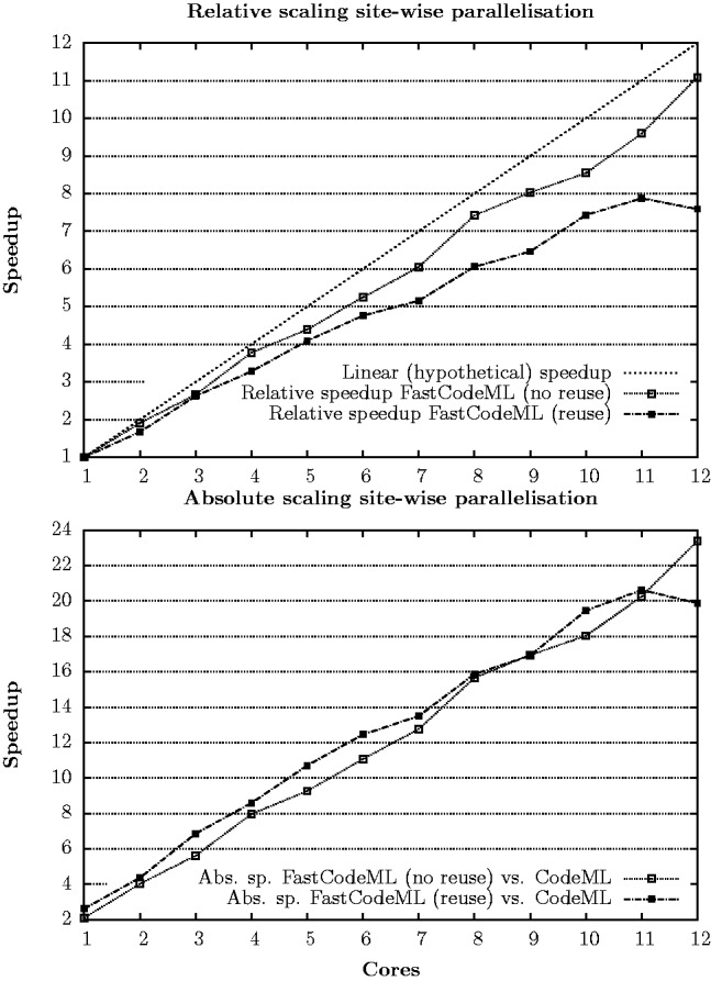
Parallel site-wise relative (top) and absolute (bottom) speedups of FastCodeML on Castor on dataset D2 for H₁

3.4.2 Foreground branch-based parallelization

Figure 6 depicts the relative scaling of FastCodeML on a foreground-branch based parallelization strategy. The evaluation has been done for dataset D3 on 1–7 worker nodes (single thread per node). Due to the master–worker scheme used, performance gains are observed for two or more worker nodes. The analysis is done for all possible 22 foreground branches, where the runtime for CodeML is measured only on a single foreground branch but multiplied by 22; running CodeML on all foreground branches is expected to consume more than a day. We observe relative speedups of up to 5.9 on 7 worker nodes, which corresponds to absolute speedups from 3.3 to 19.4. In general, the relative speedup for foreground branch-based parallelizations benefits from a high ratio of foreground branches to available nodes, as the workload can more easily be divided into balanced parts.

Fig. 6.

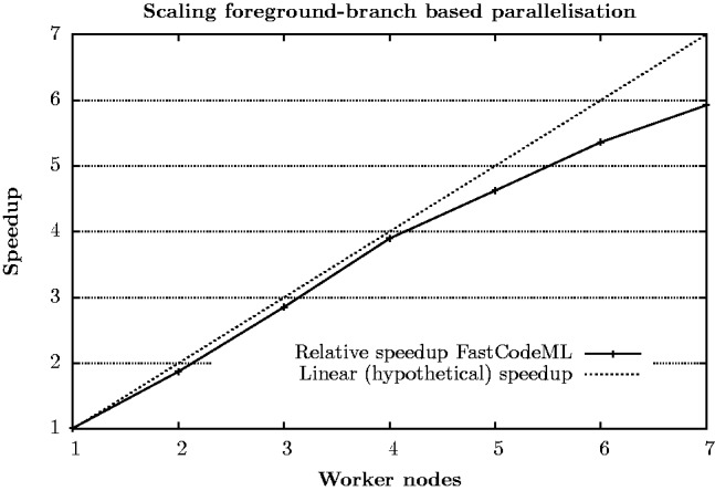
Parallel foreground branch (MPI based) relative speedups of FastCodeML for dataset D3 on Castor for H₁; only a single CPU core per node was used

3.4.3 Hybrid parallelization

Figure 7 depicts absolute scaling of FastCodeML on a hybrid (foreground branch and site-wise) parallelization strategy implemented using OpenMP and MPI on 1–7 worker nodes, where all 12 CPU cores are used. Corresponding runtimes, relative and absolute speedup values are summarized in Table 3. We observe relative speedups up to 6.3 on 7 worker nodes, which corresponds to absolute speedups up to 170.9.

Fig. 7.

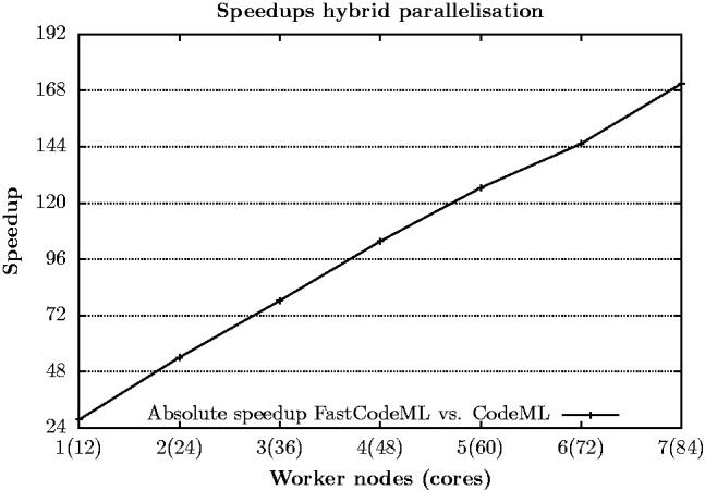
Parallel hybrid (OpenMP and MPI based) scaling of FastCodeML for dataset D3 on Castor for H₁

Table 3.

Overall parallel performance of FastCodeml versus CodeML on Castor for dataset D3 on all possible foreground branches for H₁; CodeML runtime for absolute speedups is extrapolated from computing a single foreground branch

Worker nodes (cores)	FastCodeML runtime [s]	Rel. speedup	Abs. speedup
1 (12)	429	1	27.6
2 (24)	218	2	54.2
3 (36)	151	2.9	78.4
4 (48)	114	3.8	103.7
5 (60)	93	4.7	126.5
6 (72)	81	5.4	145.3
7 (84)	69	6.3	170.9

3.5 Large scale analysis

A large scale analysis has been conducted to prove the use of FastCodeML beyond the capabilities of CodeML. In initial tests, we verified that dataset D6 achieves its best runtime performance on platform Castor (cf. supplementary material) by using all 12 available cores per node and by reusing subtrees (Section 2.1.1). We analysed D6 for H₀ and H₁ running FastCodeML (multi-threading) on 12 CPU cores and determined average runtimes of three test runs. The average runtime of FastCodeML on dataset D6 is 21.9 h for H₀ and 31.9 h for H₁. Due to time restrictions, we evaluated only a single iteration of CodeML for D6 which took 2.2 h on H₀ (367 iteration steps) and 2.3 h on H₁ (426 iteration steps) on the same platform. As we apply the same parameter optimization codes, we use the average number of optimization steps of FastCodeML on dataset D6 for the following speedup metric: we extrapolate that CodeML would have finished executing in approximately h (i.e. ca. 33.6 days) for H₀ and h (i.e. ca. 40.8 days) for H₁. The estimated speedups comparing the single threaded CodeML with FastCodeML running in 12 threads is thus 36.9 for H₀ and 30.7 for H₁. In this example, the LRT optimization saves 268 optimization steps for H₁ (63%).

4 CONCLUSIONS

We introduced here three sequential code optimizations: an improved matrix exponential, subtrees reuse and LRT optimization. We observed significant speedups versus both CodeML and our previous version SlimCodeML, and the first two optimizations can be used in various likelihood computations in phylogenetics. Moreover, we present a parallelization strategy that uses a fine-grain and a coarse-grain approach. Overall, our improvements allow for testing selection on phylogenetic trees which exceed the possibilities of the original CodeML software; this is crucial to tackle the genomic data avalanche. The discussed improvements are motivated by the branch-site model but can, due to the likelihood framework, be extended to nucleotide- and amino acid-based MSAs as well as Bayesian approaches. We briefly identified such opportunities where applicable, but an extensive discussion is subject to future work.

The optimization of the likelihood surface for phylogenetics problems is complex and we have started experimenting with the alternative parameter optimizers available in NLopt (http://ab-initio.mit.edu/wiki/index.php/NLopt). It may be interesting to compare different implementations of the Broyden–Fletcher–Goldfard–Shanno (BFGS) optimization method, but a deeper investigation of the global and derivative-free optimizers is needed to better understand the potential solutions to find the maximum likelihood estimator for complex evolutionary models.

In a future version the dependencies between nodes could be modelled as a directed acyclic graph and the parallelism be based on a dataflow model (YarKhan et al., 2011) to study and potentially further improve parallel performance. Moreover, the site classes could be included into the dependency graph. This way a more fine-grained parallelism could be achieved. Increasing the parallel performance becomes crucial with the trend of more parallelism in future computer platforms (Dongarra, 2012).

REFERENCES

- Anisimova M, Kosiol C. Investigating protein-coding sequence evolution with probabilistic codon substitution models. Mol. Biol. Evol. 2009;26:255–271. doi: 10.1093/molbev/msn232. [DOI] [PubMed] [Google Scholar]
- Anisimova A, Yang Z. Multiple hypothesis testing to detect lineages under positive selection that affects only a few sites. Mol. Biol. Evol. 2007;24:1219–1228. doi: 10.1093/molbev/msm042. [DOI] [PubMed] [Google Scholar]
- Bai Z, et al. Templates for the Solution of Algebraic Eigenvalue Problems: A Practical Guide. Philadelphia: SIAM; 2000. [Google Scholar]
- Comnish-Bowden A. Nomenclature for incompletely specified bases in nucleic acid sequences: recommendation 1984. Nucleic Acids Res. 1985;13:3021–3030. doi: 10.1093/nar/13.9.3021. [DOI] [PMC free article] [PubMed] [Google Scholar]
- Dongarra JJ. High performance computing systems: status and outlook. Acta Numerica. 2012;21:379–474. [Google Scholar]
- Dutheil JY, et al. Efficient selection of branch-specific models of sequence evolution. Mol. Biol. Evol. 2012;29:1861–1874. doi: 10.1093/molbev/mss059. [DOI] [PubMed] [Google Scholar]
- Felsenstein J. Evolutionary trees from DNA sequences: a maximum likelihood approach. J. Mol. Evol. 1981;17:368–376. doi: 10.1007/BF01734359. [DOI] [PubMed] [Google Scholar]
- Foster IT. Designing and Building Parallel Programs. Reading, Mass: Addison-Wesley; 1995. [Google Scholar]
- Gil M, et al. CodonPhyML: fast maximum likelihood phylogeny estimation under codon substitution models. Mol. Biol. Evol. 2013;30:1270–1280. doi: 10.1093/molbev/mst034. [DOI] [PMC free article] [PubMed] [Google Scholar]
- Golub GH, Van Loan CF. Matrix Computations. 4th edn. Baltimore, MD: Johns Hopkins University Press; 2013. [Google Scholar]
- Grass Phylogeny Working Group II. New grass phylogeny resolves deep evolutionary relationships and discovers C4 origins. New Phytol. 2012;193:304–312. doi: 10.1111/j.1469-8137.2011.03972.x. [DOI] [PubMed] [Google Scholar]
- Izquierdo-Carrasco F, et al. Algorithms, data structures, and numerics for likelihood-based phylogenetic inference of huge trees. BMC Bioinformatics. 2011;12:1–14. doi: 10.1186/1471-2105-12-470. [DOI] [PMC free article] [PubMed] [Google Scholar]
- Kosakovsky Pond SL, Muse SV. Column sorting: rapid calculation of the phylogenetic likelihood function. Syst. Biol. 2004;53:685–692. doi: 10.1080/10635150490522269. [DOI] [PubMed] [Google Scholar]
- Kosiol C, et al. Patterns of positive selection in six mammalian genomes. PLoS Genet. 2008;4:e1000144. doi: 10.1371/journal.pgen.1000144. [DOI] [PMC free article] [PubMed] [Google Scholar]
- Kraut A, et al. HealthGrid. Birmingham, AL: IOS Press; 2010. Phylogenetic code in the cloud – can it meet the expectations? pp. 55–63. [PubMed] [Google Scholar]
- Lartillot N, Philippe H. A bayesian mixture model for across-site heterogeneities in the amino-acid replacement process. Mol. Biol. Evol. 2004;21:1095–1109. doi: 10.1093/molbev/msh112. [DOI] [PubMed] [Google Scholar]
- Lemey P, et al. A counting renaissance: combining stochastic mapping and empirical Bayes to quickly detect amino acid sites under positive selection. Bioinformatics. 2012;28:3248–3256. doi: 10.1093/bioinformatics/bts580. [DOI] [PMC free article] [PubMed] [Google Scholar]
- Message Passing Interface Forum. MPI: a message-passing interface standard. Int. J. Supercomput. Appl. High Performance Comput. 1994;8:3–4. [Google Scholar]
- Murrell B, et al. Detecting individual sites subject to episodic diversifying selection. PloS Genet. 2012;8:e1002764. doi: 10.1371/journal.pgen.1002764. [DOI] [PMC free article] [PubMed] [Google Scholar]
- Nielsen R. Statistical Methods in Molecular Evolution. New York: Springer; 2005. [Google Scholar]
- Proux E, et al. Selectome: a database of positive selection. Nucleic Acids Res. 2009;37:404–407. doi: 10.1093/nar/gkn768. [DOI] [PMC free article] [PubMed] [Google Scholar]
- Rannala B, Yang Z. Phylogenetic inference using whole genomes. Annu. Rev. Genomics Hum. Genet. 2008;9:217–231. doi: 10.1146/annurev.genom.9.081307.164407. [DOI] [PubMed] [Google Scholar]
- Rodrigue N, Aris-Brosou S. Fast bayesian choice of phylogenetic models: prospecting data augmentation-based thermodynamic integration. Syst. Biol. 2011;60:881–887. doi: 10.1093/sysbio/syr065. [DOI] [PubMed] [Google Scholar]
- Schabauer H, et al. 11th International Workshop on High Performance Computational Biology (HiCOMB) New York: IEEE; 2012. SlimCodeML: an optimized version of CodeML for the branch-site model; pp. 700–708. [Google Scholar]
- Sedgewick R, Wayne K. Algorithms. 4th edn. Reading, Mass: Addison-Wesley; 2011. [Google Scholar]
- Seo TK, Kishino H. Synonymous substitutions substantially improve evolutionary inference from highly diverged proteins. Syst. Biol. 2008;57:367–377. doi: 10.1080/10635150802158670. [DOI] [PubMed] [Google Scholar]
- Stamatakis A. Orchestrating the phylogenetic likelihood function on emerging parallel architectures. In: Schmidt B, editor. Bioinformatics—High Performance Parallel Computer Architectures. Singapore: CRC Press; 2011. pp. 85–115. [Google Scholar]
- Stamatakis A, Ott M. ICPP. New York: IEEE; 2009. Load balance in the phylogenetic likelihood kernel; pp. 348–355. [Google Scholar]
- Stamatakis A, et al. Bioinformatics Conference. New York: IEEE; 2002. AxML: a fast program for sequential and parallel phylogenetic tree calculations based on the maximum likelihood method; pp. 21–28. [PubMed] [Google Scholar]
- Studer RA, et al. Pervasive positive selection on duplicated and nonduplicated vertebrate protein coding genes. Genome Res. 2008;18:1393–1402. doi: 10.1101/gr.076992.108. [DOI] [PMC free article] [PubMed] [Google Scholar]
- Sumner J, Charleston M. Phylogenetic estimation with partial likelihood tensors. J. Theor. Biol. 2010;262:413–424. doi: 10.1016/j.jtbi.2009.09.037. [DOI] [PubMed] [Google Scholar]
- Tomko KA. Domain Decomposition, Irregular Applications, and Parallel Computers. 1995. Ph.D. thesis, University of Michigan, Michigan. [Google Scholar]
- Venditti C, et al. Phylogenetic mixture models can reduce node-density artifacts. Syst. Biol. 2008;57:286–293. doi: 10.1080/10635150802044045. [DOI] [PubMed] [Google Scholar]
- Yang Z. Computational Molecular Evolution. Oxford: Oxford University Press; 2006. [Google Scholar]
- Yang Z, et al. Bayes empirical bayes inference of amino acid sites under positive selection. Mol. Biol. Evol. 2005;22:1107–1118. doi: 10.1093/molbev/msi097. [DOI] [PubMed] [Google Scholar]
- YarKhan A, et al. QUARK Users’ Guide: QUeueing and Runtime for Kernels. 2011. Technical report. University of Tennessee Innovative Computing Laboratory. ICL-UT-11-02, Tennessee. [Google Scholar]
- Zhang J, et al. Evaluation of an improved branch-site likelihood method for detecting positive selection at the molecular level. Mol. Biol. Evol. 2005;22:2472–2479. doi: 10.1093/molbev/msi237. [DOI] [PubMed] [Google Scholar]
Associated Data
This section collects any data citations, data availability statements, or supplementary materials included in this article.