Evolutionary dynamics of n-player games played by relatives

Abstract

One of the core concepts in social evolution theory is kin selection. Kin selection provides a perspective to understand how natural selection operates when genetically similar individuals are likely to interact. A family-structured population is an excellent example of this, where relatives are engaged in social interactions. Consequences of such social interactions are often described in game-theoretical frameworks, but there is a growing consensus that a naive inclusive fitness accounting with dyadic relatedness coefficients are of limited use when non-additive fitness effects are essential in those situations. Here, I provide a general framework to analyse multiplayer interactions among relatives. Two important results follow from my analysis. First, it is generally necessary to know the n-tuple genetic association of family members when n individuals are engaged in social interactions. However, as a second result, I found that, for a special class of games, we need only measures of lower-order genetic association to fully describe its evolutionary dynamics. I introduce the concept of degree of the game and show how this degree is related to the degree of genetic association.

1. Introduction

Kin selection theory describes evolutionary consequences of social interactions that occur between individuals, especially between those who are genetically or phenotypically correlated such as relatives [1–8]. One of its major contributions to evolutionary biology is that the theory revealed the possibility of evolution of self-sacrificing cooperation towards kin [9–16]. In the simplest case, this fact is beautifully demonstrated by an inclusive fitness accounting, namely that such a cooperation evolves if the benefit of cooperation weighted by the relatedness to the beneficiary exceeds its cost, famously known as Hamilton's rule [1,17,18].

Game theory, on the other hand, often presupposes a more complex type of interaction than a simple unilateral donation of cooperation [19–21]. The virtue of game theory lies in that it can describe social interactions where one's pay-off not only depends on your own action but also, often non-additively, on partners' ones. For example, in the traditional hawk–dove game, the advantage of choosing an aggressive strategy, hawk, very much depends on the strategy of the co-player; the outcome of a hawk–hawk interaction is detrimental owing to the fighting cost, whereas the outcome of a hawk–dove interaction is the most profitable for the hawk player, because he wins all the resources [22,23].

Therefore, an evolutionary consequence of game interactions between relatives is not obvious [24–27]. There is a large amount of literature indicating that a simple inclusive-fitness accounting as provided by Hamilton [1] does not always work for complex interactions [2,3,10,20,25,28–40] (but see [7]), and it has been shown that this is especially true when we study games with discrete strategies (i.e. pure hawk or pure dove) rather than with continuous ones (i.e. mixed strategies of hawk and dove) [41–43]. Some literature suggests that higher-order genetic association of more than two individuals is necessary to fully describe evolutionary game dynamics [15,30,31,44–48].

Despite analytical difficulty, social interaction among kin is ubiquitous in biology. Recent developments in microbiology revealed that microbes are engaged in various kinds of social interactions [49–57]. An essential feature is that those microbes often clonally reproduce and therefore they are inevitably genetically highly related to each other. The reason for such an assortment is mainly due to spatial structure and limited dispersal [58,59]. As another instance, in larger animals such as primates, we often find nepotistic cooperation among kin [60–62].

A goal of this paper was to clarify the evolutionary game dynamics when players are related to each other. A milestone work in this direction is that of Grafen [25], who studied a hawk–dove game played between two relatives. However, real social interactions do not necessarily involve only two individuals. As seen from examples above, in many situations, more than two relatives are simultaneously involved in a single social interaction. This motivates me to extend an existing two-player game model to an n-player one to see its evolutionary game dynamics.

2. Model

I assume an infinitely large population of haploid individuals. Each individual adopts one of the two strategies, A or B, that are genetically determined and genetically inherited from a parent. I can phrase these assumptions in terms of cultural evolution; in this case, one's strategy is culturally transmitted.

At each time step, groups of n-players are formed in order for them to play an n-player game. The pay-off of an A-player when k (0 ≤ k ≤ n − 1) of the other n − 1 players in the group choose A (and therefore n − 1 − k other players choose B) is denoted by a_k. Similarly, the pay-off of a B-player when k (0 ≤ k ≤ n − 1) of the other n − 1 players in the group choose A is given by b_k. In other words, a list of and defines a single game.

The most important assumption of my model is that the formation of groups of n-individuals is not random but assortative, often favouring kin (i.e. nepotistic). This means, for example, that relatives are more likely to come together than expected by chance. I do not explicitly specify an actual process of assortative group formation, but for later use in my analysis I need to know the average property of such groups with respect to common ancestry. More specifically, imagine infinitely many groups of n-individuals that are formed through a certain process of assortative grouping. Then, randomly take ℓ (1 ≤ ℓ ≤ n) different individuals from a randomly sampled group and ask who shares a common ancestor with whom. Let θ_{ℓ →m} be the probability that those ℓ different individuals have m (1 ≤ m ≤ ℓ) different origins in an ancestral population (theoretically speaking, infinitely) many generations before. One trivial case is m = 1, which means that all the ℓ individuals share a single common ancestor. Another trivial case is m = ℓ, where no two individuals share a common ancestor. Because I do not assume any mutations in strategy during reproduction, players sharing a common ancestor always share the same strategy. Therefore, the probabilities θ_{ℓ →m} (1 ≤ m ≤ ℓ ≤ n) measure the extent of genetic association in the group of n individuals.

After group formation, those n-players in the same group are involved in the n-player game described above, and each player gains an individual pay-off, f. This pay-off is translated into its fecundity, 1 + δf, where one is the baseline value and δ can be any positive constant as long as everyone's fecundity is guaranteed to be strictly positive. Then, each player produces multiple gametes in proportion to their fecundity, and the next generation is formed by either asexual or sexual reproduction. In the case of asexual reproduction, gametes directly grow into adults. For sexual reproduction, two (or possibly more) gametes are chosen randomly, they fuse, and all but one gamete instantly vanish to make haploid individuals in the next generation. Generations can be either non-overlapping or overlapping. I assume that a fraction, s, of adult individuals in the previous generation survive and that newborns compete on an equal basis for the vacancies that arise owing to the death of adults in the previous generation. Quite importantly, I assume that such a competition among newborns occurs globally, so no local regulation of the population is assumed. This assumption is critical for my results, especially the one in §5, which I will discuss later. It will soon be shown that the parameter s does not affect the results qualitatively.

Of central importance is to see how the overall frequency of A-strategists in the population, which is denoted by p in my paper, changes over time. To see this, I use a relative, not absolute, indexing of players in the population. More specifically, to any given focal player, I give the index 0, and to his n − 1 group members, I give indices of 1, 2, … , n−1, respectively. To conveniently express the strategies of those players, I introduce an indicator variable, p_i (0 ≤ i ≤ n − 1), that takes a value of either 1 or 0; if player i adopts strategy A, then its indicator variable is p_i = 1, and if B, then its value is p_i = 0.

(a). Calculation of pay-offs

Here, I calculate the game pay-off of a focal player. For that purpose, for 0 ≤ k ≤ n − 1, an indicator variable, ϕ_k, is defined. This new variable ϕ_k is equal to one if the number of A-strategists among its n − 1 group members is exactly equal to k, and otherwise zero. For example, ϕ_{n −1} can be easily constructed as (the product of p₁ to p_{n −1}), suggesting that all n−1 group members of the focal player adopt strategy A if and only if . In appendix A, I show that each ϕ_k (0 ≤ k ≤ n − 1) is expressed as a polynomial of .

With the help of ϕ_k, the game pay-off of a focal player is given by

2.1

That is, the focal player gains the pay-off of a_k if and only if p₀ = 1 (player adopts strategy A) and ϕ_k = 1 (exactly k other players adopt strategy A). Similarly, the focal player gains the pay-off of b_k if and only if 1 − p₀ = 1 (player adopts strategy B) and ϕ_k = 1 (exactly k other players adopt strategy A).

(b). Evolutionary dynamics

The change in the frequency of A-strategists in the population is described by the Price equation [63]

2.2

Here, w₀ is the expected fitness of a focal individual, defined as the probability of the focal individual surviving a single generation plus the expected number of his offspring that successfully replaced adults in the previous generation. w represents the average fitness in the population. The covariance above is defined by a hypothetical sampling of a focal player from the population [47,64]; in such a hypothetical sampling, randomness arises in whom I sample as a focal individual, so the indicator variable and the fitness of a focal individual can be regarded as random variables (and therefore this covariance is conditional on a given state of the population).

From my life cycle assumptions, the fitness of a focal player is given as

2.3

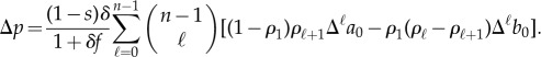
where f represents the average pay-off in the whole population. Combining equations (2.1)–(2.3), I arrive at the main result (see appendix A for its detailed derivation)

2.4

where ρ_ℓ (1 ≤ ℓ ≤ n) is the probability with which all different ℓ players who are randomly sampled from a randomly sampled group of n-players adopt strategy A (I set ρ₀ = 1). Remember that the probability with which those ℓ different players have m different origins is given by θ_{ℓ →m}. In such a case, I assume that those m different ancestral lineages are independent, and therefore that the probability with which all of those m lineages adopted strategy A in their ancestral state is given by p^m. Therefore, I obtain

2.5

Hereafter, I call ρ_ℓ ‘genetic association of degree ℓ’ or ‘ℓ-tuple genetic association’, because it measures genetic similarity of ℓ different individuals.

Two trivial cases are useful in facilitating our understanding of the main result, equation (2.4). The first baseline case lacks any genetic association, where we assume that ℓ different players always have ℓ different origins, so ρ_ℓ = p^ℓ follows. Substituting this in equation (2.4) gives us

2.6

where f_A and f_B are average pay-offs of an A-player and a B-player calculated based on a binomial sampling as

2.7

[65] (see appendix B for the derivation). The second case assumes that all n individuals in a group are clonal, leading to ρ₀ = 1 and ρ_ℓ = p for ℓ ≥ 1. In this case, equation (2.4) becomes

2.8

(see appendix B for the derivation), which makes sense because an A-player always interacts with n−1 A-players (pay-off = a_{n −1}), whereas a B-player always interacts with n−1 B-players (pay-off = b₀).

3. Two-player games

The case of n = 2 goes back to the analysis of two-player games between relatives by Grafen [25]. He assumed that the average relatedness between two-game players was given by r. In my terminology, this r corresponds to the probability with which a randomly sampled pair of players engaged in the two-player game shares a common ancestor. Therefore, θs of these two players are given by

3.1

leading to

3.2

[36,66]. Note that the second expression in equation (3.2) is the regression definition of relatedness given in Hamilton [66]. Grafen [25] studied a general two-strategy game where the pay-offs of A matched with A, A matched with B, B matched with A and B matched with B were respectively given by a, b, c, d. In my terminology, it corresponds to (a₀, a₁, b₀, b₁) = (b, a, d, c). Applying equation (2.4) to this specific example leads to

3.3

which correctly predicts the position of equilibrium described in eqn (6) in Grafen [25].

4. Three-player games

(a). Linear public goods game

Imagine a public goods game with three players, where strategy A corresponds to cooperation and B to defection. A cooperator pays the cost of C to contribute to the public goods, whereas a defector pays nothing. I assume that the net benefit of cooperation is given by B times the total number of cooperators, which is, in turn, equally divided by three players, irrespective of their contribution. This game is called a linear public goods game [67]. The pay-off of this game is given by

4.1

Applying equation (2.4) to the game (equation (4.1)) leads to

4.2

Observe that the triplet association, ρ₃, is absent from equation (4.2) but the dyadic association, ρ₂, is present. Substituting θs in equation (3.1) gives us

4.3

Note that the expression inside the square brackets in equation (4.3) can be understood intuitively in terms of inclusive fitness, that is, the benefit others received can be interpreted as if the focal player received that benefit, only after it is weighted by the genetic relatedness to those others. An interpretation is as follows. If I cooperate, I pay C but that increases the net benefit of public goods by B, benefiting each of the three individuals in the group by B/3. My relatedness to self is 1, and my relatedness to each of the other two is r, so the benefit B/3 should be weighted by 1 + 2r.

(b). Volunteer's dilemma

Here, I consider another three-player game. Similar to the previous example, strategies A and B correspond to cooperation and defection, respectively. A cooperator pays the cost, C, whereas a defector pays nothing. The difference between the public goods game and this game is that the benefit of cooperation, 3B, arises if and only if all the three players cooperate; in that case this benefit is equally distributed. Let me call this game the volunteer's dilemma after Archetti et al. [67] (see also [68]). The pay-off matrix of this game is given by

4.4

Setting C = 1 and B = 2, leads to the game analysed in Gardner et al. and van Veelen [7,28]. Applying equation (2.4) to this game leads to

4.5

The condition for evolution of cooperation is, therefore,

4.6

which reproduces the result of van Veelen [28, p. 597] and also reproduces eqn (14) in Gardner et al. [7]. The condition (4.6) explicitly contains the triplet association, ρ₃. Therefore, I need to specify the probabilities of three different players having m (1 ≤ m ≤ 3) origins, namely θ_{3 → m}, to derive its evolutionary dynamics.

Suppose that the probability θ_{2 →1} (relatedness) is r and that θ_{3 →1} (called triplet relatedness by Ohtsuki [30]) is s. These two probabilities measure the chance that two (or three) individuals share a unique common ancestor. In this case, I have

4.7

because there is a trivial relationship between θs (see appendix C). Then, the condition (4.6) is rewritten as

4.8

To see how (4.8) reveals the condition for evolution of cooperation between relatives, consider sexual reproduction and imagine that three full-sibs are engaged in the volunteer's dilemma, equation (4.4). It is easy to see that the coalescent probabilities of them are given by r = 1/2 and s = 1/4. Therefore, condition (4.8) becomes

4.9

On the other hand, if I consider three half-sibs who share a mother but never share a father, then I have r = 1/4 and s = 1/8, arriving at

4.10

Most importantly, a naive heuristics does not work here: that the left-hand side of (4.10) should be a half of the left-hand side of (4.9), because half-sibs are half as related as full-sibs. Rather, we observe that those left-hand sides are qualitatively different because they show different dependence on p.

5. Relationship between the degree of the game and degree of genetic association

One might wonder why ρ₃ is absent from the evolutionary dynamics of the linear public goods game, equation (4.1), but is present in its counterpart of the volunteer's dilemma game, equation (4.4), although both are three-player games. The answer lies in the nature of these games. As we can guess from its name, the pay-offs of the linear public goods game, equation (4.1), can be described by linear functions of k, as

5.1

By contrast, the pay-offs of the volunteer's dilemma, equation (4.4), can never be described by linear functions, but I need a quadratic function, as

5.2

For a general n-player game, the pay-offs, , can be described uniquely by a polynomial of k of degree n − 1 or smaller, so can be the pay-offs, . The largest degree of those two polynomials I shall define as the degree of the game. For example, both polynomials in equation (5.1) are of degree one, so the degree of the linear public goods game, equation (4.1), is 1. By contrast, those polynomials in equation (5.2) are of degree two and zero, respectively, so the degree of the volunteer's dilemma game, equation (4.4), is 2. The minimal and maximal degrees of n-player games are 0 and n − 1, respectively. Hereafter, I occasionally use the term ‘linear game’ to mean a degree-1 game.

In appendix D, I have proved that evolutionary dynamics of an n-player game of degree d can be described with genetic association of degree up to d + 1; in other words, ρ_{d + 1} is necessary to describe evolutionary game dynamics but higher ones such as are not. In short, the degree of nonlinearity of a game determines how high a genetic association is needed.

It is worth clarifying the difference between a degree-1 game and an ‘additive game’ [30], also known as a game of ‘(generalized) equal gains from switching’ [28]. Additivity is a useful concept in classifying social interactions, and the effect of deviation from additivity has been studied in some previous literature [30,67]. For my n-player, two-strategy game framework, additivity is defined in the following way. First, if the focal player adopts strategy A (or B), we think that it contributes to his pay-off by α₀ (or β₀). Second, if a player other than the focal player adopts strategy A (or B), we think that it contributes to the pay-off of the focal player by α (or β). Additivity means that the pay-off of the focal player is given by the sum of those contributions from the focal player and from the n − 1 other players. In this case, the pay-off is written as

5.3a

or

5.3b

Therefore, an additive game is a degree-1 game (except for the case of α = β) with the special property that the slopes of a_k and b_k (as linear functions of k) are the same.

A good example of an additive degree-1 game is the linear public goods game, equation (4.1). By contrast, a good example of a non-additive degree-1 game is the prisoner's dilemma game with synergism [20,30,37,43,47,69–71], given as

5.4

where strategies A and B represent cooperation and defection, respectively. The pay-offs B and C, respectively, represent the benefit and the cost of cooperation, and the pay-off D represents the synergistic effect of mutual cooperation.

6. Conclusion

In this paper, I have derived evolutionary game dynamics when family members of size n are engaged in a social interaction. The genetic structure of those family members is described by probabilities θ_{ℓ →m}, which tell us the chance that ℓ different individuals have m different origins. In other words, we need to know the coalescent tree structure of those individuals. Genetic association between two individuals is often measured by a relatedness coefficient, but I have shown that such dyadic relationship is, generally speaking, not sufficient to exactly tell the resulting evolutionary dynamics. To see why, imagine a task that can be completed only by full cooperation of all n members in the group. In such a case, the chance of success is equal to the chance of everyone being a cooperator, and therefore the probability with which those n individuals are simultaneously cooperators, namely n-tuple genetic association, is important. As one can see in this example, the pay-off in a multiplayer game is usually determined by joint effects of one's strategy and others' strategies. That is an intuitive reason of why higher-order genetic association is important. By contrast, for two-players games, one's pay-off is determined by one's own strategy and the partner's strategy, so a dyadic genetic association is enough to describe the evolutionary dynamics unless local competition is assumed (see eqn (15) in Lehmann & Keller [43] for example, and see also the discussion below).

It is not trivial to describe the kin structure of groups of more than two individuals. For example, McElreath & Boyd [72, p. 162] describe an n-player kin-biased group formation, assuming that the probability with which a colleague of an A-player adopting the same strategy is r + (1 − r)p, and that the probability with which two colleagues of an A-player simultaneously adopting strategy A is its square, [r + (1 − r)p]². However, the latter argument is generally wrong, because the conditional probability with which the second colleague adopting strategy A, given that both the first colleague and the focal individual adopt strategy A, is not equal to r + (1 − r)p if we take triplet genetic association into account.

One might wonder why I have not taken a more straightforward way to derive the evolutionary dynamics than considering genetic association, θ. In fact, van Veelen [69] provided a general machinery to analyse the n-player, two-strategy games studied here. He explicitly considered distribution of groups that differ in the number of A-players. Let us denote by q_k the frequency of groups with exactly k many A-players and (n − k) many B-players. In that case, the evolutionary dynamics, equation (2.4), is expressed in terms of q_k (0 ≤ k ≤ n). However, it is not obvious how measures of genetic association are mapped to those frequencies, q. Therefore, I have given a different expression of the same evolutionary dynamics in terms of genetic association to facilitate applications to family–group interactions. In studying interactions of three full-sibs, for example, it is much easier to specify their genetic association (r = 1/2 and s = 1/4, as in §4) than to explicitly calculate the frequencies of different groups, (q₀, q₁, q₂, q₃).

I have not explicitly modelled how assortative group formation favouring kin is done, in order to make the scope of application of my result as wide as possible. One of the mechanisms of such assortment is via kin recognition [45,46,73], where individuals discriminate others by using genetic or phenotypic markers. Understanding the interplay between social interaction and kin recognition is important, and extending the current model in such a direction should further enrich our understanding of social evolution based on nepotism.

Another plausible mechanism of assortative group formation is population viscosity often via limited dispersal [58,59,74–76]. Wright's island model [77] and its variants are typical ones in population genetics [30,44,45,78,79], and others prefer network formulations [80–82]. In any case, limited dispersal causes endogenous clustering of individuals with a common ancestry, thus those relatives are likely to interact. However, in these models, the effect of kin competition is not negligible, because limited dispersal hinders the transport of genes to the global gene pool, thus relatives must compete with each other over reproduction [38,75]. Such an effect is not incorporated in the fitness function, equation (2.3), because I have assumed global competition. Peña et al. recently studied n-player games in Wright's island model (J. Peña 2014, personal communication), which incorporate not only the primary effect of social interaction on evolutionary dynamics but also its secondary effect realized as local kin competition in demes.

The concept of degree of games introduced in my paper will be very useful to elucidate the connection between nonlinearity of games and degree of genetic association involved in the evolutionary dynamics. The reason why, in some cases, dyadic genetic relatedness, r, is sufficient for describing evolutionary dynamics is now clear, because the game is of degree one (i.e. the pay-offs a_k and b_k are linear in k). However, the main result in §5 that connects a game of degree d and genetic association of degree d + 1 strongly depends on the specific assumption of my model that population regulation occurs only globally. In other words, my model focuses on the primary effect of social interaction on the fecundity of interactants themselves, but not on the secondary effect that neighbours of those interactants receive. If one assumes the presence of local competition, such as in the Wright's island model or in network models, then a game of degree d would require higher genetic association than degree d + 1 for its evolutionary dynamics to be fully described. An example is given in Nowak et al. [29], which finds that evolutionary game dynamics of a non-additive two-player game (its degree is d = 1 except for degenerated cases) played in the Wright's island model needs not only dyadic genetic association (order 2) but also triplet genetic association (order 3) for its full description.

Although higher-order genetic association is important, there exists an exception where dyadic genetic association (dyadic relatedness, r) is enough to fully describe evolution; that is, when continuous strategies (i.e. mixed strategies) rather than discrete ones are discussed. In this case, an evolvable trait can be the probability of using strategy A, which ranges from zero to one. Studying the evolution of continuous strategies in n-player games is another direction of future study.

Appendix A. Deriving the main result

First, I write down ϕ_k in terms of . The following expression equals one, if and only if the number of A-strategists among n − 1 group members of a focal player is k (0 ≤ k ≤ n − 1), and otherwise equals zero:

A1

where the symbol means that S is a size-k subset of . The summation is taken over all such subsets.

The intuition behind equation (A 1) is very simple. The number of A-players being k suggests that k out of n − 1 players have their indicator variable, p_i, being one and that the others have their indicator variable, p_i, being zero. The latter is equivalent to the variable, 1 − p_i, being one. Therefore, a summand, , equals one if and only if all the members of subset S adopt strategy A and all the others adopt strategy B, otherwise, the summand equals zero. Summing it over all subsets of size k gives ϕ_k, as in equation (A 1).

A direct calculation combining equations (2.1)–(2.3) leads to

A2

The following two identities are useful: and p₀² = p₀ (remember that p₀ is either 1 or 0). Here, represents an expectation, the randomness of which arises from a random sample of an individual from the population. Using these, I arrive at

A3

Note that ϕ_k, calculated as equation (A 1), is a symmetric polynomial with respect to . From a well-known result in algebra, such a symmetric polynomial can be rewritten in terms of elementary symmetric polynomials. In fact, it is not difficult to see that

A4

holds, where σ_ℓ is the elementary symmetric polynomial of degree ℓ;

A5

Appendix E shows

A6

Combining equations (A 3), (A 4) and (A 6) leads to the main result, equation (2.4).

Appendix B. Two trivial cases

I rewrite equation (2.4) by swapping the order of sums as

B1

For mathematical convenience, I introduce the ℓth forward difference of the sequence evaluated at k = 0, which is denoted by , as follows. The first forward difference is defined as

B2

Given the definition of the (ℓ − 1)th forward difference (ℓ ≥ 2), the ℓth forward difference is recursively defined as

B3

(we set ). It is known in discrete algebra that

B4

holds [83], so equation (B 1) is simplified as

B5

When genetic correlation is absent we have , and therefore (B 5) becomes

B6

Using the identity

B7

(see [84]) in equation (B 6) leads to equation (2.6) in the main text.

Next, I consider the case where all n individuals in a group are clonal. In this case, we have ρ₀ = 1 and ρ_ℓ = p (ℓ ≥ 1). Substituting these in equation (B 5) leads to

B8

Using the identity equation (B 7) (with p = 1) in equation (B 8) leads to equation (2.8) in the main text.

Appendix C. Number of free parameters

The extent of assortment during kin group formation is qualitatively measured by probabilities . However, there exists trivial relation among those θs. This section clarifies such underlying dependency.

Imagine a group of n individuals. Those players may have different origins; some may share a common ancestor, and others may not. If we classify those n-players in terms of their common ancestors, then we can obtain a partition of them. Let be the probability with which those n-players have m different origins, with n₁ players sharing a common ancestor, n₂ players sharing a different common ancestor, and so on .

For example, for n = 4, we have five different partitions of four players as {4}, {3,1}, {2,2}, {2,1,1}, {1,1,1,1} and therefore we can define five probabilities, F_{4 →{4}}, F_{4 →{3,1}}, F_{4 →{2,2}}, F_{4 → {2,1,1}} and F_{4 →{1,1,1,1}}, that sum up to unity. It is not difficult to see that from these five probabilities we can calculate θ_{ℓ →m} (1 ≤ m ≤ ℓ ≤ 4), because knowing how n-players split is enough to tell into how many groups their subset of ℓ players split. In fact, θs are given by

C1

Therefore, the degree of freedom among θs is five minus one, that is, four.

Generally speaking, the total number of ways to partition a given integer n into a sum of positive integers is called ‘the partition number of n’, and here I denoted it by P_n. For example, (P₁, P₂, P₃, P₄, P₅, P₆,… ) = (1, 2, 3, 5, 7, 11,… ). The argument above suggests that the degree of freedom among θ_ℓ→m (1 ≤ m ≤ ℓ ≤ n) is P_n − 1. Therefore, the matrix

C2

should be fully described by P₂ − 1 = 1 parameter. To be more precise, for n = 2, it is enough to specify F_{2 →{2}}. Setting F_2→{2} = r leads to F_{2 →{1,1}} = 1 − r, and therefore θ_{2 →1} = r and θ_{2 →2} = 1 − r follow, yielding equation (3.1) in the main text.

Similarly, the matrix

C3

should fully be described by P₃ − 1 = 2 parameters. To see this, consider the three probabilities, F_{3 →{3}}, F_{3 →{2,1}} and F_{3 →{1,1,1}}. From these, the probabilities θ_{ℓ →m} (ℓ different samples having m origins) are given by

C4

Setting F_{3 →{3}} = s and F_{3 →{3}} + F_{3 →{2,1}}/3 = r leads to equation (4.7) in the main text.

Appendix D. Degree theorem

Here, I prove the claim made in §5. It is known that if a_k is a polynomial in k of degree d, then its dth forward difference is non-zero and its mth (m > d) forward difference is zero, namely

D1

[83]. From equations (B 5) and (D 1), it is obvious that genetic association of order up to d+1 appears, but none of the higher association appear in equation (B 5). It is also easy to see that the two ρ_d+1s in equation (B 5) never cancel out, because one has the factor 1−ρ₁, whereas the other has the factor ρ₁.

Appendix E. Proof of equation (A 6)

Below, I prove equation (A 6) for n = 4 and ℓ = 1, but a similar reasoning covers all n and ℓ.

For that purpose, I use an absolute indexing of players rather than use relative ones. To be more precise, let p^(i,j) be the indicator variable of jth player in ith group. Under this notation, an expectation under the relative indexing in equation (A 6) turns to

where n_G is the total number of groups. Similarly, I obtain

Funding statement

The author acknowledges support from JSPS KAKENHI grant no. 23870009.

References

- 1.Hamilton WD. 1964. The genetical evolution of social behaviour, I & II. J. Theor. Biol. 7, 1–52. ( 10.1016/0022-5193(64)90038-4) [DOI] [PubMed] [Google Scholar]
- 2.Michod RE, Hamilton WD. 1980. Coefficients of relatedness in sociobiology. Nature 288, 694–697. ( 10.1038/288694a0) [DOI] [Google Scholar]
- 3.Queller DC. 1992. A general model for kin selection. Evolution 46, 376–380. ( 10.2307/2409858) [DOI] [PubMed] [Google Scholar]
- 4.Crozier RH, Pamilo P. 1996. Evolution of social insect colonies: sex allocation and kin selection. Oxford, UK: Oxford University Press. [Google Scholar]
- 5.Taylor PD, Frank SA. 1996. How to make a kin selection model. J. Theor. Biol. 180, 27–37. ( 10.1006/jtbi.1996.0075) [DOI] [PubMed] [Google Scholar]
- 6.Frank SA. 1998. Foundations of social evolution. Princeton, NJ: Princeton University Press. [Google Scholar]
- 7.Gardner A, West SA, Wild G. 2011. The genetical theory of kin selection. J. Evol. Biol. 24, 1020–1043. ( 10.1111/j.1420-9101.2011.02236.x) [DOI] [PubMed] [Google Scholar]
- 8.Frank SA. 2013. Natural selection. VII. History and interpretation of kin selection theory. J. Evol. Biol. 26, 1151–1184. ( 10.1111/jeb.12131) [DOI] [PubMed] [Google Scholar]
- 9.Hamilton WD. 1972. Altruism and related phenomena, mainly in social insects. Annu. Rev. Ecol. Syst. 3, 193–232. ( 10.1146/annurev.es.03.110172.001205) [DOI] [Google Scholar]
- 10.Michod RE. 1982. The theory of kin selection. Annu. Rev. Ecol. Syst. 13, 23–55. ( 10.1146/annurev.es.13.110182.000323) [DOI] [Google Scholar]
- 11.Foster KR, Wenseleers T, Ratnieks FL. 2006. Kin selection is the key to altruism. Trends Ecol. Evol. 21, 57–60. ( 10.1016/j.tree.2005.11.020) [DOI] [PubMed] [Google Scholar]
- 12.Lehmann L, Keller L. 2006. The evolution of cooperation and altruism. A general framework and classification of models. J. Evol. Biol. 19, 1365–1378. ( 10.1111/j.1420-9101.2006.01119.x) [DOI] [PubMed] [Google Scholar]
- 13.Nowak MA. 2006. Five rules for the evolution of cooperation. Science 314, 1560–1563. ( 10.1126/science.1133755) [DOI] [PMC free article] [PubMed] [Google Scholar]
- 14.West SA, Griffin AS, Gardner A. 2007. Evolutionary explanations for cooperation. Curr. Biol. 17, R661–R672. ( 10.1016/j.cub.2007.06.004) [DOI] [PubMed] [Google Scholar]
- 15.Gardner A, West SA. 2010. Greenbeards. Evolution 64, 25–38. ( 10.1111/j.1558-5646.2009.00842.x) [DOI] [PubMed] [Google Scholar]
- 16.Lehmann L, Rousset F. 2010. How life history and demography promote or inhibit the evolution of helping behaviours. Phil. Trans. R. Soc. B 365, 2599–2617. ( 10.1098/rstb.2010.0138) [DOI] [PMC free article] [PubMed] [Google Scholar]
- 17.Grafen A. 1985. Hamilton's rule OK. Nature 318, 310–311. ( 10.1038/318310a0) [DOI] [Google Scholar]
- 18.Bourke AFG. 2011. Principles of social evolution. Oxford, UK: Oxford University Press. [Google Scholar]
- 19.Trivers RL. 1971. The evolution of reciprocal altruism. Q. Rev. Biol. 46, 35–57. ( 10.1086/406755) [DOI] [Google Scholar]
- 20.Queller DC. 1985. Kinship, reciprocity and synergism in the evolution of social behavior. Nature 318, 366–367. ( 10.1038/318366a0) [DOI] [Google Scholar]
- 21.Fletcher JA, Zwick M. 2006. Unifying the theories of inclusive fitness and reciprocal altruism. Am. Nat. 168, 252–262. ( 10.1086/506529) [DOI] [PubMed] [Google Scholar]
- 22.Maynard Smith J, Price GR. 1973. The logic of animal conflict. Nature 246, 15–18. ( 10.1038/246015a0) [DOI] [Google Scholar]
- 23.Maynard Smith J. 1982. Evolution and the theory of games. Cambridge, UK: Cambridge University Press. [Google Scholar]
- 24.Maynard Smith J. 1978. Optimization theory in evolution. Annu. Rev. Ecol. Syst. 9, 31–56. ( 10.1146/annurev.es.09.110178.000335) [DOI] [Google Scholar]
- 25.Grafen A. 1979. The hawk-dove game played between relatives. Anim. Behav. 27, 905–907. ( 10.1016/0003-3472(79)90028-9) [DOI] [Google Scholar]
- 26.Michod RE. 1980. Evolution of interactions in family-structured populations; mixed mating models. Genetics 96, 275–296. [DOI] [PMC free article] [PubMed] [Google Scholar]
- 27.Roze D, Rousset F. 2004. The robustness of Hamilton's rule with inbreeding and dominance: kin selection and fixation probabilities under partial sib mating. Am. Nat. 164, 214–231. ( 10.1086/422202) [DOI] [PubMed] [Google Scholar]
- 28.van Veelen M. 2009. Group selection, kin selection, altruism and cooperation: when inclusive fitness is right and when it can be wrong. J. Theor. Biol. 259, 589–600. ( 10.1016/j.jtbi.2009.04.019) [DOI] [PubMed] [Google Scholar]
- 29.Nowak MA, Tarnita C, Wlison EO. 2010. The evolution of eusociality. Nature 466, 1057–1062. ( 10.1038/nature09205) [DOI] [PMC free article] [PubMed] [Google Scholar]
- 30.Ohtsuki H. 2010. Evolutionary games in Wright's island model: kin selection meets evolutionary game theory. Evolution 64, 3344–3353. ( 10.1111/j.1558-5646.2010.01117.x) [DOI] [PubMed] [Google Scholar]
- 31.Taylor PD. 2013. Inclusive and personal fitness in synergistic evolutionary games on graphs. J. Theor. Biol. 325, 76–82. ( 10.1016/j.jtbi.2013.02.002) [DOI] [PubMed] [Google Scholar]
- 32.Cavalli-Sforza LL, Feldman MW. 1978. Darwinian selection and ‘altruism’. J. Theor. Biol. 14, 263–281. [DOI] [PubMed] [Google Scholar]
- 33.Orlove MJ, Wood CL. 1978. Coefficients of relationship and coefficients of relatedness in kin selection: a covariance form for the Rho formula. J. Theor. Biol. 73, 679–686. ( 10.1016/0022-5193(78)90129-7) [DOI] [PubMed] [Google Scholar]
- 34.Seger J. 1981. Kinship and covariance. J. Theor. Biol. 91, 191–213. ( 10.1016/0022-5193(81)90380-5) [DOI] [PubMed] [Google Scholar]
- 35.Karlin S, Matessi C. 1983. Kin selection and altruism. Proc. R. Soc. Lond. B 219, 327–353. ( 10.1098/rspb.1983.0077) [DOI] [Google Scholar]
- 36.Grafen A. 1985. A geometric view of relatedness. Oxford Surv. Evol. Biol. 2, 28–89. [Google Scholar]
- 37.Queller DC. 1992. Quantitative genetics, inclusive fitness, and group selection. Am. Nat. 139, 540–558. ( 10.1086/285343) [DOI] [Google Scholar]
- 38.Queller DC. 1994. Genetic relatedness in viscous populations. Evol. Ecol. 8, 70–73. ( 10.1007/BF01237667) [DOI] [Google Scholar]
- 39.Rousset F, Billiard S. 2000. A theoretical basis for measures of kin selection in subdivided populations: finite populations and localized dispersal. J. Evol. Biol. 13, 814–825. ( 10.1046/j.1420-9101.2000.00219.x) [DOI] [Google Scholar]
- 40.Rousset F. 2004. Genetic structure and selection in subdivided populations. Princeton, NJ: Princeton University Press. [Google Scholar]
- 41.Wild G, Traulsen A. 2007. The different limits of weak selection and the evolutionary dynamics of finite populations. J. Theor. Biol. 247, 382–390. ( 10.1016/j.jtbi.2007.03.015) [DOI] [PubMed] [Google Scholar]
- 42.Traulsen A. 2010. Mathematics of kin- and group-selection: formally equivalent? Evolution 64, 316–323. ( 10.1111/j.1558-5646.2009.00899.x) [DOI] [PubMed] [Google Scholar]
- 43.Lehmann L, Keller L. 2006. Synergy, partner choice and frequency dependence: their integration into inclusive fitness theory and their interpretation in terms of direct and indirect fitness effects. J. Evol. Biol. 19, 1426–1436. ( 10.1111/j.1420-9101.2006.01200.x) [DOI] [Google Scholar]
- 44.Lehmann L, Rousset F, Roze D, Keller L. 2007. Strong-reciprocity or strong-ferocity? A population genetic view of the evolution of altruistic punishment. Am. Nat. 170, 21–36. ( 10.1086/518568) [DOI] [PubMed] [Google Scholar]
- 45.Rousset F, Roze D. 2007. Constraints on the origin and maintenance of genetic kin recognition. Evolution 61, 2320–2330. ( 10.1111/j.1558-5646.2007.00191.x) [DOI] [PubMed] [Google Scholar]
- 46.Antal T, Ohtsuki H, Wakeley J, Taylor P, Nowak MA. 2009. Evolution of cooperation by phenotypic similarity. Proc. Natl Acad. Sci. USA 106, 8597–8600. ( 10.1073/pnas.0902528106) [DOI] [PMC free article] [PubMed] [Google Scholar]
- 47.Ohtsuki H. 2012. Does synergy rescue the evolution of cooperation? An analysis for homogeneous populations with non-overlapping generations. J. Theor. Biol. 307, 20–28. ( 10.1016/j.jtbi.2012.04.030) [DOI] [PubMed] [Google Scholar]
- 48.Taylor PD, Maciejewski W. 2012. An inclusive fitness analysis of synergistic interactions in structured populations. Proc. R. Soc. B 279, 4596–4603. ( 10.1098/rspb.2012.1408) [DOI] [PMC free article] [PubMed] [Google Scholar]
- 49.Crespi BJ. 2001. The evolution of social behavior in microorganisms. Trends Ecol. Evol. 16, 178–183. ( 10.1016/S0169-5347(01)02115-2) [DOI] [PubMed] [Google Scholar]
- 50.Rainey PB, Rainey K. 2003. Evolution of cooperation and conflict in experimental bacterial populations. Nature 425, 72–74. ( 10.1038/nature01906) [DOI] [PubMed] [Google Scholar]
- 51.Velicer GJ, Yu YTN. 2003. Evolution of novel cooperative swarming in the bacterium Myxococcus xanthus. Nature 425, 75–78. ( 10.1038/nature01908) [DOI] [PubMed] [Google Scholar]
- 52.Keller L, Surette MG. 2006. Communication in bacteria: an ecological and evolutionary perspective. Nat. Rev. Microbiol. 4, 249–258. ( 10.1038/nrmicro1383) [DOI] [PubMed] [Google Scholar]
- 53.Kerr B, Neuhauser C, Bohannan BJM, Dean AM. 2006. Local migration promotes competitive restraint in a host-pathogen ‘tragedy of the commons’. Nature 442, 75–78. ( 10.1038/nature04864) [DOI] [PubMed] [Google Scholar]
- 54.West SA, Griffin AS, Gardner A, Diggle SP. 2006. Social evolution theory for microorganisms. Nat. Rev. Microbiol. 4, 597–607. ( 10.1038/nrmicro1461) [DOI] [PubMed] [Google Scholar]
- 55.Diggle SP, Griffin AS, Campbell GS, West SA. 2007. Cooperation and conflict in quorum-sensing bacterial populations. Nature 450, 411–414. ( 10.1038/nature06279) [DOI] [PubMed] [Google Scholar]
- 56.Brown SP, West SA, Diggle SP, Griffin AS. 2009. Social evolution in micro-organisms and a Trojan horse approach to medical intervention strategies. Phil. Trans. R. Soc. B 364, 3157–3168. ( 10.1098/rstb.2009.0055) [DOI] [PMC free article] [PubMed] [Google Scholar]
- 57.Fukuyo M, Sasaki A, Kobayashi I. 2012. Success of a suicidal defense strategy against infection in a structured habitat. Sci. Rep. 2, 238 ( 10.1038/srep00238) [DOI] [PMC free article] [PubMed] [Google Scholar]
- 58.Kümmerli R, Griffin AS, West SA, Buckling A, Harrison F. 2009. Viscous medium promotes cooperation in the pathogenic bacteria Pseudomonas aeruginosa. Proc. R. Soc. B 276, 3531–3538. ( 10.1098/rspb.2009.0861) [DOI] [PMC free article] [PubMed] [Google Scholar]
- 59.Kümmerli R, Jiricny N, Clarke LS, West SA, Griffin AS. 2009. Limited dispersal, budding dispersal and cooperation: an experimental study. Evolution 63, 939–949. ( 10.1111/j.1558-5646.2008.00548.x) [DOI] [PubMed] [Google Scholar]
- 60.Trivers RL. 1985. Social evolution. Menlo Park, CA: Benjamin/Cummings Publishing Co. [Google Scholar]
- 61.Silk JB. 2002. Kin selection in primate groups. Int. J. Primatol. 23, 849–875. ( 10.1023/A:1015581016205) [DOI] [Google Scholar]
- 62.Silk JB. 2009. Nepotistic cooperation in nonhuman primate groups. Phil. Trans. R. Soc. B 364, 3243–3254. ( 10.1098/rstb.2009.0118) [DOI] [PMC free article] [PubMed] [Google Scholar]
- 63.Price GR. 1970. Selection and covariance. Nature 227, 520–521. ( 10.1038/227520a0) [DOI] [PubMed] [Google Scholar]
- 64.van Veelen M. 2005. On the use of the Price equation. J. Theor. Biol. 237, 412–426. ( 10.1016/j.jtbi.2005.04.026) [DOI] [PubMed] [Google Scholar]
- 65.Gokhale CS, Trataulsen A. 2010. Evolutionary games in the multiverse. Proc. Natl Acad. Sci. USA 107, 5500–5504. ( 10.1073/pnas.0912214107) [DOI] [PMC free article] [PubMed] [Google Scholar]
- 66.Hamilton WD. 1970. Selfish and spiteful behavior in an evolutionary model. Nature 228, 1218–1220. ( 10.1038/2281218a0) [DOI] [PubMed] [Google Scholar]
- 67.Archetti M, Scheuring I, Hoffman M, Frederickson ME, Pierce NE, Yu DW. 2011. Economic game theory for mutualism and cooperation. Ecol. Lett. 14, 1300–1312. ( 10.1111/j.1461-0248.2011.01697.x) [DOI] [PubMed] [Google Scholar]
- 68.Diekmann A. 1985. Volunteer's dilemma. J. Conflict Resolut. 29, 605–610. ( 10.1177/0022002785029004003) [DOI] [Google Scholar]
- 69.van Veelen M. 2011. The replicator dynamics with n players and population structure. J. Theor. Biol. 276, 78–85. ( 10.1016/j.jtbi.2011.01.044) [DOI] [PubMed] [Google Scholar]
- 70.Wenseleers T. 2006. Modelling social evolution: the relative merits and limitations of a Hamilton's rule-based approach. J. Evol. Biol. 19, 1419–1422. ( 10.1111/j.1420-9101.2006.01144.x) [DOI] [PubMed] [Google Scholar]
- 71.Gardner A, West SA, Barton N. 2007. The relation between multilocus population genetics and social evolution. Am. Nat. 169, 207–226. ( 10.1086/510602) [DOI] [PubMed] [Google Scholar]
- 72.McElreath R, Boyd R. 2007. Mathematical models of social evolution: a guide for the perplexed. Chicago, IL: University of Chicago Press. [Google Scholar]
- 73.Lehmann L, Feldman MW, Rousset F. 2009. On the evolution of harming and recognition in finite panmictic and infinite structured populations. Evolution 63, 2896–2913. ( 10.1111/j.1558-5646.2009.00778.x) [DOI] [PMC free article] [PubMed] [Google Scholar]
- 74.Queller DC. 1992. Does population viscosity promote kin selection? Trends Ecol. Evol. 7, 322–324. ( 10.1016/0169-5347(92)90120-Z) [DOI] [PubMed] [Google Scholar]
- 75.Taylor PD. 1992. Altruism in viscous populations: an inclusive fitness model. Evol. Ecol. 6, 352–356. ( 10.1007/BF02270971) [DOI] [Google Scholar]
- 76.Wilson DS, Pollock GB, Dugatkin LA. 1992. Can altruism evolve in purely viscous populations? Evol. Ecol. 6, 331–341. ( 10.1007/BF02270969) [DOI] [Google Scholar]
- 77.Wright S. 1931. Evolution in Mendelian populations. Genetics 16, 97–159. [DOI] [PMC free article] [PubMed] [Google Scholar]
- 78.Taylor PD, Irwin A, Day T. 2000. Inclusive fitness in finite deme structured and stepping-stone populations. Selection 1, 83–93. [Google Scholar]
- 79.Irwin A, Taylor PD. 2001. Evolution of altruism in stepping-stone populations with overlapping generations. Theor. Popul. Biol. 60, 315–325. ( 10.1006/tpbi.2001.1533) [DOI] [PubMed] [Google Scholar]
- 80.Ohtsuki H, Hauert C, Lieberman E, Nowak MA. 2006. A simple rule for the evolution of cooperation on graphs and social networks. Nature 441, 502–505. ( 10.1038/nature04605) [DOI] [PMC free article] [PubMed] [Google Scholar]
- 81.Lehmann L, Keller L, Sumpter D. 2007. The evolution of helping and harming on graphs: the return of the inclusive fitness effect. J. Evol. Biol. 20, 2284–2295. ( 10.1111/j.1420-9101.2007.01414.x) [DOI] [PubMed] [Google Scholar]
- 82.Santos FC, Santos MD, Pacheco JM. 2008. Social diversity promotes the emergence of cooperation in public goods games. Nature 454, 213–216. ( 10.1038/nature06940) [DOI] [PubMed] [Google Scholar]
- 83.Goldberg S. 1958. Introduction to difference equations: with illustrative examples from economics, psychology, and sociology. New York, NY: John Wiley & Sons. [Google Scholar]
- 84.Phillips GM. 2003. Interpolation and approximation by polynomials. New York, NY: Springer. [Google Scholar]