Microcircuitry of Agranular Frontal Cortex: Testing the Generality of the Canonical Cortical Microcircuit

Abstract

We investigated whether a frontal area that lacks granular layer IV, supplementary eye field, exhibits features of laminar circuitry similar to those observed in primary sensory areas. We report, for the first time, visually evoked local field potentials (LFPs) and spiking activity recorded simultaneously across all layers of agranular frontal cortex using linear electrode arrays. We calculated current source density from the LFPs and compared the laminar organization of evolving sinks to those reported in sensory areas. Simultaneous, transient synaptic current sinks appeared first in layers III and V followed by more prolonged current sinks in layers I/II and VI. We also found no variation of single- or multi-unit visual response latency across layers, and putative pyramidal neurons and interneurons displayed similar response latencies. Many units exhibited pronounced discharge suppression that was strongest in superficial relative to deep layers. Maximum discharge suppression also occurred later in superficial than in deep layers. These results are discussed in the context of the canonical cortical microcircuit model originally formulated to describe early sensory cortex. The data indicate that agranular cortex resembles sensory areas in certain respects, but the cortical microcircuit is modified in nontrivial ways.

Introduction

The microcircuitry of agranular frontal cortex is unknown. An influential canonical cortical microcircuit (CCM) has been described based extensively on work performed in cat and monkey visual cortex (Gilbert, 1983; Callaway, 1998; Douglas and Martin, 2004). Prominent features of this well known model include ascending input to granular layer IV and local, layer-specific projection patterns (Fig. 1). But unlike visual cortex, agranular frontal areas exhibit poorly defined laminar cytoarchitecture with no identifiable layer IV (Fig. 2). Nevertheless, it is widely assumed that the CCM described in early sensory areas is a ubiquitous feature of neocortex. This conjecture guides influential cortical hierarchies (Felleman and Van Essen, 1991; Markov et al., 2011), underlies interpretation of the fMRI BOLD signal (Logothetis, 2008; Boynton, 2011), and is foundational for large-scale implementations of cortical function including the ambitious Blue Brain Project (Markram, 2006; Heinzle et al., 2007; Helmstaedter et al., 2007). If the CCM does not generalize to frontal cortex, much of this work may require re-evaluation. Thus, investigators have advocated for studies to reveal details of microcircuitry in agranular areas (Shipp, 2005).

Figure 1.

Essential characteristics of the CCM. a, Interareal and interlaminar excitatory projections, highlighting projections thought to determine the timing of CSD in specific laminae. Projections are numbered in order of temporal precedence for clarity (adapted from Gilbert, 1983). b, Lateral, recurrent excitatory and inhibitory projections. GABAergic projections exerting inhibitory influence are depicted in red. Glutamatergic projections exerting excitatory influence are depicted in blue. Pools of superficial and deep layer pyramidal neurons are modeled separately to account for differences in GABA_A and GABA_B receptor distributions (adapted from Douglas and Martin, 1991).

Figure 2.

Cytoarchitecture of agranular frontal cortex compared with visual cortex. a, Data reproduced from Paxinos et al. (2000) with permission. Sections were reacted immunohistochemically for the demonstration of neurofilament protein SMI32. Sulcal landmarks and specific areas are labeled to aid in orientation (V1, primary visual cortex; V2, visual area 2). Schematic insets show approximate planes from which sections were taken. Areas outlined in blue are magnified at right. V1 can be clearly delineated by laminae and shows a distinct layer IV separating layers III and V. In contrast, SEF exhibits clusters of pyramidal cells in layer III with less dense pyramidal cells in layer V (Geyer et al., 2000). b, Comparison of laminar distribution of acetylcholinesterase (AChE), myelin fibers, and Nissl substance in primary visual cortex (top) and SEF (bottom). Each pair represents tissue taken from the same monkey. The pronounced laminated structure of visual cortex contrasts with the more homogeneous appearance of SEF. The laminar pattern of AChE staining in SEF is very different from that in primary visual cortex, being most dense in layer I and dense as well in layers V and VI. Likewise, the laminar pattern of myelin fiber staining in SEF is markedly different from that in primary visual cortex, lacking lamination and most dense only up to layer II. Nissl sections show that SEF is quite distinct from primary visual cortex with no clear boundary separating the homogeneous layers II and III that contain mostly small pyramids except in the lowest part of III in which medium-size pyramids are present. Layer VI contains mainly fusiform cells and can be divided by cell density into superficial, relatively sparse and deeper, relatively dense sublayers (Matelli et al., 1991).

Current source density (CSD) derived from the local field potential (LFP) reveals the laminar sequence of neural activation across cortical layers (Freeman and Nicholson, 1975; Nicholson and Freeman, 1975; Mitzdorf and Singer, 1978, 1979; Mitzdorf, 1985; Buzsáki et al., 1986). Using linear electrode arrays to compare LFP at adjacent sites, one can remove far-field potentials and referencing artifacts and observe local current flow (Kajikawa and Schroeder, 2011). This approach reveals the temporal structure of activity across cortical layers as ensembles of dendrites depolarize in sequence (Di et al., 1990; Schroeder et al., 1998; Lakatos et al., 2007; Lipton et al., 2010). CSD thus provides a functional readout of cortical microcircuitry, encompassing a wider field of view than single-unit and optogenetics approaches. Combined with measures of spiking activity, CSD can also reveal the laminar origin of single- and multi-unit activity. However, the very properties that make agranular cortex useful for testing the generality of the CCM may render CSD recordings impractical. The CSD approach has been effective in sensory areas precisely because of their anatomical structure; dendrites from neural ensembles arborize together in well defined layers and depolarize in unison, allowing the summation of current flow to be observed at the mesoscopic scale (Freeman and Nicholson, 1975; Nicholson and Freeman, 1975; Mitzdorf, 1985; Riera et al., 2012). In the absence of layer IV and lacking clear laminar boundaries, agranular frontal cortex may not produce interpretable CSD.

To address these questions, we report the first CSD measured from frontal cortex. Using LFP combined with laminar single- and multi-unit recordings, we characterize functional parameters of cortical microcircuitry in agranular supplementary eye field (SEF), a well studied region of dorsomedial area 6 (Schlag and Schlag-Rey, 1987; Matelli et al., 1991; Schall, 1991). While many features conformed to the CCM, key differences were also observed.

Materials and Methods

Monkey care and surgical procedures.

Data were collected from one male bonnet macaque (monkey E, Macaca radiata, 8.8 kg) and one female rhesus macaque (monkey X, Macaca mulatta, 6 kg). Animal care exceeded policies of the United States Department of Agriculture and Public Health Service Policy on Humane Care and Use of Laboratory Animals. All procedures were supervised and approved by the Vanderbilt Institutional Animal Care and Use Committee. Magnetic resonance images (MRIs) were acquired to aid in placement of recording chambers (Godlove et al., 2011b), with a Philips Intera Achieva 3 tesla scanner using SENSE Flex-S surface coils placed above and below the head. T1-weighted gradient-echo structural images were obtained with a 3D turbo field echo anatomical sequence (TR = 8.729 ms; 130 slices, 0.70 mm thickness). Cilux recording chambers (Crist Instruments) were implanted normal to the cortex (17° monkey E, 9° monkey X relative to stereotaxic vertical) centered on midline 30 mm (monkey E) and 28 mm (monkey X) anterior to the interaural line. Surgical placement of headposts has been described in detail (Godlove et al., 2011a).

Cortical mapping and electrode placement.

We recorded from the SEF because its location and functional responses provide several advantages for characterizing CSD and laminar spiking activity in agranular frontal cortex. First, SEF is located in the dorsal medial convexity in macaques, making it readily accessible for laminar electrode array recordings perpendicular to the cortical layers. Second, neurons in SEF display visual responses (Schall, 1991; Pouget et al., 2005) making it possible to evaluate laminar CSD and spiking responses with the same procedures used in sensory areas. Neurons in SEF also exhibit modulated activity associated with eye movements (Schlag and Schlag-Rey, 1987; Schall, 1991; Olson and Gettner, 1995; Heinen and Liu, 1997; Stuphorn et al., 2010) affording investigation of whether laminar CSD and spiking patterns are consistent across sensory and motor processes.

Following recovery after surgery, chambers implanted over medial frontal cortex were mapped using tungsten microelectrodes (2–4 MΩ; FHC) to apply 200 ms trains of biphasic microstimulation (333 Hz, 200 μs pulse width) of up to 200 μA using a BAK pulse generator and microstimulator in combination with an FHC isolator in constant current mode to elicit limb, orofacial, and eye movements. SEF was identified as the area from which saccades could be elicited using <50 μA of current (Schlag and Schlag-Rey, 1987; Schall, 1991; Tehovnik et al., 1999; Martinez-Trujillo et al., 2004). In addition to the data reported here, during every recording session we collected data while monkeys performed the saccade countermanding task. These data will be the subject of a future report. In all sessions, neural responses in SEF conformed to those obtained during previous studies using the countermanding paradigm (Stuphorn et al., 2000). At the conclusion of our recording sessions, we repeated microstimulation in monkey E and verified that saccades were still elicited from SEF.

We found the lateral positions granting access to SEF perpendicular to the cortical layers by consulting MRI scans. These positions were further refined through mapping the 3D orientation of gray matter within the chamber by monitoring spontaneous neural activity as a function of depth, using a Grass Technologies audio monitor. SEF is 1992 μm (± 31 μm) thick in histological preparations (Matelli et al., 1991). Using Teflon-coated tungsten microelectrodes, and driving at a speed of 25 μm/s, we discriminated the gray-to-white matter transition (GWT) by the sudden paucity of units and the overall decrease in audible hash. When entering cortex obliquely, the GWT was encountered >2 mm after contacting the pial surface. In the extreme, when the electrode was positioned within ∼2 mm of the midline, electrode tracks traversed the medial wall so that GWT was never encountered. We found the position allowing a penetration perpendicular to the cortical surface by advancing electrodes at gradually more lateral positions until we discerned the GWT 2 mm after contacting the pial surface.

To confirm that these coordinates placed electrodes perpendicular to gray matter, we conducted computed tomographic (CT) scans with guide tubes in place and coregistered these data with structural MRIs using a point-based method implemented in OsiriX. CT scans were acquired using a Siemens microCAT II with an x-ray beam intensity of 180 mA and an x-ray tube potential of 80 kVp. Images were reconstructed at 512 × 512 × 512 with a voxel size of 0.252 × 0.252 × 0.122 mm³.

We used four points on the skull that could be easily seen in both CT and MR images to carry out the coregistration: (1) the crest of the bone surface on the brow ridge midway between the supraorbital processes, (2) the point where the interior of the skull protrudes between the base of the occipital lobe and the cerebellum, and (3 and 4) the most lateral positions of the interior aspects of the left and right zygomatic arches. In both the MRI and the CT data, points 1 and 2 could be easily identified in a midline sagittal section. Points 3 and 4 could be identified in both imaging modalities by gradually advancing more lateral through sagittal slices and marking the location in the first slice where the anterior and posterior aspect of the zygomatic arch merged into one. These points were advantageous for several reasons. First, because each of these points represents an area of bone surrounded by soft tissue (as opposed to air-filled sinuses) they were readily apparent in both imaging modalities. Second, these points are widely separated encompassing the majority of the skull in all three dimensions. Because these points bound the outer limits of the skull, and because our guide tube was positioned in between and close to the middle of all of these points, deviations in their placement resulted in comparatively small deviations in the guide tube position relative to cortex. By inspecting the data in all three dimensions we found that these points yielded excellent coregistrations.

In monkey E, all recordings were obtained in a location 31 mm anterior to the interaural line, 5 mm lateral to the midline. In monkey X all recordings were obtained either 29 mm or 30 mm anterior and 5 mm lateral. During mapping of the bank of the medial wall of cortex, we noted that both monkeys had chambers placed ∼1 mm to the right with respect to midline of the brain. This was confirmed in the coregistered CT/MRI data. Thus, our stereotaxic estimates of 5 mm lateral actually placed our electrodes ∼4 mm lateral with respect to the cortical (as opposed to the skull-based stereotaxic) midline.

Estimation of electrode track angles.

We segmented the pial surface and the GWT in coronal and sagittal slices directly beneath the guide tube for each monkey without reference to the coregistered CT images, and transferred these boundaries to the coregistered data. We then implemented a custom algorithm in MATLAB to estimate angles perpendicular to gray matter. For every pixel representing the pial surface in the 2D image, the algorithm found and recorded the closest pixel in Euclidean space representing the GWT. This resulted in a network made up of triangular webs, since a single GWT pixel was often found to be closest to several pial surface pixels. The algorithm then worked in reverse, matching every GWT pixel to its closest pial surface counterpart. Finally, the algorithm recorded the average angle of all connections between the pial surface and the GWT in a sliding window. We found that smoothing across 25 angles provided a balance between angle accuracy and spatial resolution. For display purposes we only plot every 10th angle calculated in this fashion in Figure 3. By comparing the estimated angles perpendicular to gray matter to the angle of the guide tubes, one can see clearly that electrode tracks were perpendicular to the cortical laminae.

Figure 3.

Location and penetration angle of recordings. a, b, Maps derived from effects of intracortical electrical microstimulation in each monkey. The anterior location of the center of the chamber is indicated at left. Circles depict grid hole locations spaced 1 mm apart. Legend shows the types of movement elicited with 50–200 μA of injected current. Crosshairs show the locations of guide tubes in CT images on right. c–j, Coregistered MR (green) showing soft tissue including gray matter and white matter with CT (red) showing bone, stainless steel chamber adapters, titanium screws, titanium headposts, some dental acrylic used in the implants, and stainless steel guide tubes. c, d, Show coronal and sagittal planes for monkey X. e, f, Show coronal and sagittal planes for monkey E. Blue squares in c–f are magnified in g–j. Cyan lines in g–j show pial surface and transition from gray matter to white matter. Thin yellow lines show the result of an automated algorithm that minimized distance between the pial surface and gray matter to calculate angles perpendicular to gray matter (see Materials and Methods). Thick yellow lines plot the trajectory of electrode arrays based on the orientation of guide tubes. Thick and thin yellow lines are virtually parallel at points of entry. This orientation validates the CSD measurement.

Data collection protocol.

During recordings, monkeys sat in enclosed primate chairs with heads restrained 45 cm from a CRT monitor (Dell; P1130 background luminance of 0.10 cd/m²) running at 70 Hz subtending 46 × 36° of visual angle. The monitor was unplugged while saccades were recorded in darkness; the only source of illumination was a small bank of infrared light emitting diodes (5 × 7° of visual angle, 0.03 cd/m²), necessary for video-based eye tracking. Flash presentation was contingent on eye position under computer control (Tempo; Reflective Computing).

We performed an identical daily recording protocol across monkeys and sessions. After advancing the electrode array to the desired depth, we waited 3–4 h until recordings stabilized across contacts. This waiting period resulted in consistently stabile recordings; single units could usually be held indefinitely. After achieving recording stability, we recorded 1 h of resting-state activity in near-total darkness with the CRT monitor unplugged. These data will be the subject of a future report. We then presented wide-field flashes of light to the monkeys in blocks of 100–200 presentations. Whenever the monkey's gaze fell within 11° of the center of the CRT monitor, the central 40 × 36° of the CRT monitor flashed white (34.80 cd/m²) for a single frame (14.3 ms at 70 Hz) every 500 ms for as long as the monkey maintained gaze. These blocks were interleaved with periods of near total darkness of ∼5–10 min in length. Saccades made during these periods form the basis for the saccade-related CSD analysis. This blocked design prevented the monkeys from becoming fully dark adapted. We collected 500–1000 presentations of light flashes and ∼30 min of saccades in darkness per day. After this, we allowed monkeys to complete ∼2000–3000 trials of a saccade stop-signal task (Schall and Godlove, 2012); these data will be presented in a separate report. Daily recording sessions ran from approximately 8:00 A.M.to 5:00 P.M. Data for this report was collected between 1:00 and 3:00 P.M.

Data acquisition.

Intracranial data were recorded using a 24-channel Plexon U-probe with 150 μm interelectrode spacing. The U-probes had 100 mm probe length with 30 mm reinforced tubing, 210 μm probe diameter, 30° tip angle, and 500 μm to first contact. Contacts were referenced to the probe shaft and grounded to the headpost. We used custom-built guide tubes consisting of 26 gauge polyether ether ketone (PEEK) tubing (Plastics One) cut to length and glued into 19 gauge stainless steel hypodermic tubing (Small Parts) that had been cut to length, deburred, and polished to support the U-probes as they penetrated dura and entered cortex. The stainless steel guide tube provided mechanical support, while the PEEK tubing electrically insulated the shaft of the U-probe, and provided an inert, low-friction interface that aided in loading and penetration. We used microdrive adapters that were fit to our recording chambers with <400 μm of tolerance and locked in place at a single radial orientation (Crist Instruments). After setting up hydraulic microdrives (FHC) on these adapters, pivot points were locked in place by means of a custom mechanical clamp and neither guide tubes nor U-probes were removed from the microdrives once recording commenced within a single monkey. These methods ensured that we sampled neural activity from precisely the same location relative to the chamber on repeated sessions.

All data were streamed to a single data acquisition system (MAP; Plexon). Time stamps of trial events were recorded at 500 Hz. Eye position data were streamed to the Plexon computer at 1 kHz using an EyeLink 1000 infrared eye-tracking system (SR Research). LFP and spiking data were processed with unity-gain high-input impedance head stages (HST/32o25-36P-TR; Plexon). LFP data were bandpass filtered at 0.2–300 Hz and amplified 1000 times with a Plexon preamplifier, and digitized at 1 kHz. Spiking data were bandpass filtered between 100 Hz and 8 kHz and amplified 1000 times with a Plexon preamplifier, filtered in software with a 250 Hz high-pass filter, and amplified an additional 32,000 times. Waveforms were digitized from −200 to 1200 μs relative to threshold crossings at 40 kHz. Thresholds were typically set at 3.5 SDs from the mean. Single units were sorted on-line using a software window discriminator and refined off-line using principal components analysis implemented in Plexon off-line sorter. Waveforms that crossed threshold but could not be reliably distinguished from one another were classified as multi-units.

LFP and CSD analysis.

Data analyses were performed in MATLAB (MathWorks). LFPs were time locked to stimulus onset or saccade initiation (defined as the instant that the eye exceeded 30°/s). Data were baseline corrected to the 200 ms interval preceding stimulus onset, or to the period −400 to −200 ms relative to saccade onset for our motor-related CSD analysis. To observe power in the γ range, LFP data were bandpass filtered 40–80 Hz using a finite impulse response function 51 ms in length (designed using the fir1() function in the MATLAB signal processing toolbox) applied in both directions to cancel phase shifts and the filtered data were then rectified. Power in the γ range was estimated by averaging this signal across the entire time course.

After constructing event-related LFPs, we estimated CSD by approximating the second spatial derivative at each point in time using the equation:

where Φ = the observed voltage, h = the interelectrode spacing (150 μm in our case), and S = the average conductance of primate gray matter (0.4 S/m; Logothetis et al., 2007). The CSD reveals local dendritic current flow in gray matter where neural ensembles arborize together and depolarize in unison, allowing the summation of current flow to be observed at the mesoscopic scale (Freeman and Nicholson, 1975; Riera et al., 2012). CSD values were scaled to nA/mm³ to afford comparison to values obtained in primary visual cortex (Maier et al., 2010; Maier et al., 2011). To approximate CSD continuously across space, we interpolated between electrode contacts using nearest neighbors to a density of 10 μm and convolved the result with a Gaussian filter (σ = 100 μm; Pettersen et al., 2006). This was important because CSD data were averaged across recording sessions and successive CSD recordings could be offset by increments smaller than 150 μm (interelectrode spacing). Thus grand-averaged CSD was sampled with higher resolution than the interelectrode spacing, conceptually similar to how the Hubble Ultra Deep Field telescope achieves higher resolution by slight (half-pixel) perturbations in position across imaging sessions (Beckwith et al., 2006). The averaged CSD for each monkey was normalized to the grand-averaged CSD by scaling its SD to the average SD. This is conceptually similar to z-scoring the data from each monkey while preserving the absolute magnitude of the grand-averaged CSD. Qualitatively identical results were obtained without normalizing the data, but this step ensured that both monkeys contributed equally to the final results.

Automated depth alignment technique.

Our recording depths were jittered from session to session, both intentionally by advancing the electrode array to different levels, and unintentionally by unavoidable day-to-day deviations in cortical dimpling caused by viscoelasticity of the neural tissue. This made it necessary to develop methods to align the CSD recordings across sessions in an unbiased fashion. Microdrive depth measures are not sufficiently reliable because they do not account for variable cortical dimpling. We adopted methods similar to those used previously (Di et al., 1990; Maier et al., 2010; Riera et al., 2012), who aligned and averaged consecutive recording sessions relative to the peak of the initial visually evoked sink that is readily apparent in primary visual cortex following presentation of a flashed visual stimulus. Although we consistently observed a sink in consecutive recording sessions around 50 ms after presentation of a flashed stimulus, this sink was smaller in magnitude resulting in a lower SNR relative to findings from visual cortex. This lower SNR may have biased our results if we had adopted a manual alignment procedure. Thus, we devised an automated depth alignment procedure to minimize differences between recording sessions using all available source and sink information in a given time window.

Our goal was to find the optimal vector of N recording contact depths, Δ = (δ₁, δ₂, … δ_N), to align CSD values over time across N sessions. This was accomplished by obtaining the least-squared error of the CSD across time (t) and depth (d). For each possible vector Δ of depth shifts we computed an error term (ϵ) by summing all pairwise CSD differences across nd depths, nt time points, and N pairwise comparisons between recording sessions:

where α_{Δ(i, j)} is the maximal integer number of overlapping measures of current flow between a given pair of sessions, determined by the shift for each session specified in Δ. This method differs from that used by Self et al. (2013) in which all data were matched to a single representative session. Because ϵ sums across all possible pairwise comparisons, the optimal depth solution is not dependent on a choice of representative session. This code is available upon request.

We implemented a genetic algorithm for parameter optimization to minimize ϵ (using the ga()function in the MATLAB global optimization toolbox). We fit the period of time 50–100 ms after stimulus onset, since we systematically observed large visually evoked activity during this time across monkeys and sessions. To ensure that adequate data were used to calculate ϵ, we also constrained the depth parameters to guarantee at least 50% overlap between every recording session. Given our microdrive depth records, this was a conservative estimate. We performed this procedure separately for data from each monkey and aligned the subject data simply by maximizing the cross-correlation of the CSDs averaged across sessions within animals from 50 to 100 ms after stimulus onset.

These methods were useful for aligning recording sessions with respect to one another, but the relationship between the CSD and the underlying anatomy must still be inferred. In our data, sinks could be observed across only 2 mm of tissue in the grand-averaged CSD. Sinks were not observed outside of this limited extent. To our knowledge, only one study has quantified the thickness of SEF and its associated layers. Matelli et al. (1991) reported that SEF is almost exactly 2 mm (1992 ± 31 μm) in thickness, and also detailed the precise location and thickness of each layer. Comparing the 2 mm of active sinks observed to the 2 mm of SEF defined histologically by Matelli et al. (1991), we found excellent correspondence between current sinks in the grand-averaged CSD, and the locations and thickness of histological layers in SEF. Accordingly, we estimated the laminar origin of current sinks in the grand-averaged CSD based on this correspondence. Because each individual recording session contributes to the grand-averaged CSD with a specific alignment, we were able to work backward from the grand-average CSD and assign laminar origins to the spiking data. Single- and multi-unit data were binned based on their proximity to the center of mass of the nearest visually evoked current sink in the grand-averaged CSD. Specifically, to delineate functionally defined borders between layers, we split the distance between the minimum of each active sink. Using the minimum of the initial visually evoked sink in layer III as the zero depth measure, this method identified the following depths as laminar boundaries: layers I/II–III at 0.21 mm, layers III–V at 0.36 mm, and layers V–VI at 1.02 mm. These boundaries form the basis for identification of spiking activity with specific laminae. It should be noted that this method is only as precise as the automated alignment algorithm detailed above. To the extent that individual recording sessions are aligned with the grand average, it is safe to consider spiking activity originating from the location of a specific sink and therefore from a specific layer. Blurring of these boundaries may occur when the alignment of individual recording sessions deviates from that of the grand-averaged CSD. Inspection of the alignment of each individual session suggests that this type of blurring was minimal (see Results). However, the laminar assignments of spiking activity should be regarded as averages rather than strictly delineated bins.

Spike metrics.

The U-probe we used was optimized to provide spike as well as LFP data. To estimate the number of false-positive and false-negative spike events assigned to each putative single unit, we calculated the composite false-positive and false-negative scores devised by Hill et al. (2011a). These metrics combine the following measures into a single score for each neuron: (1) the overall number of false positives estimated by extrapolating the number of spiking events recorded during the refractory period, (2) estimates of the number of false negatives that were missed during the censored period after threshold triggering, (3) estimates of the number of false negatives from fitting the distribution of spike amplitudes and calculating the probability that spikes failed to cross threshold, and (4) estimates of overlap applied to Gaussian fits in principle component space. All Gaussian fits were visualized in the first two dimensions of principle components space. The distributions of principle components were well described by Gaussian fits in the majority of cases (82%). In accordance with the method proposed by Hill et al. (2011a), false negatives and false positives were estimated relying on the refractory period, censored period, and thresholds alone in the remaining cases.

We classified neurons as biphasic if the late positive peak exceeded the maximum activity recorded before threshold crossing by at least 1 SD. Neurons that did not meet this criterion were classified as triphasic. Visual inspection confirmed that this criterion classified neurons appropriately. Spike width was determined by interpolating mean spike waveforms to a resolution of 1 μs using a smoothing spline and then measuring the distance from peak to trough (Cohen et al., 2009). We excluded triphasic spikes from this analysis. Across our entire dataset of 295 well isolated units, this criterion eliminated 39 units (13%). This number is larger than the number of units excluded by visual inspection in a previous report (Mitchell et al., 2007). We speculate that this difference may be explained by differences in the recording properties of the electrode array that we used (see Results). These differing results may also have been produced by on-line selection bias in the recording methods. We did not select the units we recorded based on their waveforms or response characteristics, choosing instead to record from every neuron encountered on an electrode contact.

Statistical methods.

We used two approaches to assess the statistical significance of the CSD. First we performed a hierarchical, repeated-measure ANOVA with fixed factors of layer (I/II, III, V, vs VI), time epoch (50–150 ms vs 151–250 ms after flash stimulus), and monkey (E or X), as well as an additional random factor of session nested within the fixed factor of monkey. We also conducted a second test that compared CSD activity recorded at each channel location to CSD activity on the same channel recorded during the baseline period before stimulus presentation allowing more precise visualization of the times and locations of significant current flow. To do this, we adopted the same criteria applied to LFP data by Purcell et al. (2012). We binned channels into 150 μm intervals (the interelectrode spacing) and then compared CSD magnitude to that recorded during the 20 ms immediately before stimulus onset, or during the −220 to −200 period before saccade onset. To correct for multiple comparisons, channels were deemed to show saccade- or motor-related activity only if the CSD deviated significantly from baseline for five consecutive 10 ms time bins (Wilcoxon rank sum test, p < 0.05). Importantly, by carrying out statistics on individual recording depths differences in N caused by changes in electrode depth across days is accounted for and power is appropriately adjusted. Results of the ANOVAs and running Wilcoxon tests were in agreement, showing significant differences in CSD measured across depth and time.

We classified units as visually responsive or saccade related using the same running Wilcoxon method adopted by Purcell et al. (2012) and described above. Rasters were convolved with a kernel resembling a postsynaptic potential (Thompson et al., 1996) to construct spike density functions for individual trials, and analyses were performed on these functions.

CSD and single-unit onset latencies were measured using the same running Wilcoxon approach adopted by Purcell et al. (2012). For CSD latency measures, data were collapsed across channels within layers and the Wilcoxon rank sum test was performed on session means (N = 17). For single-unit data, Wilcoxon rank sum tests were performed within sessions on individual trials. Visual latency was defined as the first instant that the response deviated significantly from baseline (p < 0.01) given that this difference remained significant for at least 10 consecutive 1 ms bins. The mean activation during this epoch was also used to classify units as either enhanced or suppressed. We performed a 4 × 2 ANOVA with factors of layer (II, III, V, and VI) and response type (enhanced or suppressed) to test for differences in latencies between depths and unit groups. This method provides a powerful, statistically reasoned measure of the difference from baseline for each time bin after stimulus onset. However, it only provides a single latency estimate across sessions, and the variability in latency onset across sessions therefore cannot be assessed. To compliment this approach, we also conducted a within-session latency measure similar to that adopted by Self et al. (2013). Within sessions we identified the largest magnitude current sinks from each layer following stimulus onset. We recorded the first time bin that the magnitude of this current sink exceeded 33% of the maximum response as the latency. These two CSD latency measures agreed.

Histology and cell counts.

Histological material was gathered and processed as described previously (Schall et al., 1995; Pouget et al., 2009). Bright-field images were photographed using a Nikon microscope through a 2× objective. A semi-automatic method for cell identification in the histological material was implemented in the MATLAB programming environment (Fig. 9, right). The logic of this algorithm is as follows. A user first identified ∼30–40 cells in each histological image manually. The algorithm recorded 8-bit RGB color data from each user-defined neuron and used these data to set threshold criteria for automated cell detection. Groups of pixels that passed threshold criteria in each of the three color dimensions indicating a dark point in the image were isolated as candidate locations that may contain cells for further analysis. Groups of pixels were discarded if they failed to pass any of the three following criteria: (1) the number of pixels within a given group was required to exceed a lower limit, (2) the number of pixels within a given group was required to fall below an upper limit, and (3) a given group was required to contain spatial frequencies (measured simply using the sum of gradients across all three 8-bit color dimensions, or ∑∇ RGB) higher than a lower limit. We found that neurons were satisfactorily identified within our images when color detection thresholds were set to 0.5 SD below the mean within each RGB dimension, when groups were required to contain 30–400 pixels (lower and upper limit for group detection, respectively), and ∑∇ RGB values were required to exceed 30 8-bit color units.

Figure 9.

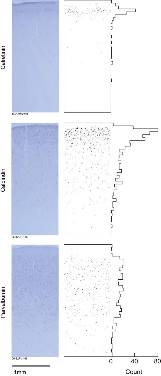
The distribution of GABAergic interneurons in SEF. Left, Shows coronal sections through SEF immunohistochemically reacted for the calcium binding proteins indicated. Right, Plots the location of positive neurons identified using a semi-automatic classification routine (see Materials and Methods) with associated histograms of cell counts as a function of depth. Calretinin and calbindin neurons are densest in layer II with diminishing deeper density, while parvalbumin neurons are more uniformly distributed across layers.

Results

Using linear microelectrode arrays (150 μm intercontact spacing), we recorded visually evoked and saccade-related LFPs and spikes from SEF of two macaque monkeys. We acquired 12,342 trials (6448 monkey E, 5894 monkey X) across 17 sessions (7 monkey E, 10 monkey X). The number of sessions is similar to that used in previous studies that recorded CSD from striate cortex (Maier et al., 2010; Maier et al., 2011; Spaak et al., 2012), although the number of trials per session is somewhat larger.

SEF was located through intracortical electrical microstimulation to elicit eye movements (Schlag and Schlag-Rey, 1987; Schall, 1991; Tehovnik et al., 1999; Martinez-Trujillo et al., 2004; Fig. 3a,b). To obtain CSD, we verified that electrode arrays entered the cortex perpendicular to the cortical surface through combined MR and CT imaging (Fig. 3c–j). After the electrode array had settled in the cortex (3–4 h), we presented wide-field (40 × 36° visual angle) light flashes (34.80 cd/m²) in blocks of 100–200 presentations, similar to stimuli used previously to characterize laminar microcircuitry in visual cortex (Schroeder et al., 1998; Maier et al., 2010). Interleaved with these blocks of visual stimulation, we recorded activity during spontaneous eye movements produced while the monkeys rested in darkness for periods of 5–10 min.

Single-session visually evoked CSD

Figure 4 shows data collected during a representative session. To interpret the CSD, it was necessary to estimate the depth of the electrode array relative to gray matter as described (see Materials and Methods). Several physiological measures provided information about electrode position. First, an artifact associated with the cardiac rhythm (hereafter referred to as the pulse artifact) was observed on a superficial channel. This signal indicated where the electrode was in contact with either the dura mater or the epidural saline in the recording chamber, which pulsated visibly with the monkeys' heartbeat. Second, across all sessions, we observed a marked increase of power in the γ frequency range (40–80 Hz) at several electrode contacts, which diminished gradually at deeper locations. Several recent studies have shown elevated γ power in superficial and middle layers relative to deep layers (Maier et al., 2010; Xing et al., 2012; Smith and Sommer, 2013), suggesting that this measure provides another useful marker for estimating depth. Finally, we recorded well isolated single units simultaneously with the LFPs, and colocalized their position with the markers described above. This set of diverse physiological signals provided converging evidence to evaluate the electrode position with regard to laminar depths that were assigned through the automated alignment procedure (described in Materials and Method and below).

Figure 4.

Raw and processed data from a representative session (1316 trials). a, Schematic diagram of electrode array drawn to scale and positioned on Nissl section from SEF (adapted from Matelli et al., 1991 with permission). b, Three seconds of raw LFP recorded from each of the contacts. The red trace (eighth from top) shows pulse artifact. c, LFP bandpass filtered from 40 to 80 Hz. Blue traces show γ activity elevated above the mean. d, Normalized mean γ power recorded at each electrode contact across session (blue) compared with average γ power recorded across all contacts (vertical black line). Note the pronounced increase in γ power at the contacts in the neuropil. e, Summary figure showing depth of pulse artifact (red line), elevated γ power (blue line), and the number of well isolated single units (black triangles) recorded simultaneously. During this session, we recorded 29 well isolated single units with 2 units on 5 channels and 3 units on another 5 channels. f, Three hundred milliseconds of event-related LFP aligned to the flash stimulus (vertical black line). Note the reversal in voltage polarity occurring on the channel with the pulse artifact. Above this channel the signal is volume-conducted EEG in the saline filling the recording chamber. Below this channel, the signals represent the electrocorticogram recorded from the pial surface and the LFPs recorded from the gray matter. g, Three hundred milliseconds of CSD derived from the LFPs, interpolating between contacts with 10 μm resolution. Vertical black line shows onset of flash stimulus.

Based on the known thickness of individual layers in SEF (Matelli et al., 1991), we estimated laminar boundaries and assigned visually evoked current sinks to specific layers (see Materials and Methods). In the representative recording session, the largest sink (minimum = −42 nA/mm³) occurred in layer III starting ∼50 ms after presentation of the stimulus. A second sink (minimum = −25 nA/mm³) began a few milliseconds later in layer V. A later sink (minimum = −23 nA/mm³) occurred more superficially in layers I/II, and additional weaker sinks (minimum = −20 nA/mm³) were evident in layer VI.

Several current sources are also apparent, including one at the level of the pulse artifact. Consistent with previous research, we interpret this source as passive current returning to the sinks below because it was recorded at the same level as the pulse artifact, and therefore, cannot have a cortical origin (Mitzdorf, 1985). In general, current sources can be caused either by passive return current or dendritic hyperpolarization making them harder to interpret than current sinks (Nicholson and Freeman, 1975; Mitzdorf, 1985). We therefore focus on current sinks for the remainder of this study.

To increase the SNR, we averaged the evoked CSD patterns across recording sessions, analogous to creating grand-average ERPs from EEG data, as done previously (Maier et al., 2010; Riera et al., 2012). To do this in an unbiased, data-driven manner, we developed an automated depth alignment procedure to maximize similarity between recording sessions using the entire source and sink laminar structure and timing. This mathematically optimized solution for depth alignment relies on the sole assumption that there are reliable similarities in CSD measured across recording sessions (see Materials and Methods). Figure 5 shows the results of this procedure with data from every recording session. The absolute magnitude of CSD varied from day to day and between monkeys, but in every session, we observed a clear sink in layer III ∼50 ms after the visual stimulus (Fig. 5b). In 15 of 17 sessions (88%) we also observed a second sink in layer V, and in 16 of 17 sessions (94%) we observed a third sink in layers I/II. On several recording sessions we placed the electrode array too superficially to sample from layer VI, but we observed a sink in this location in 11 of 13 sessions (85%). These consistencies validate the assumption that CSD is reliable across recording sessions and monkeys. Notably, the automated alignment technique was blind to the physiological signals detailed above (i.e., pulse artifact, LFP γ power, and single-unit locations), because it relied solely on the CSD data. Nevertheless, we observed a close correspondence between its estimates of cortical depth and the other physiological signals observed in the raw data, lending further support for the accuracy of this approach (Fig. 5c). Additional evidence for the accuracy of this automated alignment procedure comes from our findings of neural responses that differ by layer in SEF (see below).

Figure 5.

Results of the automated procedure for aligning U-probe recordings across sessions. A, Visually evoked CSD recorded individually for each session. The monkey and location of each penetration are indicated above. The recordings are aligned from left to right in chronological order within each monkey. Numbers near the top indicate the scales of the CSD maps (nA/mm³). Horizontal black bars indicate the estimated average location of gray matter based on the physiological signals. b, Visually evoked CSDs masked to show locations of the four grand-averaged, visually evoked sinks reported in Figure 6. Note the close correspondence in location of these sinks across recording sessions demonstrating the similarity in CSD recorded on subsequent days, and the success of our automated alignment procedure. c, Physiological signals apparent in the raw data on individual sessions. Pulse artifact (red lines), elevated γ activity (blue lines), and single units (black triangles) show good correspondence with our estimate of the location of gray matter (gray shading).

Grand-average visually evoked CSD

To ensure that data from both monkeys contributed equally to the grand-averaged CSD while preserving its absolute magnitude, we normalized the data so that the SD of each monkey's averaged CSD matched the SD of the grand-averaged CSD. We verified that the same qualitative pattern of results was observed when the data were not normalized, but report the results from this approach because it provides an average less prone to being driven by outliers. Visually evoked current sinks were observed across 2 mm of recording depth (Fig. 6a). Due to the placement of the electrode array, deeper channels were sampled less often than superficial channels (N = 17 channels 1–12, N = 15 channel 13, N = 13 channel 14–15, N = 11 channel 16). The peak magnitude of −25 nA/mm³ is only ∼15% of the magnitude of visually evoked current flow reported for primary visual cortex using similar stimulation parameters and recording and analysis techniques (Maier et al., 2010). Nevertheless, a clear laminar sequence of current sinks was apparent. Two initial sinks were observed in the grand average CSD, suggesting that visual afferents terminate in two distinct laminae. These findings agree with published anatomy (Matelli et al., 1991). Although it lacks a granular layer, SEF contains two layers of relatively dense pyramidal cells, one in deep layer III and a second forming layer V, which both receive visual afferents (Maioli et al., 1998; Shipp et al., 1998 see Discussion).

Figure 6.

Grand-average, visually evoked (left) and saccade-related (right) CSD from SEF. Nissl section from SEF in center indicates laminar architecture (adapted from Matelli et al., 1991 with permission). a, CSD recorded while monkeys passively viewed wide-field flashes of light. Four current sinks were observed and are numbered in order of appearance. b, CSD recorded while monkeys made spontaneous saccades in darkness. c, d, Data from a and b reproduced without interpolation highlighting time periods when channels deviate significantly from baseline (running Wilcoxon, p < 0.05 for > 5 consecutive 10 ms time bins). Sixteen channel depths are shown.

We used two methods to measure the onset latency of sinks in each layer (see Materials and Methods). First, we assessed differences from baseline using a running Wilcoxon approach. This method is quite sensitive, but only yields a single latency measure across sessions for each layer. The first sink (min −25 nA/mm³) appeared in layer III 51 ms after the stimulus, becoming maximal after 72 ms. The second sink (min −22 nA/mm³) developed in layer V at 55 ms, becoming maximal after 105 ms. Subsequent sinks occurred in layers I/II (min −14 nA/mm³) at 147 ms (peaking at 168 ms) and in layer VI (min −10 nA/mm³) at 172 ms (peaking at 173 ms). We also measured the onset latencies of laminar sinks in individual sessions by recording the time at which the sink reached 33% maximum. Although this method is somewhat less sensitive being unable to identify subtle onsets, it yields a useful estimate of variability across recording sessions. Using this approach, we recorded the following mean latencies ± SEM: layer III 50 ± 3 ms, layer V 73 ± 7 ms, layers I/II 100 ± 12 ms, layer VI 159 ± 25 ms.

To quantify these observations, we divided the time course following visual presentation into early (51–150 ms) and late (151–250 ms) epochs and conducted a hierarchical, repeated-measures ANOVA using layers, epochs, and monkeys as fixed factors and session number as a random factor nested within the fixed factor of monkey (Self et al., 2013). We observed significant differences in CSD by layer (F_(3,129) = 9.87, p = 4.73 × 10⁻⁵), and a decrease in CSD across layers during the late epoch (F_(1,129) = 166.28, p = 1.51 × 10⁻¹⁰). A significant main effect between monkeys was also observed showing that CSD tended to be larger in magnitude for monkey E (F_(1,129) = 21.91, p = 2.75 × 10⁻⁴). No significant effects were noted for the nested random factor of penetration number (F_(15,129) = 0.57, p = 0.86). Importantly, a significant interaction between layers and time periods was observed in the grand-average CSD (F_(3,129) = 21.96, p = 6.55 × 10⁻⁹). As an additional test, we conducted across-session running Wilcoxon tests on channels binned by the interelectrode spacing (150 μm). All four current sinks differed significantly from baseline (Fig. 6c). Thus, even though the current density was weaker than that observed in early sensory cortex, the pattern of synaptic current in the middle layers followed by current in superficial and deep layers was consistent across sessions and was similar though not identical to CSD obtained in early sensory cortex (Mitzdorf and Singer, 1978; Schroeder et al., 1998; Lakatos et al., 2007; Lipton et al., 2010; Riera et al., 2012).

Saccade-related CSD

To determine whether this pattern of current sinks is specific to visual input or occurs with other events during which SEF is modulated, we derived CSD associated with self-generated saccadic eye movements in darkness. The saccade-related CSD on individual sessions was very weak, but after alignment and averaging we observed distinct sinks (Fig. 6b,d). To ensure that presaccadic modulation could be detected if present, we also analyzed the 200 ms period immediately before saccade initiation. No significant current was detected during this time period. Although SEF neurons tend to have contralateral movement fields (Schall, 1991), no channels showed significant differences between ipsiversive and contraversive saccades [Wilcoxon rank sum, all ps > 0.05], so we describe the findings collapsed across saccade direction. Saccade-related CSD was weak, postsaccadic, and concentrated in the upper layers, peaking in layer III (min −9 nA/mm³) 32 ms after saccade initiation and more superficially (min −10 nA/mm³) after 162 ms. The absence of a strong presaccadic sink in layer V is consistent with other evidence that SEF does not contribute directly to saccade production (Stuphorn et al., 2010). Thus, the pattern of current sinks elicited by visual stimulation is specific to visual input.

Single units recorded using the linear microelectrode array

We recorded spiking activity from 295 single units simultaneously with the LFPs (115 monkey E, 180 monkey X). Few researchers have reported single-unit data recorded with the newly developed electrode array used in the current study (Hansen and Dragoi, 2011; Hansen et al., 2012). Therefore, we include a description of spike metrics, including the quality of isolation using a false-positive and false-negative estimate and a description of spike waveforms by depth, as well as measures of spike width and spiking variability as functions of recording depth.

Figure 7 shows principal component analysis (PCA) space and associated waveforms from example sessions taken from each monkey. These data show that the electrode array was capable of isolating single units effectively. We quantified isolation by estimating the number of false-positive and false-negative spiking events detected for each putative single unit (Hill et al., 2011a). In all, 88% of putative single units yielded false-positive rates below 10%, and 95% yielded false-positive rates below 20%. Also, 53% of putative single units yielded false-negative rates below 10%, and 81% yielded false-negative rates below 20%. These results are comparable to isolation metrics reported in other studies using the same methods (Hill et al., 2011b; Jacobs et al., 2013). However, the false-positive rate is somewhat lower showing that our single-unit data had very little false-positive contamination, and the false-negative rate is somewhat higher than those reported previously suggesting that we underestimated neural spiking with strict sorting criteria. Together, these measures suggest that we adopted a conservative approach in assigning spikes to single-unit clusters. The low false-positive rate supports our claim that single-unit recordings reflect the activity of individual neurons, but the relatively high false-negative rate suggests that we underestimated the firing rate of some of these neurons. In sum, these results show that the U-probe is capable of isolating activity of single neurons with performance comparable to that of traditional tungsten electrodes.

Figure 7.

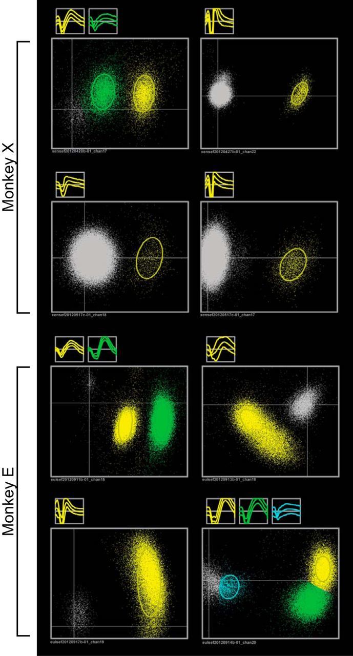
Sample waveforms and projected PCA space for eight sorted channels. Gray clouds represent multi-unit activity (unsorted threshold crossings). Channels 1–4 are from recordings with monkey X and channels 5–8 are from recordings with monkey E.

Spiking amplitude cannot be used as a reliable measure of neural morphology, because this metric is affected both by the size of a neuron and its proximity to the recording electrode, but other waveform metrics can provide insight. For instance, the number of peaks in a spike waveform can indicate which segment of the neuron contributed to the recording. Biphasic waveforms are common and tend to be recorded from cell bodies or the initial segment of the axon hillock, whereas triphasic waveforms are rare in neuropil because they are usually recorded from axons (for review, see Lemon, 1984). We noted a substantial proportion of triphasic waveforms while recording with the U-probe (39 of 295, 13%). These units were usually transient and were not isolated for long. This is a hallmark of axon recordings because the extracellular potentials of axons are many times smaller than those generated by cell somas, and an electrode must therefore lie very close to an axon to detect its activity (Lemon, 1984). We speculate that the U-probe must be suitable for recording the activity of axons because of the geometry of the electrode contacts. Unlike traditional tungsten microelectrodes in which the recording surface is sharp, the smooth electrode contacts on the U-probe shaft can be placed in close proximity to an axon without piercing or damaging it. We quantified the number of biphasic and triphasic single neurons recorded from each layer of cortex and from white matter (see Materials and Methods). Of the 36 single units recorded from layer II, none displayed triphasic waveforms. A very small proportion (5 of 116, 4%) of single units recorded in layer III displayed triphasic waveforms. Larger proportions of triphasic waveforms were detected in layers V (11 of 90, 12%) and VI (11 of 31, 35%). In white matter most waveforms were triphasic (12 of 22, 55%), suggesting that many of these responses were recorded from axons and fewer were recorded from interstitial neurons directly beneath layer VI (Suárez-Solá et al., 2009). Since it was impossible to determine the layer whence these putative axons originated, we excluded them from further analysis.

Spike width is another useful waveform metric that has been used to classify neurons as either putative pyramidal cells or putative interneurons (Constantinidis et al., 2002; Barthó et al., 2004; Mitchell et al., 2007; Cohen et al., 2009; but see Vigneswaran et al., 2011). We measured spike widths excluding units with triphasic waveforms (Mitchell et al., 2007). The overall distribution of spike widths was similar to that reported for V4 (Mitchell et al., 2007) and frontal eye field (FEF; Cohen et al., 2009) using similar criteria (Fig. 8). We assessed variability in firing rates by calculating coefficients of variation measured on interspike intervals (Cohen et al., 2009). Consistent with the hypothesized association between narrow spikes and interneurons, we found that narrow-spiking units displayed greater variability in spike timing than broad-spiking units [wide-spiking unit N = 203, narrow-spiking unit N = 53, Wilcoxon rank sum W = 23971, p = 1.06 × 10⁻⁵]. This result was identical when we restricted our analysis to single units with false-positive rates < 5% [wide-spiking unit N = 170, narrow-spiking unit N = 36, Wilcoxon rank sum W = 16214, p = 2.15 × 10⁻⁵]. These findings provide new evidence supporting the biophysical distinction between narrow- and broad-spiking units in agranular cortex. Across the pooled sample of single units, we found a small but significant correlation between spike width and recording depth (r₍₂₅₄₎ = 0.15 p = 0.01). Separate regression analyses on the narrow- and broad- spiking units revealed that broad-spiking units were the primary source of this effect. Broad-spiking units increased in width with recording depth (r₍₂₀₁₎ = 0.42 p = 6.47 × 10⁻¹⁰), while narrow-spiking units remained of the same width across depth (r₍₅₁₎ = 0.07 p = 0.60). These results were identical when we restricted our analysis to units with false-positive rates < 5% (wide-spiking unit r₍₁₆₈₎ = 0.44 p = 1.77 × 10⁻⁹; narrow-spiking unit r₍₃₄₎ = 0.13 p = 0.46). The finding of increased spike width for broad-spiking neurons as a function of depth is in agreement with anatomy; large pyramidal neurons are more prevalent in deeper layers. The incidence of narrow-spiking neurons corresponded to the density of parvalbumin but not of calretinin- or calbindin-expressing neurons in SEF (Fig. 9). This finding opens the interesting possibility that narrow-spiking units may primarily be parvalbumin-expressing interneurons since these are found throughout all layers in SEF and tend to have larger cell bodies.

Figure 8.

Biophysical characteristics of single units. a, All biphasic waveforms in population. Red and blue denote narrow and broad spikes, respectively (split at 250 μs). This color code is the same in the remaining parts. b, Cumulative probability distributions of CV of interspike intervals plotted separately for broad-spiking and narrow-spiking units. Narrow-spiking units showed more variability in spike timing. c, Spike width as a function of recording depth. Scatter plot shows regression of spike width by depth separated by broad- and narrow-spiking populations. Histograms show distributions of broad- and narrow-spiking units across each dimension. Broad-spiking units increased in width with depth. No such trend was observed for narrow-spiking units. d, Counts of broad-spiking and narrow-spiking units recorded in each layer.

Visually evoked spiking activity

The CCM hypothesis makes detailed predictions about spiking activity (Douglas and Martin, 1991; Douglas et al., 1995). First, excitation followed by suppression is proposed to be a common feature of the CCM. Second, excitatory and inhibitory neurons receive synchronized inputs; otherwise, recurrent excitatory connections would lead to unrestricted excitation. Third, in an effect mediated by relative differences in expression of GABA_A and GABA_B receptors, intracellular recordings in primary visual cortex show that pyramidal cells in superficial layers reach a maximum state of hyperpolarization later than those in deep layers. These predictions were tested in SEF by measuring visually evoked discharge rates of single- and multi-units recorded simultaneously with the LFPs. Of the single units recorded, 103 (35%) showed clear modulation following presentation of the flashed stimulus (63 monkey E, 40 monkey X). We also recorded thresholded multi-unit activity with clear visually evoked responses at 58 locations (42 monkey E, 16 monkey X). We included this multi-unit activity in our latency analyses but excluded it in analyses where spike width was used to classify neuron types.

Visually responsive units were recorded in all layers of SEF (Fig. 10, Table 1). As reported before (Schlag and Schlag-Rey, 1987; Schall, 1991; Chen and Wise, 1995), some units showed spiking enhancement (80, 50%) and others showed spiking suppression (81, 50%) following visual stimulus onset. We performed a 4 × 2 ANOVA to determine whether the latency of these responses differed between layers (four levels) and response types (two levels, i.e., enhancement vs suppression). Latencies were significantly shorter for units with enhanced responses than for units with suppressed responses (F_(1,149) = 16.62, p = 7.6 × 10⁻⁵). Thus, collectively, spiking activity in SEF exhibited a visually evoked wave of excitation followed by suppression. The latencies of visually evoked unit responses were not significantly different across layer (F_(3,149) = 1.18, p = 0.32), nor was an interaction between layer and response type evident (F_(3,149) = 0.53, p = 0.66). Thus, the temporal and spatial pattern of excitation and suppression in SEF is consistent with the first prediction of the CCM model.

Figure 10.

Single and multi-unit visually evoked response latencies to flashed stimuli. a, Representative units recorded from layer II (red), layer III (green), layer V (blue), and layer VI (black) demonstrating either enhanced (left) or suppressed discharge (right) rates following the stimulus. Shaded areas indicate the 95% confidence intervals measured across stimulus presentations. Vertical lines mark response latencies. b, Cumulative distributions of unit response latencies separated by layer and response type. Enhanced responses showed shorter latencies than suppressed responses. See also Table 1.

Table 1.

Summary statistics of units with visual responses recorded from each layer

Layer	# of SU	# of MU	Enhancement latencies	Suppression latencies
II	12	12	78 (53)	120 (45)
III	41	17	84 (41)	119 (41)
V	33	12	82 (37)	99 (38)
VI	17	17	89 (51)	120 (47)

SU, single units; MU, multi-units. Latencies are means (SD).

Seventy-seven broad-spiking units and 15 narrow-spiking units showed clearly detectable onset times (means ± SD, 107 ± 43 ms broad-spiking units, 97 ± 43 ms narrow-spiking units). To test whether excitatory and inhibitory neurons likely receive synchronized inputs, we determined whether putative pyramidal cells and interneurons in SEF show similar latencies. Consistent with the CCM model, onset times did not differ significantly between broad-spiking and narrow-spiking units [Wilcoxon rank sum W = 3664, p = 0.38]. To ensure that spike widths were appropriately estimated from well isolated single units, we repeated this analysis after discarding units with false-positive rates > 5%. This criterion excluded 14 putative pyramidal cells and 4 putative interneurons. Identical results were obtained with this subset [Wilcoxon rank sum W = 2410, p = 0.48].

To test whether superficial and deep layers can be distinguished based on the timing of hyperpolarization, we determined whether the maximum visually evoked spike suppression followed a longer time course in neurons recorded from upper versus lower layers in SEF. This is analogous to intracellular recordings showing that the time of maximum hyperpolarization is later in superficial layer neurons than in deep layer neurons of primary visual cortex (Douglas and Martin, 1991). Further, because this result is based on laminar differences in the relative pyramidal neuron expression of GABA_A and GABA_B receptors, we predicted that this effect would be restricted to broad-spiking units only. Extracellular recordings in SEF confirmed these predictions (Fig. 11). We limited this analysis to visually related units that showed decreased spiking after stimulus onset relative to baseline. The time of maximum spike suppression recorded from units in layers II and III (mean ± SD, 144 ± 61 ms), was significantly later than the time of maximum spike suppression from units recorded in layers V and VI (mean ± SD, 115 ± 62 ms) [Wilcoxon rank sum W = 2387, p = 4.30 × 10⁻³]. We further probed this effect by analyzing broad-spiking and narrow-spiking units separately. As predicted, broad-spiking neurons recorded in superficial layers showed significantly later maximum spike suppression than broad-spiking neurons recorded in deep layers [Wilcoxon rank sum W = 1719, p = 3.5 × 10⁻³], but this was not observed for narrow-spiking units [Wilcoxon rank sum W = 58, p = 0.80]. We repeated this analysis using only well isolated single units displaying false-positive rates < 5%. This criterion eliminated 11 and 2 broad-spiking units from superficial and deep layers, respectively, and 3 narrow-spiking units from superficial layers. Identical results were obtained with this subset. Broad-spiking units in superficial layers still showed later maximum spike suppression [Wilcoxon rank sum W = 1042, p = 0.01], and this result remained absent for narrow-spiking units [Wilcoxon rank sum W = 28, p = 0.95]. Adding evidence for differences in inhibition between layers, the overall probability of recording units with suppressed responses was also higher in superficial layers as reflected by a significant difference in depth by response type [Wilcoxon rank sum W = 6509, p = 5.28 × 10⁻⁴]. Thus, the time course and distribution of visually evoked spike suppression in SEF is consistent with the CCM model.

Figure 11.

Latency to maximum spike suppression differentiated by neuron depth and spike width. Superficial layers (II and III) versus deep layers (V and VI) and broad-spiking units (in blue) versus narrow-spiking units (in red). Error bars indicate SEM. Left, An example unit illustrating the measurement of latency to maximum spike suppression. Upper right inset shows the broad- and narrow-spiking units that make up the sample. A statistically significant difference was observed in the latency to maximum spike suppression between broad units recorded in superficial layers and broad units recorded in deep layers. No other comparisons differed significantly.

Saccade-related spiking activity

Units with saccade-related modulation were also recorded from all layers of SEF. We recorded 27 single units (9%) with activity related to spontaneous saccades made in darkness (14 monkey E, 13 monkey X). Ten of these neurons (37%) also displayed visually evoked activity. We additionally recorded saccade-related multi-unit activity from 24 locations (12 monkey E, 12 monkey X). Seventeen of these multi-unit recordings (71%) also displayed visually evoked activity. Of these 51 saccade-related units, 23 (45%) showed presaccadic modulation and 28 (55%) showed postsaccadic responses. In addition, 26 units (51%) showed increased firing rates before and during saccades while the remaining 25 (49%) showed suppression. Neither depth (mean = 0.38 mm relative to current sink 1, SD = 0.67 mm, Wilcoxon rank sum W = 17323, p = 0.64), nor spike widths (mean = 350 μs, SD = 99 μs, Wilcoxon rank sum W = 5224, p = 0.44), nor the coefficients of variation in interspike intervals (mean CV = 1.42, SD CV = 0.49, Wilcoxon rank sum W = 6597, p = 0.39), differed significantly between visually related and saccade-related units. A 4 × 2 ANOVA showed that latencies did not differ across layers (F_(3,43) = 1.12, p = 0.35), unlike visually responsive neurons, the latencies of enhanced and suppressed responses did not differ significantly (F_(1,43) = 1.09, p = 0.30) nor did the interaction between depth and response type (F_(3,43) = 2.04, p = 0.12). Table 2 presents summary statistics for this neural population separated by layer. Overall, these results demonstrate a relative lack of saccade-related activity in SEF when saccades are initiated without visible goals.

Table 2.

Summary statistics of units with saccade-related activity recorded from each layer

Layer	# of SU	# of MU	Enhancement latencies	Suppression latencies
II	4	5	−27 (46)	7 (43)
III	12	8	27 (52)	−6 (41)
V	7	5	22 (41)	29 (55)
VI	4	6	−3 (46)	48 (45)

SU, single units; MU, multi-units. Latencies are means (SD).

Discussion

We report CSD and laminar single- and multi-unit activity recorded from monkey SEF, an agranular area in the frontal lobe. Many results are consistent with the CCM formulated to explain granular sensory areas. However, some aspects of the data are inconsistent with the CCM. In particular, dual current sinks appeared nearly simultaneously in layers III and V and visual response latencies did not vary across layers.

CCM in SEF?

The laminar pattern of CSD in agranular SEF corresponds in many ways to the pattern predicted by the CCM model developed from data collected in granular primary visual cortex (Fig. 1a; Gilbert, 1983; Callaway, 1998; Douglas and Martin, 2004). After stimulus onset, current sinks in SEF began in middle layers and spread to superficial and deep layers. However, unlike in sensory cortical areas, two initial sinks were visible in SEF following visual stimulation corresponding to layers III and V. Although this result was anticipated based on anatomical tracer studies (reviewed below), it is unexpected based on the classic CCM model in which activity in a single input layer precedes activity in other layers.

In addition to feedforward activity, the CCM model also describes how local recurrent excitation amplifies ascending input while inhibition prevents uncontrolled excitation (Fig. 1b). Ascending input excites both pyramidal cells and interneurons leading to a characteristic pattern of excitation followed by suppression (Douglas and Martin, 1991; Douglas et al., 1995; see also Brunel and Wang, 2001; Chance et al., 2002; Haider et al., 2006). Consistent with this, we found enhanced discharge rates preceding suppression by ∼30 ms in all layers of SEF. We also found that putative pyramidal neurons (broad-spiking units) and putative interneurons (narrow-spiking units) were equally likely to display an initial enhancement in spiking following visual stimulation and that onset latencies did not differ between these populations.

Intracellular recordings highlight differences in the time course of maximum hyperpolarization between superficial and deep pyramidal cells mediated by GABA_A and GABA_B receptors (Douglas and Martin, 1991). Consistent with these results, we found that units recorded in superficial layers were more likely to respond to visual stimuli with suppression, and we noted a longer time course for maximum discharge rate suppression in superficial layers compared with that recorded in deep layers. This effect was restricted to putative pyramidal cells, suggesting laminar differences in GABA_A versus GABA_B expression in this cell type alone can account for the results. To avoid confusion, we note that our measures are analogous but not identical to those reported previously. Although Douglas and Martin (1991) measured the time of maximum hyperpolarization of intracellular potentials in primary visual cortex of anesthetized cats after electrical stimulation of thalamic afferents, we recorded discharge rate suppression from extracellular potentials in SEF of awake monkeys while presenting visual stimulation. Given these differences of technique, species, and area, the similarities in findings across studies suggest that this could be a general feature of mammalian neocortex.

Relation to previous anatomical studies

Fast visual input may be transmitted to SEF via the mediodorsal nucleus (MD) of the thalamus (Huerta and Kaas, 1990; Shook et al., 1990) that is innervated by the superior colliculus (Benevento and Fallon, 1975; Harting et al., 1980). But MD projections cannot explain the initial current sink we observed in layer V because afferents terminate in lower layer III of SEF (Giguere and Goldman-Rakic, 1988). Visual afferents to SEF are also supplied by cortical areas, including the lateral intraparietal area, area 7a, the FEF, the superior temporal polysensory area, visual area 6a (V6a), and the medial superior temporal area (MST; Barbas and Pandya, 1987; Huerta and Kaas, 1990; Shipp et al., 1998). Areas like MST and V6a likely provide fast visual input to SEF (Schmolesky et al., 1998). Consistent with our results, orthograde tracer injections in MST (Maioli et al., 1998) and in V6a (Shipp et al., 1998) reveal terminals in layers III and V in SEF. Also, consistent with our observation that layer VI is the last layer to show visually related CSD, projections from dorsal stream areas terminate only sparsely in layer VI of SEF (Maioli et al., 1998; Shipp et al., 1998). Thus, the laminar distribution of current sinks in response to visual stimulation is in good agreement with known anatomy.

Studying the CCM may reveal a cortical hierarchy in agranular cortex much as it has in granular cortex (Felleman and Van Essen, 1991). Shipp (2005) proposed that the ratio of layer III to layer V projections can be used to place agranular areas in an areal hierarchy. Our finding of relatively short latency, driving input to layers III and V of SEF is consistent with this hypothesis. These current sinks in SEF had similar latency and magnitude after visual stimulation suggesting both layers receive visual afferents of similar strength.

Relation to previous intracranial recording studies

Wide-field flashed stimuli such as those used here have been used to compare laminar activation profiles across successive stages of the visual hierarchy (Schroeder et al., 1989; Givre et al., 1994; Schroeder et al., 1998). The average latency of visually evoked CSD in SEF (51 ms) agrees with the work of Schroeder et al. (1998) who measured CSD throughout the visual pathway and reported the longest latencies in inferotemporal cortex (49 ms). Our CSD latency measure is also comparable to those of visually evoked LFPs in SEF during a visual search task (Purcell et al., 2012). Additionally, the latencies of single- and multi-unit responses observed here are consistent with several previous reports (Schall, 1991; Chen and Wise, 1995; Pouget et al., 2005; Purcell et al., 2012).

In early visual areas, response latencies are shortest in layer IV and longer in supragranular and infragranular layers (Bullier and Henry, 1980; Maunsell and Gibson, 1992; Raiguel et al., 1999). Recording in primary visual cortex, several groups have reported that latencies in supragranular layers are longer than those observed in deep layers (Maunsell and Gibson, 1992; Self et al., 2013). In SEF single- and multi-unit visual latencies did not differ across layers. This result is unanticipated based on the CCM model. The stimuli we used may have played a role in producing this puzzling result. While the wide-field flash paradigm we used is a necessary step for comparing CSD to published reports from early visual areas, it is somewhat less effective at driving action potentials in single- and multi-units in SEF (Fig. 10a). Because changes in firing rate were modest, our latency estimates may have had increased variability. However, the variability we observed was comparable to that reported in a study that used localized, behaviorally relevant visual stimuli (Pouget et al., 2005). The authors of that study detected latency differences of 37 ms in SEF. However, granular and supragranular layers in primary visual cortex exhibit latency differences of only ∼10–15 ms (Maunsell and Gibson, 1992), so latency differences between layers may be more difficult to detect in SEF. Thus, this null result should not be interpreted as definitive.

Response suppression was a common feature in our neural recordings. Several researchers have noted suppression of neural activity in SEF (Schlag and Schlag-Rey, 1987; Schall, 1991; Chen and Wise, 1995). The proportion of units displaying suppression varies across studies, but this may depend on stimulus parameters and task contingencies. The suppression we observed may also arise from receptive field surrounds. Center/surround receptive field architecture has not been characterized in SEF, but this has been reported in FEF (Schall et al., 2004; Cavanaugh et al., 2012).

Our measurements of spike width and variability in SEF are consistent with measures from other visual areas using similar metrics (Mitchell et al., 2007; Cohen et al., 2009). Our proportion of narrow-spiking to broad-spiking units (79%) is comparable to that reported in V4 (73%; Mitchell et al., 2007). Additionally, narrow-spiking units in SEF displayed increased spike-time variability providing new evidence that these cells represent interneurons.

Summary and conclusions

These data highlight the rich, multimodal information that can be obtained as advances in electrode array technology allow researchers to record well isolated single units with LFPs across cortical layers. We found that several features of visually evoked laminar responses in agranular SEF correspond to those observed in granular sensory areas. Crucially, pronounced current sinks were evident in the middle layers of SEF. The depth of these sinks provides a marker against which to measure the depth of each recorded neuron in vivo. This advance will undoubtedly prove crucial in describing neural interactions within intact, behaving monkeys.

References

- Barbas H, Pandya DN. Architecture and frontal cortical connections of the premotor cortex (area 6) in the rhesus monkey. J Comp Neurol. 1987;256:211–228. doi: 10.1002/cne.902560203. [DOI] [PubMed] [Google Scholar]
- Barthó P, Hirase H, Monconduit L, Zugaro M, Harris KD, Buzsáki G. Characterization of neocortical principal cells and interneurons by network interactions and extracellular features. J Neurophysiol. 2004;92:600–608. doi: 10.1152/jn.01170.2003. [DOI] [PubMed] [Google Scholar]
- Beckwith SVW, Stiavelli M, Koekemoer AM, Caldwell JAR, Ferguson HC, Hook R, Lucas RA, Bergeron LE, Corbin M, Jogee S. The Hubble ultra deep field. Astron J. 2006;132:1729–1755. doi: 10.1086/507302. [DOI] [Google Scholar]
- Benevento LA, Fallon JH. The ascending projections of the superior colliculus in the rhesus monkey (Macaca mulatta) J Comp Neurol. 1975;160:339–361. doi: 10.1002/cne.901600306. [DOI] [PubMed] [Google Scholar]
- Boynton GM. Spikes, BOLD, attention, and awareness: a comparison of electrophysiological and fMRI signals in V1. J Vis. 2011;11(5):1–16. doi: 10.1167/11.5.12. [DOI] [PMC free article] [PubMed] [Google Scholar]
- Brunel N, Wang XJ. Effects of neuromodulation in a cortical network model of object working memory dominated by recurrent inhibition. J Comput Neurosci. 2001;11:63–85. doi: 10.1023/A:1011204814320. [DOI] [PubMed] [Google Scholar]
- Bullier J, Henry GH. Ordinal position and afferent input of neurons in monkey striate cortex. J Comp Neurol. 1980;193:913–935. doi: 10.1002/cne.901930407. [DOI] [PubMed] [Google Scholar]
- Buzsáki G, Czopf J, Kondákor I, Kellényi L. Laminar distribution of hippocampal rhythmic slow activity (RSA) in the behaving rat - Current source density analysis, effects of urethane and atropine. Brain Res. 1986;365:125–137. doi: 10.1016/0006-8993(86)90729-8. [DOI] [PubMed] [Google Scholar]
- Callaway EM. Local circuits in primary visual cortex of the macaque monkey. Annu Rev Neurosci. 1998;21:47–74. doi: 10.1146/annurev.neuro.21.1.47. [DOI] [PubMed] [Google Scholar]
- Cavanaugh J, Joiner WM, Wurtz RH. Suppressive surrounds of receptive fields in monkey frontal eye field. J Neurosci. 2012;32:12284–12293. doi: 10.1523/JNEUROSCI.0864-12.2012. [DOI] [PMC free article] [PubMed] [Google Scholar]
- Chance FS, Abbott LF, Reyes AD. Gain modulation from background synaptic input. Neuron. 2002;35:773–782. doi: 10.1016/S0896-6273(02)00820-6. [DOI] [PubMed] [Google Scholar]
- Chen LL, Wise SP. Supplementary eye field contrasted with the frontal eye field during acquisition of conditional oculomotor associations. J Neurophysiol. 1995;73:1122–1134. doi: 10.1152/jn.1995.73.3.1122. [DOI] [PubMed] [Google Scholar]
- Cohen JY, Pouget P, Heitz RP, Woodman GF, Schall JD. Biophysical support for functionally distinct cell types in the frontal eye field. J Neurophysiol. 2009;101:912–916. doi: 10.1152/jn.90272.2008. [DOI] [PMC free article] [PubMed] [Google Scholar]
- Constantinidis C, Williams GV, Goldman-Rakic PS. A role for inhibition in shaping the temporal flow of information in prefrontal cortex. Nat Neurosci. 2002;5:175–180. doi: 10.1038/nn799. [DOI] [PubMed] [Google Scholar]
- Di S, Baumgartner C, Barth DS. Laminar analysis of extracellular field potentials in rat vibrissa barrel cortex. J Neurophysiol. 1990;63:832–840. doi: 10.1152/jn.1990.63.4.832. [DOI] [PubMed] [Google Scholar]
- Douglas RJ, Martin KA. A functional microcircuit for cat visual cortex. J Physiol. 1991;440:735–769. doi: 10.1113/jphysiol.1991.sp018733. [DOI] [PMC free article] [PubMed] [Google Scholar]
- Douglas RJ, Martin KA. Neuronal circuits of the neocortex. Annu Rev Neurosci. 2004;27:419–451. doi: 10.1146/annurev.neuro.27.070203.144152. [DOI] [PubMed] [Google Scholar]
- Douglas RJ, Koch C, Mahowald M, Martin KA, Suarez HH. Recurrent excitation in neocortical circuits. Science. 1995;269:981–985. doi: 10.1126/science.7638624. [DOI] [PubMed] [Google Scholar]
- Felleman DJ, Van Essen DC. Distributed hierarchical processing in the primate cerebral cortex. Cereb Cortex. 1991;1:1–47. doi: 10.1093/cercor/1.1.1. [DOI] [PubMed] [Google Scholar]
- Freeman JA, Nicholson C. Experimental optimization of current source-density technique for anuran cerebellum. J Neurophysiol. 1975;38:369–382. doi: 10.1152/jn.1975.38.2.369. [DOI] [PubMed] [Google Scholar]
- Geyer S, Zilles K, Luppino G, Matelli M. Neurofilament protein distribution in the macaque monkey dorsolateral premotor cortex. Eur J Neurosci. 2000;12:1554–1566. doi: 10.1046/j.1460-9568.2000.00042.x. [DOI] [PubMed] [Google Scholar]
- Giguere M, Goldman-Rakic PS. Mediodorsal nucleus: areal, laminar, and tangential distribution of afferents and efferents in the frontal lobe of rhesus monkeys. J Comp Neurol. 1988;277:195–213. doi: 10.1002/cne.902770204. [DOI] [PubMed] [Google Scholar]
- Gilbert CD. Microcircuitry of the visual cortex. Annu Rev Neurosci. 1983;6:217–247. doi: 10.1146/annurev.ne.06.030183.001245. [DOI] [PubMed] [Google Scholar]
- Givre SJ, Schroeder CE, Arezzo JC. Contribution of extrastriate area V4 to the surface-recorded flash VEP in the awake macaque. Vision Res. 1994;34:415–428. doi: 10.1016/0042-6989(94)90156-2. [DOI] [PubMed] [Google Scholar]
- Godlove DC, Garr AK, Woodman GF, Schall JD. Measurement of the extraocular spike potential during saccade countermanding. J Neurophysiol. 2011a;106:104–114. doi: 10.1152/jn.00896.2010. [DOI] [PMC free article] [PubMed] [Google Scholar]
- Godlove DC, Emeric EE, Segovis CM, Young MS, Schall JD, Woodman GF. Event-related potentials elicited by errors during the stop-signal task. I. macaque monkeys. J Neurosci. 2011b;31:15640–15649. doi: 10.1523/JNEUROSCI.3349-11.2011. [DOI] [PMC free article] [PubMed] [Google Scholar]
- Haider B, Duque A, Hasenstaub AR, McCormick DA. Neocortical network activity in vivo is generated through a dynamic balance of excitation and inhibition. J Neurosci. 2006;26:4535–4545. doi: 10.1523/JNEUROSCI.5297-05.2006. [DOI] [PMC free article] [PubMed] [Google Scholar]
- Hansen BJ, Dragoi V. Adaptation-induced synchronization in laminar cortical circuits. Proc Natl Acad Sci U S A. 2011;108:10720–10725. doi: 10.1073/pnas.1102017108. [DOI] [PMC free article] [PubMed] [Google Scholar]
- Hansen BJ, Chelaru MI, Dragoi V. Correlated variability in laminar cortical circuits. Neuron. 2012;76:590–602. doi: 10.1016/j.neuron.2012.08.029. [DOI] [PMC free article] [PubMed] [Google Scholar]
- Harting JK, Huerta MF, Frankfurter AJ, Strominger NL, Royce GJ. Ascending pathways from the monkey superior colliculus: an autoradiographic analysis. J Comp Neurol. 1980;192:853–882. doi: 10.1002/cne.901920414. [DOI] [PubMed] [Google Scholar]
- Heinen SJ, Liu M. Single-neuron activity in the dorsomedial frontal cortex during smooth-pursuit eye movements to predictable target motion. Vis Neurosci. 1997;14:853–865. doi: 10.1017/S0952523800011597. [DOI] [PubMed] [Google Scholar]
- Heinzle J, Hepp K, Martin KA. A microcircuit model of the frontal eye fields. J Neurosci. 2007;27:9341–9353. doi: 10.1523/JNEUROSCI.0974-07.2007. [DOI] [PMC free article] [PubMed] [Google Scholar]
- Helmstaedter M, de Kock CP, Feldmeyer D, Bruno RM, Sakmann B. Reconstruction of an average cortical column in silico. Brain Res Rev. 2007;55:193–203. doi: 10.1016/j.brainresrev.2007.07.011. [DOI] [PubMed] [Google Scholar]
- Hill DN, Mehta SB, Kleinfeld D. Quality metrics to accompany spike sorting of extracellular signals. J Neurosci. 2011a;31:8699–8705. doi: 10.1523/JNEUROSCI.0971-11.2011. [DOI] [PMC free article] [PubMed] [Google Scholar]
- Hill DN, Curtis JC, Moore JD, Kleinfeld D. Primary motor cortex reports efferent control of vibrissa motion on multiple timescales. Neuron. 2011b;72:344–356. doi: 10.1016/j.neuron.2011.09.020. [DOI] [PMC free article] [PubMed] [Google Scholar]
- Huerta MF, Kaas JH. Supplementary eye field as defined by intracortical microstimulation - connections in macaques. J Comp Neurol. 1990;293:299–330. doi: 10.1002/cne.902930211. [DOI] [PubMed] [Google Scholar]
- Jacobs J, Weidemann CT, Miller JF, Solway A, Burke JF, Wei XX, Suthana N, Sperling MR, Sharan AD, Fried I, Kahana MJ. Direct recordings of grid-like neuronal activity in human spatial navigation. Nat Neurosci. 2013;16:1188–1190. doi: 10.1038/nn.3466. [DOI] [PMC free article] [PubMed] [Google Scholar]
- Kajikawa Y, Schroeder CE. How local is the local field potential? Neuron. 2011;72:847–858. doi: 10.1016/j.neuron.2011.09.029. [DOI] [PMC free article] [PubMed] [Google Scholar]
- Lakatos P, Chen CM, O'Connell MN, Mills A, Schroeder CE. Neuronal oscillations and multisensory interaction in primary auditory cortex. Neuron. 2007;53:279–292. doi: 10.1016/j.neuron.2006.12.011. [DOI] [PMC free article] [PubMed] [Google Scholar]
- Lemon R. Methods for neuronal recording in conscious animals. New York: Wiley; 1984. [Google Scholar]
- Lipton ML, Liszewski MC, O'Connell MN, Mills A, Smiley JF, Branch CA, Isler JR, Schroeder CE. Interactions within the hand representation in primary somatosensory cortex of primates. J Neurosci. 2010;30:15895–15903. doi: 10.1523/JNEUROSCI.4765-09.2010. [DOI] [PMC free article] [PubMed] [Google Scholar]
- Logothetis NK. What we can do and what we cannot do with fMRI. Nature. 2008;453:869–878. doi: 10.1038/nature06976. [DOI] [PubMed] [Google Scholar]
- Logothetis NK, Kayser C, Oeltermann A. In vivo measurement of cortical impedance spectrum in monkeys: implications for signal propagation. Neuron. 2007;55:809–823. doi: 10.1016/j.neuron.2007.07.027. [DOI] [PubMed] [Google Scholar]
- Maier AV, Adams GK, Aura C, Leopold DA. Distinct superficial and deep laminar domains of activity in the visual cortex during rest and stimulation. Front Syst Neurosci. 2010;4:31. doi: 10.3389/fnsys.2010.00031. pii. [DOI] [PMC free article] [PubMed] [Google Scholar]
- Maier A, Aura CJ, Leopold DA. Infragranular sources of sustained local field potential responses in macaque primary visual cortex. J Neurosci. 2011;31:1971–1980. doi: 10.1523/JNEUROSCI.5300-09.2011. [DOI] [PMC free article] [PubMed] [Google Scholar]
- Maioli MG, Squatrito S, Samolsky-Dekel BG, Riva Sanseverino ER. Corticocortical connections between frontal periarcuate regions and visual areas of the superior temporal sulcus and the adjoining inferior parietal lobule in the macaque monkey. Brain Res. 1998;789:118–125. doi: 10.1016/S0006-8993(98)00025-0. [DOI] [PubMed] [Google Scholar]
- Markov NT, Misery P, Falchier A, Lamy C, Vezoli J, Quilodran R, Gariel MA, Giroud P, Ercsey-Ravasz M, Pilaz LJ, Huissoud C, Barone P, Dehay C, Toroczkai Z, Van Essen DC, Kennedy H, Knoblauch K. Weight consistency specifies regularities of macaque cortical networks. Cereb Cortex. 2011;21:1254–1272. doi: 10.1093/cercor/bhq201. [DOI] [PMC free article] [PubMed] [Google Scholar]
- Markram H. The blue brain project. Nat Rev Neurosci. 2006;7:153–160. doi: 10.1038/nrn1848. [DOI] [PubMed] [Google Scholar]
- Martinez-Trujillo JC, Medendorp WP, Wang H, Crawford JD. Frames of reference for eye-head gaze commands in primate supplementary eye fields. Neuron. 2004;44:1057–1066. doi: 10.1016/j.neuron.2004.12.004. [DOI] [PubMed] [Google Scholar]
- Matelli M, Luppino G, Rizzolatti G. Architecture of superior and mesial area-6 and the adjacent cingulate cortex in the macaque monkey. J Comp Neurol. 1991;311:445–462. doi: 10.1002/cne.903110402. [DOI] [PubMed] [Google Scholar]
- Maunsell JH, Gibson JR. Visual response latencies in striate cortex of the macaque monkey. J Neurophysiol. 1992;68:1332–1344. doi: 10.1152/jn.1992.68.4.1332. [DOI] [PubMed] [Google Scholar]
- Mitchell JF, Sundberg KA, Reynolds JH. Differential attention-dependent response modulation across cell classes in macaque visual area V4. Neuron. 2007;55:131–141. doi: 10.1016/j.neuron.2007.06.018. [DOI] [PubMed] [Google Scholar]
- Mitzdorf U. Current source-density method and application in cat cerebral-cortex - Investigation of evoked-potentials and EEG phenomena. Physiol Rev. 1985;65:37–100. doi: 10.1152/physrev.1985.65.1.37. [DOI] [PubMed] [Google Scholar]
- Mitzdorf U, Singer W. Prominent excitatory pathways in cat visual-cortex (A17 and A18) - Current source density analysis of electrically evoked-potentials. Exp Brain Res. 1978;33:371–394. doi: 10.1007/BF00235560. [DOI] [PubMed] [Google Scholar]
- Mitzdorf U, Singer W. Excitatory synaptic ensemble properties in the visual-cortex of the macaque monkey–current source density analysis of electrically evoked-potentials. J Comp Neurol. 1979;187:71–83. doi: 10.1002/cne.901870105. [DOI] [PubMed] [Google Scholar]
- Nicholson C, Freeman JA. Theory of current source-density analysis and determination of conductivity tensor for anuran cerebellum. J Neurophysiol. 1975;38:356–368. doi: 10.1152/jn.1975.38.2.356. [DOI] [PubMed] [Google Scholar]
- Olson CR, Gettner SN. Object-centered direction selectivity in the macaque supplementary eye field. Science. 1995;269:985–988. doi: 10.1126/science.7638625. [DOI] [PubMed] [Google Scholar]
- Paxinos G, Huang X-F, Toga AW. The rhesus monkey brain in stereotaxic coordinates. San Diego: Academic; 2000. [Google Scholar]
- Pettersen KH, Devor A, Ulbert I, Dale AM, Einevoll GT. Current-source density estimation based on inversion of electrostatic forward solution: effects of finite extent of neuronal activity and conductivity discontinuities. J Neurosci Methods. 2006;154:116–133. doi: 10.1016/j.jneumeth.2005.12.005. [DOI] [PubMed] [Google Scholar]
- Pouget P, Emeric EE, Stuphorn V, Reis K, Schall JD. Chronometry of visual responses in frontal eye field, supplementary eye field, and anterior cingulate cortex. J Neurophysiol. 2005;94:2086–2092. doi: 10.1152/jn.01097.2004. [DOI] [PubMed] [Google Scholar]
- Pouget P, Stepniewska I, Crowder EA, Leslie MW, Emeric EE, Nelson MJ, Schall JD. Visual and motor connectivity and the distribution of calcium-binding proteins in macaque frontal eye field: implications for saccade target selection. Front Neuroanat. 2009;3:2. doi: 10.3389/neuro.05.002.2009. [DOI] [PMC free article] [PubMed] [Google Scholar]
- Purcell BA, Weigand PK, Schall JD. Supplementary eye field during visual search: salience, cognitive control, and performance monitoring. J Neurosci. 2012;32:10273–10285. doi: 10.1523/JNEUROSCI.6386-11.2012. [DOI] [PMC free article] [PubMed] [Google Scholar]
- Raiguel SE, Xiao DK, Marcar VL, Orban GA. Response latency of macaque area MT/V5 neurons and its relationship to stimulus parameters. J Neurophysiol. 1999;82:1944–1956. doi: 10.1152/jn.1999.82.4.1944. [DOI] [PubMed] [Google Scholar]
- Riera JJ, Ogawa T, Goto T, Sumiyoshi A, Nonaka H, Evans A, Miyakawa H, Kawashima R. Pitfalls in the dipolar model for the neocortical EEG sources. J Neurophysiol. 2012;108:956–975. doi: 10.1152/jn.00098.2011. [DOI] [PubMed] [Google Scholar]
- Schall JD. Neuronal activity related to visually guided saccadic eye movements in the supplementary motor area of rhesus monkeys. J Neurophysiol. 1991;66:530–558. doi: 10.1152/jn.1991.66.2.530. [DOI] [PubMed] [Google Scholar]
- Schall JD, Godlove DC. Current advances and pressing problems in studies of stopping. Curr Opin Neurobiol. 2012;22:1012–1021. doi: 10.1016/j.conb.2012.06.002. [DOI] [PMC free article] [PubMed] [Google Scholar]
- Schall JD, Morel A, King DJ, Bullier J. Topography of visual cortex connections with frontal eye field in macaque: convergence and segregation of processing streams. J Neurosci. 1995;15:4464–4487. doi: 10.1523/JNEUROSCI.15-06-04464.1995. [DOI] [PMC free article] [PubMed] [Google Scholar]
- Schall JD, Sato TR, Thompson KG, Vaughn AA, Juan Ch. Effects of search efficiency on surround suppression during visual selection in frontal eye field. J Neurophysiol. 2004;91:2765–2769. doi: 10.1152/jn.00780.2003. [DOI] [PubMed] [Google Scholar]
- Schlag J, Schlag-Rey M. Evidence for a supplementary eye field. J Neurophysiol. 1987;57:179–200. doi: 10.1152/jn.1987.57.1.179. [DOI] [PubMed] [Google Scholar]
- Schmolesky MT, Wang Y, Hanes DP, Thompson KG, Leutgeb S, Schall JD, Leventhal AG. Signal timing across the macaque visual system. J Neurophysiol. 1998;79:3272–3278. doi: 10.1152/jn.1998.79.6.3272. [DOI] [PubMed] [Google Scholar]
- Schroeder CE, Tenke CE, Arezzo JC, Vaughan HG., Jr Timing and distribution of flash-evoked activity in the lateral geniculate nucleus of the alert monkey. Brain Res. 1989;477:183–195. doi: 10.1016/0006-8993(89)91406-6. [DOI] [PubMed] [Google Scholar]
- Schroeder CE, Mehta AD, Givre SJ. A spatiotemporal profile of visual system activation revealed by current source density analysis in the awake macaque. Cereb Cortex. 1998;8:575–592. doi: 10.1093/cercor/8.7.575. [DOI] [PubMed] [Google Scholar]
- Self MW, van Kerkoerle T, Supèr H, Roelfsema PR. Distinct roles of the cortical layers of area V1 in figure-ground segregation. Curr Biol. 2013;23:2121–2129. doi: 10.1016/j.cub.2013.09.013. [DOI] [PubMed] [Google Scholar]
- Shipp S. The importance of being agranular: a comparative account of visual and motor cortex. Philos Trans R Soc Lond B Biol Sci. 2005;360:797–814. doi: 10.1098/rstb.2005.1630. [DOI] [PMC free article] [PubMed] [Google Scholar]
- Shipp S, Blanton M, Zeki S. A visuo-somatomotor pathway through superior parietal cortex in the macaque monkey: cortical connections of areas V6 and V6A. Eur J Neurosci. 1998;10:3171–3193. doi: 10.1046/j.1460-9568.1998.00327.x. [DOI] [PubMed] [Google Scholar]
- Shook BL, Schlag-Rey M, Schlag J. Primate supplementary eye field. 1. Comparative aspects of mesencephalic and pontine connections. J Comp Neurol. 1990;301:618–642. doi: 10.1002/cne.903010410. [DOI] [PubMed] [Google Scholar]
- Smith MA, Sommer MA. Spatial and temporal scales of neuronal correlation in visual area V4. J Neurosci. 2013;33:5422–5432. doi: 10.1523/JNEUROSCI.4782-12.2013. [DOI] [PMC free article] [PubMed] [Google Scholar]
- Spaak E, Bonnefond M, Maier A, Leopold DA, Jensen O. Layer-specific entrainment of gamma-band neural activity by the alpha rhythm in monkey visual cortex. Curr Biol. 2012;22:2313–2318. doi: 10.1016/j.cub.2012.10.020. [DOI] [PMC free article] [PubMed] [Google Scholar]
- Stuphorn V, Taylor TL, Schall JD. Performance monitoring by the supplementary eye field. Nature. 2000;408:857–860. doi: 10.1038/35048576. [DOI] [PubMed] [Google Scholar]
- Stuphorn V, Brown JW, Schall JD. Role of supplementary eye field in saccade initiation: executive, not direct, control. J Neurophysiol. 2010;103:801–816. doi: 10.1152/jn.00221.2009. [DOI] [PMC free article] [PubMed] [Google Scholar]
- Suárez-Solá ML, González-Delgado FJ, Pueyo-Morlans M, Medina-Bolívar OC, Hernández-Acosta NC, González-Gómez M, Meyer G. Neurons in the white matter of the adult human neocortex. Front Neuroanat. 2009;3:7. doi: 10.3389/neuro.05.007.2009. [DOI] [PMC free article] [PubMed] [Google Scholar]
- Tehovnik EJ, Slocum WM, Schiller PH. Behavioural conditions affecting saccadic eye movements elicited electrically from the frontal lobes of primates. Eur J Neurosci. 1999;11:2431–2443. doi: 10.1046/j.1460-9568.1999.00665.x. [DOI] [PubMed] [Google Scholar]
- Thompson KG, Hanes DP, Bichot NP, Schall JD. Perceptual and motor processing stages identified in the activity of macaque frontal eye field neurons during visual search. J Neurophysiol. 1996;76:4040–4055. doi: 10.1152/jn.1996.76.6.4040. [DOI] [PubMed] [Google Scholar]
- Vigneswaran G, Kraskov A, Lemon RN. Large identified pyramidal cells in macaque motor and premotor cortex exhibit “thin spikes”: implications for cell type classification. J Neurosci. 2011;31:14235–14242. doi: 10.1523/JNEUROSCI.3142-11.2011. [DOI] [PMC free article] [PubMed] [Google Scholar]
- Xing D, Yeh CI, Burns S, Shapley RM. Laminar analysis of visually evoked activity in the primary visual cortex. Proc Natl Acad Sci U S A. 2012;109:13871–13876. doi: 10.1073/pnas.1201478109. [DOI] [PMC free article] [PubMed] [Google Scholar]