

Abstract
Diffusion tensor imaging (DTI) is unable to represent the diffusion signal arising from multiple crossing fascicles and freely diffusing water molecules. Generative models of the diffusion signal, such as multi-fascicle models, overcome this limitation by providing a parametric representation for the signal contribution of each population of water molecules. These models are of great interest in population studies to characterize and compare the brain microstructural properties. Central to population studies is the construction of an atlas and the registration of all subjects to it. However, the appropriate definition of registration and atlasing methods for multi-fascicle models have proven challenging. This paper proposes a mathematical framework to register and analyze multi-fascicle models. Specifically, we define novel operators to achieve interpolation, smoothing and averaging of multi-fascicle models. We also define a novel similarity metric to spatially align multi-fascicle models. Our framework enables simultaneous comparisons of different microstructural properties that are confounded in conventional DTI. The framework is validated on multi-fascicle models from 24 healthy subjects and 38 patients with tuberous sclerosis complex, 10 of whom have autism. We demonstrate the use of the multi-fascicle models registration and analysis framework in a population study of autism spectrum disorder.
Index Terms: Diffusion magnetic resonance imaging (MRI), interpolation, microstructure, multi-fascicle, multi-tensor, population studies, registration
I. Introduction
Diffusion magnetic resonance imaging enables in vivo investigation of the brain microstructure. Diffusion tensor imaging (DTI) has long been used in this context. However, DTI confounds the signal arising from different fascicles and from diffusion of free water, challenging the interpretation of scalar measures such as the fractional anisotropy (FA) and mean diffusivity (MD) [1]. This limitation makes DTI inadequate in the vast majority of the white matter since 60–90% of voxels contain more than one fascicle, according to recent estimates [2].
Various models have been proposed to overcome the limitations of DTI. Among them, generative models such as multi-tensor models [3], [4], CHARMED [5], NODDI [6] and DIAMOND [7] seek to represent the signal contribution from different populations of water molecules. These models are based on underlying biological assumptions and are of great interest to characterize and compare white-matter properties. For example, assessment of the free water diffusion arising from the extracellular space may be useful for the characterization of edema or inflammation [8]. A neuroinflammatory response may indeed lead to an increase in the amount of free diffusion [9]. Modeling of each individual fascicle may be useful to characterize properties such as the fascicle density, the axonal diameter distribution or the myelin integrity [10].
In this context, multi-tensor models are particularly interesting for three reasons. First, they enable the direct generalization of conventional measures computed from DTI (FA, MD, etc.) by enabling their computation for each fascicle independently. Second, they provide a model for the unrestricted water diffusion. Third, they can be estimated from short acquisition sequences that are clinically available [3], [11]. At each voxel, multi-tensor models represent the diffusion signal
 for a gradient direction g and a b-value b by:
| (1) |
where N is the maximum number of fascicles crossing in one voxel and fi is the volumetric fraction of fascicle i (with Σi fi = 1). Unrestricted water diffusion is represented as one of the compartments with an isotropic tensor (D = DisoI3).
Conducting population studies based on multi-fascicle models (MFM) requires the alignment of all models to a common coordinate system (the atlas). Registering and atlasing multi-tensor images are known to be challenging and many studies attempt to perform population analyses without resorting to them [12], [13], [14], [15]. In [12], a T2-weighted image of the subject is registered to a DWI at b = 0 and correspondence between subjects is achieved by segmenting the anatomy based on a T1-weighted atlas. In tract-based spatial statistics (TBSS) [13], single-tensor images are estimated and FA images are used to spatially align subjects. To interpret anisotropies in crossing fiber areas, heuristics based on the mode and FA of the tensor are used. In crossing-fiber TBSS [15], a ball-and-sticks model is estimated but spatial alignment is still based on single-tensor FA images. None of these approaches attempt to register multi-tensor models directly.
Direct registration of multi-fascicle models is important since the latter provide increased contrast in areas where T2-weighted images and FA images are almost constant (as will be shown in Section IV-C). Furthermore, multi-tensor image registration can be made invariant with respect to differences in FA and MD, which is important when those properties need to be compared after alignment. The challenges of registering and analyzing multi-fascicle models stems from difficulties in processing multi-tensors. In particular, interpolating, averaging, smoothing and defining robust similarity metrics for multi-fascicle models cannot be directly extended from the single-tensor case. This is because the j-th tensor in one voxel does not necessarily correspond to the same fascicle as the j-th tensor in another voxel. Furthermore neighboring voxels may contain different number of fascicles.
Interpolation and smoothing are required in registration to apply transforms and to prevent aliasing in multi-scale approaches. Building an atlas further requires averaging MFM. From a mathematical perspective, interpolating, smoothing and averaging all amount to computing weighted combinations of MFM. In this paper, we propose a mathematical framework to compute weighted combinations of MFM and a similarity metric to register them. These developments enable registration and analysis of multi-fascicle models which open new opportunities for population studies of microstructural properties. These contributions extend our previous work [16] by providing detailed derivations, experiments and discussions.
Section II introduces the mathematical framework to process multi-fascicle models. Section III details how the mathematical framework is applied to statistically analyze properties of the brain microstructure across populations. Section IV presents results on in vivo data. Finally, Section V concludes.
II. Material
This section introduces the components of the proposed mathematical framework for multi-fascicle models.
A. Weighted combinations of multi-fascicle models for interpolation, averaging and smoothing
Computing weighted combinations of multi-fascicle models is at the basis of interpolation, smoothing and averaging. The linear combination of K mixture models each with N components results in a mixture with KN components that we call the complete model:
| (2) |
| (3) |
In most practical applications, increasing from N to KN the number of components is not desirable. We therefore estimate a simplified model,
 , with N components which best approximates the complete model:
| (4) |
| (5) |
where D(·, ·) is some discrepancy measure between the complete and simplified models. This problem is known as mixture model simplification for which efficient approaches have recently been proposed [17], [18], [19]. In [17], the simplified mixture model is defined as that which minimizes the cumulative differential relative entropy between the complete and simplified models:
| (6) |
The variables πi cluster the components of the complete mixture into N clusters each represented by a single component of the simplified mixture, ; πi = j means that is best represented by . Banerjee et al. [17] showed that, as long as and belong to the exponential family, Equation (6) can be optimized in an expectation-maximization scheme for which both the E-step and the M-step can be solved in closed form (Fig. 1). This makes the computation of weighted combinations of multi-fascicle models tractable. Mixtures of distributions from the exponential family is a wide class of mixtures which includes Gaussian mixtures [4], ball-and-sticks models [20], composite hindered and restricted models [21], diffusion directions models [22], Watson and Bingham distributions [6].
Fig. 1.
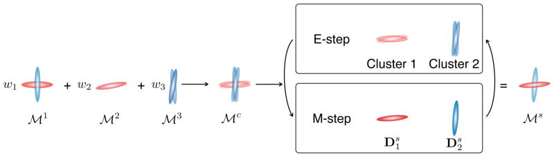
Computing weighted combinations of multi-fascicle models amounts to computing the complete mixture
 and simplifying it in an EM scheme to obtain
. The E-step is a clustering problem and the M-step consists in averaging log-tensors in each cluster.
and simplifying it in an EM scheme to obtain
. The E-step is a clustering problem and the M-step consists in averaging log-tensors in each cluster.
In the case of multi-tensor models, the E-step consists in optimizing for the clustering variables πi assuming are known, based on the Burg divergence B(·, ·) between covariances Σ = D−1:
| (7) |
The M-step then consists in optimizing the parameters of the simplified mixture (that is and ) to minimize (6) providing that we know πi. Davis and Dhillon [18] proved that this step amounts to computing the weighted average of covariance matrices and fractions in each cluster:
| (8) |
Alternating the E-step (7) and M-step (8) until convergence provides the parameters ( and ) of the weighted combination of mixtures. Initialization is required to control the local minimum to which EM will converge. We initialize the clustering variables πi by spectral clustering using the cosine similarity matrix between the primary eigenvector ei of each tensor [23]. We found this initialization to be efficient in our experiments. However, since the algorithm typically converges in a few steps, one may consider running it multiple times with various initializations and selecting the result that yields the lowest cumulative differential relative entropy.
One may be concerned about the swelling effect due to averaging covariance matrices in (8). This motivates the definition of a log-Euclidean version of the mixture model simplification described above, as it has been defined for single-tensor interpolation [24]. This is achieved by replacing the covariance matrices by their matrix logarithm before performing the EM. The update of the covariance matrices now reads:
Since log Σ = log D−1 = − log D, the logarithmic version of the weighted combination of multi-fascicle models is equivalent to its single-tensor counterpart in voxels with only one tensor. This is not the case in the Euclidean version since covariance matrices, rather than tensors, are averaged. A pseudocode of the method is presented in Algorithm 1.
Algorithm 1.
Weighted Combinations in one voxel
| 1: |
Input:
K multi-fascicle models
 with weights wk and the number N of fascicles in the output. with weights wk and the number N of fascicles in the output. |
| 2: | Output: A multi-fascicle model: |
| 3: |
for
k in 1 to K
do ▷ Construct the complete model
|
| 4: | for j in 1 to N do |
| 5: | i ← (k − 1)N + j |
| 6: | |
| 7: | |
| 8: | end for |
| 9: | end for |
| 10: | π ← Initialization ( ) ▷ Initialize clustering |
| 11: | while π has not converged do |
| 12: | for j in 1 to N do ▷ M-Step |
| 13: | |
| 14: | |
| 15: | end for |
| 16: | for i in 1 to KN do ▷ E-Step |
| 17: | for j in 1 to N do |
| 18: | |
| 19: | end for |
| 20: | πi ← arg minl Bi(l) |
| 21: | end for |
| 22: | end while |
Importantly, due to the construction of a complete model, the framework described above does not depend on the label i assigned to tensors in the multi-tensor model and accounts for cases where the number of tensors differs between voxels.
B. A generalized correlation coefficient as a similarity metric for multi-fascicle models
To register multi-fascicle models, a similarity metric between multi-tensor images needs to be defined. Since registration is used for population studies, the similarity metric must be invariant to inter-subject variability. In particular, since mean diffusivity and fractional anisotropy are typically used as potential biomarkers for diseases, the similarity metric must be invariant to changes in FA and MD. This observation has lead Zhang et al. to define a single-tensor similarity metric based on deviatoric tensors, making it invariant to changes in MD [25], though not robust to other differences in diffusivity profiles. In this section, we generalize the correlation coefficient widely used in scalar images when intensities differ between subjects and we show that this similarity metric is invariant under changes in FA and MD.
The correlation coefficient as a similarity metric for block matching is defined as the scalar product between the normalized blocks. For voxels with values in ℝ, the blocks R and S defined over a domain Ω with |Ω| voxels are elements of ℝ × … × ℝ = ℝ|Ω| and the correlation coefficient reads:
| (9) |
where μ is the mean of the image values in the block and 〈·, ·〉 is the canonical scalar product in ℝ|Ω|. It is invariant if R is replaced by aR + b.
For vector images with values in ℝn, blocks are elements of ℝn ×… ×ℝn = (ℝn)|Ω|. The correlation coefficient can be generalized to vector images by redefining the means μR and μS as the projection of the block onto a block T ∈ (ℝn)|Ω| that has a constant value at each voxel, i.e. T(x) = t0 ∀x [26]:
| (10) |
The factor 〈R, T〉/||T||2 is a scalar that we call the scalar mean and is equal to μR for scalar images. Equation (9) is therefore a particular case of (10) for n = 1 and t0 = 1. This generalized correlation coefficient can be used in any vector space endowed with an inner product. It is invariant if R is replaced by aR + bT where a and b are scalars and T is the chosen constant block.
Let us first generalize the correlation coefficient to single-tensor diffusion images which will prove useful for the generalization to multi-tensor images. Single-tensor blocks are elements of
, where
is the space of 3×3 symmetric positive definite matrices. It is typically more convenient to work in the log-tensor space in which blocks are elements of (
 )|Ω|. This space is endowed with the Frobenius inner product and the correlation coefficient of (10) can be readily applied. Choosing t0 = I3, the correlation coefficient is invariant under linear transformation of the log-tensor eigenvalues:
due to the invariance log D → log D′ = a log D + log bI3. It is instructive to observe what the definition of the scalar mean becomes in this space with the Frobenius inner product. We have:
)|Ω|. This space is endowed with the Frobenius inner product and the correlation coefficient of (10) can be readily applied. Choosing t0 = I3, the correlation coefficient is invariant under linear transformation of the log-tensor eigenvalues:
due to the invariance log D → log D′ = a log D + log bI3. It is instructive to observe what the definition of the scalar mean becomes in this space with the Frobenius inner product. We have:
| (11) |
| (12) |
| (13) |
| (14) |
The generalized scalar mean for blocks of single-tensors is therefore the logarithm of the geometric mean of diffusivities over the domain Ω.
Defining a scalar product in the space (
 )|Ω| of blocks of multi-tensors seems impractical if not impossible. We further generalize the correlation coefficient (10) by substituting the inner product 〈·, ·〉, by a more general scalar mapping: m(·, ·) :
 ×
→ ℝ for any space
. The generalized correlation coefficient becomes:
×
→ ℝ for any space
. The generalized correlation coefficient becomes:
where nm(X)2 = m(X, X) is a generalization of the norm, and T is assumed normalized (nm(T) = 1).
This expression does not guarantee the invariance of the generalized correlation coefficient (GCC) with respect to linear changes of the blocks: R → R′ = aR + bT. Furthermore, in order to remain interpretable, the GCC must be symmetric, equal to one in case of perfect match and lower than one in any other case:
| (15) |
| (16) |
| (17) |
| (18) |
These constraints on ρ impose constraints on the scalar mapping m. One can show that constraints (15–18) are satisfied if the following constraints are respected by m:
| (19) |
| (20) |
| (21) |
| (22) |
The latter generalizes the Cauchy-Schwartz inequality. Being a scalar product is a sufficient but unnecessary condition to respect these constraints. Therefore, constraints (19–22) as well as the choice of a constant block T and suitable basic operations (to define the multiplication by a scalar and the addition of the constant block T), stand together as a model to generate correlation coefficients in potentially any space, even when an inner product cannot be defined.
In the case of multi-fascicle models, we further want the similarity metric between two multi-tensor blocks and to be equal to the single-tensor similarity metric if the blocks contain only one tensor in each voxel. This can be achieved if the scalar mapping is equal to the Frobenius inner product when all but one fractions are equal to zero. We therefore add a fifth constraint on the scalar mapping:
| (23) |
We define the multiplication of multi-tensors by a scalar a as the multiplication of all log-tensors by a and the addition of the constant block T as the addition of t0 to all log-tensors. These definitions naturally generalize the single-tensor case. A generalized scalar mapping m comes by computing pairwise scalar products between corresponding tensors. This requires to pair tensors between the two blocks at each voxel. We introduce the following notation:
where p is the pairing function which associates one and only one tensor of
 to one and only one tensor of
 . For N–fascicle models, there are N! such pairings. We define the scalar mapping for multi-tensor images as:
| (24) |
In practice, the values of d(p, x) for all N! pairings p are computed and we select the one with the highest absolute value. This scalar mapping satisfies (19–23). The absolute value is required by Condition (23) for cases where the Frobenius inner product between the tensors is negative. To better interpret this generalized scalar mapping, it is instructive to assess how it generalizes the concept of scalar means and norm to multi-fascicle models. The generalized scalar mean is given by:
| (25) |
Remarkably, the generalized scalar mean for multi-fascicle model is the geometric mean of the diffusivities within the block for which all fascicles contribute in a ratio that is equal to their volumetric fraction fi in their voxel. As for the generalized norm of multi-fascicle models, it is given by:
| (26) |
that is the sum of the Frobenius norms of each log-tensor, weighted by the squared fractions. To demonstrate the latter expression, we need to show that the absolute value of d in (24) is maximized if the pairing p pairs a fascicle (in
 =
) with itself (in
=
) with itself (in
 =
). The proof is straightforward using the Cauchy-Schwartz inequality on elements X = (f1 log D1, …, fN log DN) and Yp = (fp(1) log Dp(1), …, fp(N) log Dp(N)). Both the generalized scalar mean and the generalized norm therefore have direct interpretations in terms of multi-fascicle models.
=
). The proof is straightforward using the Cauchy-Schwartz inequality on elements X = (f1 log D1, …, fN log DN) and Yp = (fp(1) log Dp(1), …, fp(N) log Dp(N)). Both the generalized scalar mean and the generalized norm therefore have direct interpretations in terms of multi-fascicle models.
More importantly, the proposed generalized scalar mapping leads to a GCC that is invariant under linear transformations of the eigenvalues of each log-tensor. In other words, ρ for multi-fascicle models is invariant under the following transformations (i = 1, 2, 3):
or, equivalently
| (27) |
for all fascicles. In particular, this invariance property encompasses differences in mean diffusivity (MD) for unchanged FA if a ≠ 1 and b = 1. Similarly, changes in FA with unchanged MD can be obtained by varying a and b in a specific manner. Indeed, MD is preserved under changes of the eigenvalues following Equation (27), if . For any given set of eigenvalues and any given a, there exists a b that satisfies this relation. One can therefore fix a to match the desired FA and subsequently fix b to respect this MD-preserving relation (since b does not affect the FA). Finally, by varying both a and b in an unconstrained manner, various changes in MD and FA can be accounted for by the invariance property of the GCC.
This similarity metric therefore allows registration of subjects with locally different diffusivity profiles. Importantly, because of the presence of the fractions f1 and f2 in the scalar mapping, the GCC accounts for cases where the number of tensors is different in different voxels (the corresponding fraction will simply be set to zero).
III. Methods
With the framework developed in the previous section, we can now perform population studies by constructing a multi-fascicle atlas and registering all subjects to it. From there, we can employ our novel operators including interpolation and averaging of multi-fascicle models to perform different statistical analyses of brain microstructural properties.
A. Registration and Atlasing
Multi-fascicle models are estimated in the coordinate system of a T1-weighted MRI of the same subject (see Section III-D). The registration between multi-fascicle models is initialized by affine registration of the T1-weighted MRI using the Baladin method [27], yielding a transformation T0.
The weighted combinations of multi-fascicle models and the GCC are introduced in a robust multi-scale block matching registration algorithm developed in [28]. A dense deformation field is estimated through the following steps:
-
For each pyramid level p = 1, …, P
-
For each iteration i = 1, …, N
Estimate sparse pairings C between R and F ∘ Ti−1 by block-matching
Interpolate a dense correction field δTi from C using a Gaussian kernel and weighted by the confidence in the matches as in [29].
Reject a fixed amount of outliers from C based on their dissimilarity with the estimated δTi
Estimate an outlier-free correction δT˜i
Compose the correction δT˜i with the current estimate of the transform Ti = Ti−1 ∘ δT˜i
Apply elastic regularization to the field Ti
-
In our implementation, P = 4, N = 10, block sizes are 5 × 5 × 5, and the outlier removal rate is 20%. The weighted combinations of multi-fascicle models are used to interpolate multi-tensor images when applying the deformation or constructing the multi-scale representation of the image. When warping tensor images (and hence multi-tensor images), tensors need to be reoriented. This reorientation is performed using the finite-strain rationale [30].
Registration is then used iteratively to build an atlas based on the method developed in [31]. This method essentially alternates between aligning and averaging images. To average multi-tensor images, we use the weighted combination of multi-fascicle models described above. Ten iterations are used to build the final atlas. The resulting atlas for single-tensor and multi-tensor images are depicted in Fig. 2.
Fig. 2.

Single-tensor and multi-fascicle atlases overlaid on the T1-weighted MRI atlas. The multi-fascicle atlas presents tensors with higher fractional anisotropies than the single-tensor atlas. This is due to the account of both the free water diffusion in the isotropic compartment and the multiple fascicle present in the voxel. The highlighted regions represent the corona radiata where projections of the corpus callosum cross cortico-spinal tracts, and a region where the pyramidal tracts (vertical lines) and the medial cerebellar peduncle (horizontal lines) cross.
B. Statistical Analysis: Fascicle-Based Spatial Statistics
With all subjects aligned to the multi-fascicle atlas, we can compare properties of the aligned tracts through fascicle-based spatial statistics (FBSS) (Fig. 3). Tractography is performed once on the atlas using the multi-fascicle tractography method described in [32], [33], [34] and adapted to include the multi-fascicle interpolation. For each registered subject, the tensor most aligned with the tract is selected and its property of interest (FA, MD, etc.) is computed. This provides, for each subject, a vector of length n (the number of points on the tract), representing the microstructural property along the fascicle.
Fig. 3.

Fascicle-based spatial statistics (FBSS) proceeds in three steps. (a) Fascicles (grey line) are drawn on the atlas with a sub-voxel resolution. The point in the middle is at a non-grid location. (b) Multi-fascicle models are interpolated at non-grid locations. (c) At each location along the fascicle, the tensor most aligned to the fascicle is selected to compute the property of interest (FA, MD, etc.).
Point-by-point t-tests are carried out along the tract to compare its properties between the two groups. This yields a vector t of n t-scores. Since the smoothness of the tract property depends on the individual, the tract and the resolution of the tractography, we use a non-parametric correction for multiple comparisons based on cluster-based statistics [35]. This method assumes that differences along the tract occur in clusters of adjacent points and proceeds as follows:
Define a threshold t0 on the t-statistics.
- Define a binary vector b of supra-threshold t-statistics:
Detect the connected components C = {ci} in b.
For each connected component ci, compute its size si (number of points) and its mass mi (sum of t-scores).
Randomly permute Np times the subjects in the groups (i.e. randomly reassign subjects to either groups) and perform Steps 1–4 for each permutation. For each permutation k, record the maximum size and the maximum mass among the detected clusters.
-
The recorded and describe the null distributions of the size and mass of the clusters. Corrected for multiple comparisons, the p-values of each connected component ci testing for its likelihood to be due to chance alone are:
for the size statistics and the mass statistics, respectively.
With FBSS, local fascicle segments where the two groups significantly differ can be discovered. Several t-thresholds t0 are typically used to assess the robustness of the findings. Higher t0 yield smaller clusters of stronger differences.
C. Statistical Analysis: Isotropic Diffusion Analysis
Large isotropic fraction fiso indicates an excessive extracellular volume [36] which is in turn a surrogate for the presence of edema or neuroinflammation [8]. Isotropic diffusion analysis (IDA), i.e. the statistical analysis of the isotropic fraction, is thus of strong interest for population studies of disease involving these pathologies. The isotropic fraction is non-Gaussian since it ranges between 0 and 1. We apply the logit transform to fiso prior to computing t-tests. This transform brings the distribution of fiso closer to normality. Specifically, we transform fiso-maps into liso-maps where:
To prevent liso to take on infinite values when fiso = 0 or 1, we bound the latter within [10−6, 1–10−6]. We then carry cluster-based statistics on the liso-maps with the cluster size and cluster masses as quantities of interest, as described in [35].
D. In vivo data
In vivo DWI were acquired on a Siemens 3T Trio scanner with a 32 channel head coil using the CUSP-45 gradient sequence [3]. This sequence includes 30 diffusion-encoding gradients on a shell at b = 1000s/mm2 and 15 extra gradients in the enclosing cube of constant TE with b-values up to 3000s/mm2. Eddy current distortion was minimized using a twice-refocused spin echo sequence [37]. Other acquisition parameters were set to FOV= 220mm, matrix= 128 × 128, number of slices=68, resolution = 1.7 × 1.7 × 2mm3. Data acquisition was conducted using a protocol approved by the Institutional Review Board (IRB). The DW images were aligned to the 1×1×1mm3 T1-weighted MRI with rigid registration (using the mean b = 0 image as a moving image) and the gradients were reoriented appropriately. This compensates for patient head motion and for residual geometric distortions due to magnetic field inhomogeneity and eddy current.
A multi-fascicle model with three tensors including an isotropic compartment were estimated as in [3]. Images were acquired for 24 healthy controls and 38 patients with tuberous sclerosis complex (TSC): 10 diagnosed with autism (TSC+ASD), 17 diagnosed without (TSC-ASD) and 11 too young for diagnosis.
IV. Results
In this section, we validate the presented framework for multi-fascicle models. We systematically compare our results with those obtained when multi-tensor images are seen as a stack of single-tensor images on which multi-channel approaches to registration and averaging can be applied.
A. Relabeling Invariance Study
Multi-fascicle models assign arbitrary labels i to tensors in Equation (1). The framework must therefore be invariant under relabeling of tensors. In this experiment, we randomly relabeled tensors 10 times for each of the 24 healthy controls and performed registration between the result and the original image. Using the proposed framework, the deformation fields obtained were exactly the identity. By contrast, using the multi-channel registration, a significantly non-zero deformation field resulted from the registration of relabeled multi-fascicle models (Fig. 4). This result demonstrates the failure of multi-channel registration for multi-fascicle models. In what follows, tensors are labeled based on their FA (D1 has the highest FA and DN the lowest) to allow a fair comparison between the two approaches.
Fig. 4.
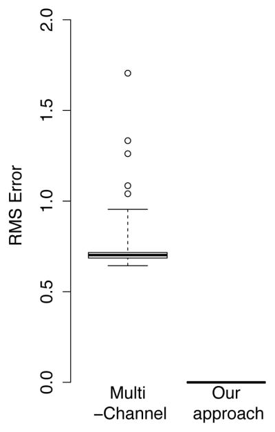
Average RMS error of the deformation fields obtained by registering a multi-fascicle model with itself after randomly relabeling tensors. Our framework is invariant under relabeling leading to an error that is exactly zero. By contrast, multi-channel registration yields non-zero deformation fields.
B. T−1 ∘ T Study: Assessment of the Interpolation Error
For any transformation T, the composition T−1 ∘ T is equal to the identity. Therefore, for any image A, T−1 ∘ T ∘ A = A. However, if we first compute (T ∘ A) and then apply T−1 to the result, we do not obtain exactly the original image A due to interpolation error. Comparing the result A˜ = T−1 ∘ (T ∘ A) to the original A thus provides estimates of the interpolation error, independently from the similarity metric.
We investigated the residual error of T−1∘T∘A to compare the interpolation error of the proposed approach for linear combinations and the multi-channel alternative. The experiment was conducted with three different affine transformations T that were applied to the multi-fascicle models of the 24 healthy controls: (1) a transformation that maps the DWI to the T1-weighted image, (2) a translation by half a voxel in all directions, (3) a rotation of 45 degrees around the vertical axis.
The result A ˜ is compared to the original multi-fascicle model A in terms of the following four similarity metric computed at each voxel:
| (28) |
| (29) |
| (30) |
| (31) |
where e1,i is the principal eigenvector of tensor Di with unit norm. The last equation assesses how aligned the resulting tensors are to the original tensors.
The results, summarized in Fig. 5, demonstrate that the use of the proposed method decreases the interpolation error as compared to the multi-channel alternative, for all similarity metrics and for all three transformations. On average, this decrease varies in magnitude from 38% for ΔMD to 73% for ΔDir. One-tailed paired t-tests indicate that the decreases are significant in all cases (p < 10−12). An example of interpolation obtained with both methods is depicted in Fig. 6 and presents a portion of the corona radiata where fascicles cross. In this region, the multi-channel approach confounds the fascicles and fails to interpolate the multi-fascicle model.
Fig. 5.

Estimation of the interpolation errors demonstrates the superiority of the proposed approach compared to the multi-channel alternative to compute linear combinations of multi-fascicle models. The bar plots show the interpolation error for four metrics (ΔFA, ΔMD, Fro and ΔDir) under three different transformations.
Fig. 6.

(Left) Performing interpolation for each tensor independently (considered as channels of a multi-channel image) confounds fascicles resulting in an inflated result. (Right) Weighted combination of multi-fascicle models introduced in our mathematical framework clusters similar fascicles to avoid the inflation effect. (a–b) Results obtained on synthetic data by interpolating the multi-fascicle models at the extremities. (c–d) Results obtained on in vivo data by applying a linear transform to a multi-fascicle model.
C. Scan-Rescan Study: Evaluation of the Similarity Metric
In this section, we independently assess the accuracy of the similarity metric. We exploited two sets of 45 DWI acquired on the same subject during the same scanning session. The subject was required not to move and remained still throughout the acquisition. The two sets of DWI are thus intrinsically aligned. A multi-fascicle model as well as a single-tensor DTI were estimated from each set. The two multi-fascicle models differ due to acquisition noise, artifacts, and estimation errors. This scan-rescan experiment therefore provides a unique opportunity to estimate the accuracy of the proposed similarity metric in a realistic scenario.
A total of 495 landmarks were defined on a regular grid within the first image (Fig. 7(a)). Landmarks were spaced 7 voxels apart in all directions. Blocks of size 5 × 5 × 5 were defined around each landmark and correspondence were sought in a neighborhood of size 21 × 21 × 21 in the second image. Since there is no transformation between the two images, the true correspondence xtrue is located at the center of the neighborhood. The accuracy of the best match xmax (that maximizes the similarity C(x)) and the saliency of the true match are:
| (32) |
where C̄ and σc are the mean and standard deviation of the similarity metric within the neighborhood.
Fig. 7.

The GCC for multi-fascicle models outperforms other metrics in terms of registration accuracy, as assessed by a scan-rescan experiment. (a) 495 regularly spaced landmarks are used for the experiment. (b) Similarity maps in four neighborhoods (circles indicate true matches) showing that GCC is the most specific metric. (c) In regions with no contrast in FA, the GCC is able to find correct matches due to robust patterns observed in multi-fascicle models. (d) The accuracy of the GCC is significantly better than all other metrics as seen by the cumulative distribution function (CDF). (e) No significant difference in saliency between the metrics are observed, except for a significantly higher saliency with CDTI.
Results for these two indices were compared amongst four different metric (1) the correlation coefficient applied to FA images (CFA), (2) the correlation coefficient generalized to single-tensor DTI (CDTI), (3) the multi-channel correlation coefficient applied to multi-tensors (CMC) and the GCC for multi-fascicle models (GCC). Fig. 7(b) depicts the similarity maps for four different neighborhoods with each metric.
Neighborhood 1 in Fig. 7(b) illustrates the case of a specific white matter landmark, for which all four metrics perform equally well. Neighborhood 2 illustrates a case of a specific white matter landmark located at the intersection of crossing fascicles. In this case, both metrics based on multi-fascicle models find the correct match. Matching based on FA has more spurious maxima and matching based on DTI is offset because the single-tensor is a poor model of the diffusion signal in this region. Finally, Neighborhoods 3 and 4 show landmarks located at the boundary between the white and grey matter. In this area the microstructure is more complex. Multi-fascicle models are required in these regions to find a correct match. The multi-channel metric fails to detect the correct correspondence if tensors are not properly paired (see Neighborhood 4).
Fig. 7(c) depicts the volumetric fraction (shown as a color image) in areas where the FA displays no contrast. The fractions show a clear pattern of alternation between isotropic diffusion (blue) and single (green) or multi-fascicle (brown) orientation. These patterns are repeated in both the scan and the rescan and therefore enable accurate matching.
Quantitatively, the GCC for multi-fascicle models significantly outperforms all other metrics in terms of accuracy (one-tailed paired t-test: p < 10−8), as depicted in Fig. 7(d) and summarized in Table I. The average gain in accuracy CFA is 45%. Importantly, the probability for the accuracy to be lower or equal to 1, that is the fraction of landmarks for which the best match was found in the direct neighborhood of the true match, is P (Accuracy ≤ 1) > 80% for the GCC while it is lower than 70% for all other metrics. These results suggest that the remaining registration error would likely be eliminated by regularization and outlier removal in the registration algorithm. No significant difference was observed in terms of saliency except for a significantly larger saliency for CDTI which may partially counterbalance its poorer accuracy in registration.
TABLE I.
Summary statistics of the target registration error in the scan-rescan study
| Metric | Mean | St. dev. | P(Accuracy ≤1) |
|---|---|---|---|
|
| |||
| CFA | 1.79 | 2.79 | 67.3% |
| CDTI | 2.18 | 3.05 | 59.4% |
| CMC | 3.34 | 4.18 | 47.5% |
| GCC | 0.98 | 1.66 | 83.4% |
D. Comparison with Single-Tensor DTI Registration
As an alternative to the proposed approach for registration, one may suggest to register single-tensor DTI and use the resulting deformation fields to deform the multi-fascicle models. Such a method would not require any similarity metric between multi-tensors but would still require our framework to apply the deformation field to the multi-fascicle models. In this experiment, however, we illustrate that directly registering multi-fascicle models is more accurate than registering DTI.
We compared DTI registration and multi-fascicle registration under the application of a synthetic deformation field. Using a full dataset of 45 DWI form one subject, resampled to the T1-weighted space at a resolution of 1 mm×0.86 mm×0.86 mm, we estimated both a DTI and a multi-fascicle model. Both models were deformed by the same random synthetic log-Euclidean polyaffine transform (the true field) obtained by drawing parameters from a Gaussian with zero mean and 0.05 standard deviation for 27 regularly spaced affine components (this results in a field with a mean magnitude of 6.9 voxels and a maximum magnitude of 42 voxels) [38]. The single-tensor registration was performed using DTI-TK (version 2.3.1) [25] with the default parameters and after properly rescaling tensors. The multi-fascicle registration was performed using our framework. The resulting fields were applied to the original multi-fascicle model and the results were compared, in terms of metrics (28)–(31), to the multi-fascicle model deformed by the true field. We also computed the norm (Δfield) of the difference between the deformation field obtained by registration and the true field. All comparisons were conducted within a mask that excludes the background.
In terms of all five metrics, registering the multi-fascicle models with our framework significantly improves the alignment accuracy compared to single-tensor registration with DTI-TK (one-sided paired t-test: p < 10−6 for all six metrics) as depicted on Fig. 8(a). The differences in accuracy between the two approaches are mostly visible in areas with crossing fascicles, such as the corona radiate as shown in the zoomed-in areas of Fig. 8(b). In these regions, single-tensor DTI have low contrast and DTI-TK is therefore less reliable than our approach which takes advantage of the full multi-fascicle model in the registration.
Fig. 8.

Registering multi-fascicle models with our framework leads to higher alignment accuracies than registering single-tensor DTI with DTI-TK. (a) Quantitative assessment shows that registration errors using our framework are significantly lower than those obtained with DTI-TK [25]. (b) The difference in registration error is mostly visible in areas with crossing fascicles, where single-tensor DTI models have low contrast compared to multi-fascicle models. The zoomed-in areas are located in the corona radiata.
E. Synthetic Fields Study
In this experiment, we compare the registration accuracies when synthetic deformation fields are applied to multi-fascicle models. Ten random log-Euclidean polyaffine deformation fields are generated by drawing parameters from a Gaussian with zero mean and 0.05 standard deviation for 27 regularly spaced affine components [38]. Each of the ten deformations are applied to the 24 multi-fascicle models of the control subjects. Symmetric matrices of Gaussian noise with zero mean and standard deviation at six different levels (0.1, 0.2, 0.3; and 0.5, 1.0, 1.5) were then added to the log of all tensors in both the original and the transformed image, corresponding to SNR of (30dB, 24dB, 21dB, 17dB, 11dB, 7dB). The original and the transformed images were then registered and the resulting deformation field was compared to the initial synthetic field in term of its root mean squared (RMS) error. All 1,440 registrations (24 subjects × 10 deformation fields × 6 noise levels) were performed with both the proposed framework and the multi-channel alternative.
On average, the root mean squared (RMS) error of the deformation field is 17% higher when the multi-channel registration is used instead of the proposed framework. A one-tailed paired t-test on the RMS for the transformation at each SNR shows that the difference in RMS between the approaches is significant: p < 10−5 for all SNR between 11dB and 30dB and p = 0.02 for SNR=7dB (Fig. 9-Top). The variance of the RMS is also decreased by 45% on average. A one-tailed F-test reveals that this decrease is significant for all SNR (p < 0.001) except for SNR=24dB and 7dB (Fig. 9-Bottom). This experiment indicates that even when tensors are labeled based of their FA, the proposed framework outperforms the multi-channel alternative.
Fig. 9.

Our mathematical framework leads to higher registration accuracies than the multi-channel alternative: the RMS errors (top) and its variance (bottom) are significantly lower. Results are shown for 1,440 registrations performed at various SNR for synthetic deformation fields (* p < 0.05, ** p < 0.005, *** p < 0.001).
F. Morphometric Contrast Study
The deformation field obtained by registering a subject to an atlas provides a measurement of the local morphometric difference between the subject and a standard anatomy. The determinant of the Jacobian |J| of the deformation fields at every voxel provides information about the amount of local volume differences (|J| < 1 indicates a decreased volume and |J| > 1 indicates an increased volume).
Widespread volume deficits in the white and grey matter of patients with TSC have been previously reported [39]. However, the amount of differences detected depends on the accuracy of the registration because the statistical power of the test depends on the registration accuracy [40]. Because of the increased level of microstructure they represent, we expect multi-fascicle models to reveal more morphometric differences than single-tensor models and scalar T1-weighted MRI. To assess the statistical power of all modalities (T1, single-tensor DTI and multi-fascicle models), we used the common voxel-based morphometry method [41]: register all subjects to the atlas, compute the log-jacobian, smooth it by a kernel of 8mm FWHM and correct for family-wise error rate at p = 0.05.
Results in Fig. 10(a) show that multi-fascicle models reveal more differences than single-tensors and T1-weighted MRI, as expected. This is likely due to an increased statistical power resulting from a higher registration accuracy when the structure of the white matter is better represented. The number of significant voxels does not differ between the proposed approach and the multi-channel alternative. However, the spatial distribution of the volume deficit findings (Fig. 10(b)) better follows the anatomy than the multi-channel alternative as seen, for example, in the left and right internal capsules.
Fig. 10.

Morphometry results show areas with a significant volume deficit within the grey and white matter of TSC patients. (a) Multi-fascicle registration and multi-channel registration reveal more differences than single-tensor and the T1-weighted registrations. The differences observed with multi-fascicle registration are more consistent with the known anatomy than those observed with multi-channel registration, as seen for example in the left and right internal capsules.
G. Application: Fascicle-Based Spatial Statistics of the Dorsal Language Circuit
FBSS can detect local abnormalities in white matter pathways, which helps defining foci of neurological disorders. In this section, we investigate whether local decreases in FA along the dorsal language circuit (Fig. 11) can be discovered by FBSS.
Fig. 11.

The dorsal language circuit is composed of white matter fascicles thought to connect Broca’s area in the frontal lobe (Region 1), Geschwind’s territory in the parietal lobe (Region 2), and Wernicke’s area in the temporal lobe (Region 3). The median tract was manually selected from those tracts to perform fascicle-based spatial statistics (FBSS).
Tractography of the dorsal language circuit was performed using the automatic seeding method of [42], [33]. A representative tract that captures the geometry of the bundle was manually selected. One-tailed fascicle-based spatial statistics was first performed between the 38 patients with TSC and the 24 healthy controls to test whether TSC patients have lower FA along the tract than healthy controls (Fig. 12-top row). Results found with both the multi-fascicle approach and the multi-channel approach consistently show that differences between TSC patients and healthy controls are widespread over the tract. This is consistent with recent models of tuberous sclerosis complex presented as a widespread decreased white matter microstructural integrity [32] and a global loss of connectivity [43]. Analysis based on single-tensor images did not reveal significant differences between the groups (except for a small cluster near the dorsal end of the tract). This is probably due to DTI being unable to distinguish the signal arising from each fascicle (one of them generating the group difference) and from free diffusion.
Fig. 12.

Fascicle-based spatial statistics of multi-fascicle models reveal local differences in the white fascicle properties that single tensor DTI cannot. Curves show the mean FA along the median tract of the dorsal language circuit in each group. Shaded area along the curves represent two standard errors. Grey rectangles indicate that the FA in that cluster is significantly different between the two groups. The top row studies differences between patients with tuberous sclerosis complex (TSC) and healthy controls. The bottom row further investigates differences between TSC patients with (TSC+ASD) and without autism (TSC-ASD). Landmarks 1, 2 and 3 correspond to those in Fig. 11.
One-tailed fascicle-based spatial statistics was also performed between TSC+ASD and TSC-ASD patients to further understand the impact of autism on the properties of fascicles in the language system (Fig. 12-bottom row). A cluster of significantly lower FA was found in the middle of the tract, i.e. in the white matter close to the Geschwind’s territory, a region that has previously been associated with the interpretation of facial emotions [44]. Furthermore, using the proposed framework for multi-fascicle registration and analysis, a second cluster of significantly lower FA was found in the white matter close to Broca’s area, a cortical region associated with speech production whose activity was shown to be impaired in patients with autism spectrum disorder [45]. Again, no local difference was observed based on single-tensor images.
Findings of lower FA in TSC+ASD compared to TSC-ASD were previously reported in the literature [32], [33]. However, for the first time, our framework enables the detection of local differences, improving our knowledge of alterations in the brain microstructure related to autism spectrum disorder.
H. Application: Isotropic Diffusion Analysis in autism
Isotropic diffusion analysis allows whole-brain inspection of differences in isotropic fraction fiso whose excess relates to the presence of neuroinflammation and edema among others. To investigate in vivo whether autism spectrum disorder may result from a neuroinflammatory response (as suggested by post-mortem studies [46]), we performed isotropic diffusion analysis to compare the TSC+ASD and TSC-ASD groups. Cluster-based statistics was performed at four different thresholds: t0 = 2, 2.5, 3, and 3.5 to assess the robustness of the findings with respect to the threshold used.
Consistently for all thresholds, clusters of significantly higher fiso were detected in patients with autism (Fig. 13). Both the size and mass of these clusters show significant departure from the null distribution (p < 0.05, Table II). The multi-channel approach also found significant clusters but these were smaller in size and more sensitive to the choice of threshold (no significant cluster was found for t0 = 3.5). The location of the significant cluster detected with both methods coincide and corresponds to part of the visual system (Fig. 13).
Fig. 13.

Multi-fascicle models reveal clusters of increased isotropic fraction in autism, potentially indicating the presence of neuroinflammation. Clusters found with our framework (top) are larger and more coherent than those obtained with the multi-channel alternative (results shown for t0=3).
TABLE II.
Size and mass statistics of the significant clusters from isotropic diffusion analysis.
| Threshold | Cluster | Cluster Size | Cluster Mass | ||||||
|---|---|---|---|---|---|---|---|---|---|
|
| |||||||||
| Multi-Channel | Multi-Fascicle | Multi-Channel | Multi-Fascicle | ||||||
| Value | p-value | Value | p-value | Value | p-value | Value | p-value | ||
| 2 | Cluster 1 | 22408 | 0.046 | 30927 | 0.05 | 58457 | 0.047 | 82224 | 0.047 |
|
| |||||||||
| 2.5 | Cluster 1 | 5126 | 0.039 | 14034 | 0.028 | 15766 | 0.043 | 43581 | 0.028 |
| Cluster 2 | 7448 | 0.025 | - | - | 22875 | 0.026 | - | - | |
| Total | 12574 | 14034 | 38641 | 43581 | |||||
|
| |||||||||
| 3 | Cluster 1 | 1837 | 0.035 | 6270 | 0.017 | 6503 | 0.038 | 22219 | 0.017 |
| Cluster 2 | 2004 | 0.029 | - | - | 6983 | 0.034 | - | - | |
| Total | 3841 | 6270 | 13486 | 22219 | |||||
|
| |||||||||
| 3.5 | Cluster 1 | - | - | 1864 | 0.02 | - | - | 7667 | 0.021 |
These findings are consistent with recent studies of autism in children which have demonstrated that appropriate maturation of visual system is crucial for social cognition development [47]. Furthermore, while autism is believed to potentially result from a neuroinflammatory process, in vivo evidence of such neurological mechanism are missing. These results illustrate how the proposed techniques for the analysis of multi-fascicle models can provide new insights into the brain microstructure. The validation of the neuroinflammatory process in autism would however require further studies including more subjects and other imaging modalities (such as PET imaging and T2 mapping).
V. Conclusion
Diffusion tensor imaging confounds the diffusion signal arising from different compartments and may therefore not be reliable for population studies of the brain microstructure. In particular, studies based on DTI cannot separate differences in properties of the fascicles due to demyelination or axonal injury, from differences in extracellular volume fraction due to neuroinflammation, edema or partial voluming with CSF. By representing the signal arising from different compartments with distinct parameterizations, multi-fascicle models are able to explain the origin of the observed differences. This property makes multi-fascicle models of great interest for population studies of the brain microstructure.
The cornerstone of image-based population studies is the construction of an atlas and the registration of all subjects to it. In this paper, we introduced a framework for registration and atlasing of multi-fascicle models. A mixture model simplification method was introduced to compute weighted combinations of multi-fascicle models, as used for interpolation, smoothing and averaging. As a similarity metric, a generalized correlation coefficient was developed to be invariant under linear transformations of the eigenvalues of each fascicle in the log-domain, making it robust to inter-subject variability.
Once all subjects are aligned to the atlas, population studies can be carried out to investigate microstructural properties in brain diseases. We introduce a system of two statistical analyses of the brain microstructure: fascicle-based spatial statistics (FBSS) and isotropic diffusion analysis (IDA). The former allows discoveries of local differences in the microstructural properties of the fascicle in a specific pathway. The latter allows detection of differences in extracellular volume fraction which may relate to neuroinflammation and edema. Together, these analyses allow for comprehensive investigation of the brain microstructure. We illustrated its use in a population study of autism spectrum disorder related to tuberous sclerosis complex and showed that the use of multi-fascicle models in this context increases the sensitivity of the statistical tests.
Acknowledgments
This work was supported in part by National Institutes of Health (NIH) under Grant R01 NS079788, Grant R01 EB008015, Grant R03 EB008680, Grant R01 LM010033, Grant R01 EB013248 and Grant 1U01NS082320-01, in part by a research grant from the Boston Children’s Hospital Translational Research Program, and in part by the ImagX Walloon Region Project. The work of M. Taquet was supported in part by Fonds de la Recherche Scientifique-FNRS (FRS-FNRS), in part by the Belgian Amercian Educational Foundation (BAEF) and in part by WBI.WORLD.
Contributor Information
Maxime Taquet, Computational Radiology Laboratory, Boston Children’s Hospital, Harvard Medical School, Boston, MA 02115 USA, and also with the ICTEAM Institute, Université catholique de Louvain, Louvain-la-Neuve, Belgium.
Benoit Scherrer, Computational Radiology Laboratory, Boston Children’s Hospital, Harvard Medical School, Boston, MA 02115 USA.
Olivier Commowick, INRIA, INSERM, VisAGeS U746 Unit/Project, F-35042 Rennes, France.
Jurriaan M. Peters, Computational Radiology Laboratory, Boston Children’s Hospital, Harvard Medical School, Boston, MA 02115 USA
Mustafa Sahin, Department of Neurology, Boston Children’s Hospital, Harvard Medical School, Boston, MA 02115 USA.
Benoit Macq, ICTEAM Institute, Université catholique de Louvain, 1348 Louvain-la-Neuve, Belgium.
Simon K. Warfield, Computational Radiology Laboratory, Boston Children’s Hospital, Harvard Medical School, Boston, MA 02115 USA
References
- 1.Vos SB, Jones DK, Jeurissen B, Viergever MA, Leemans A. The influence of complex white matter architecture on the mean diffusivity in diffusion tensor MRI of the human brain. NeuroImage. 2012;59(3):2208–2216. doi: 10.1016/j.neuroimage.2011.09.086. [DOI] [PMC free article] [PubMed] [Google Scholar]
- 2.Jeurissen B, Leemans A, Tournier J-D, Jones DK, Sijbers J. Investigating the prevalence of complex fiber configurations in white matter tissue with diffusion magnetic resonance imaging. Human Brain Mapping. 2012:2747–2766. doi: 10.1002/hbm.22099. [DOI] [PMC free article] [PubMed] [Google Scholar]
- 3.Scherrer B, Warfield SK. Parametric representation of multiple white matter fascicles from cube and sphere diffusion MRI. PLoS one. 2012;7(11):e48232. doi: 10.1371/journal.pone.0048232. [DOI] [PMC free article] [PubMed] [Google Scholar]
- 4.Tuch D, Reese T, Wiegell M, Makris N, Belliveau J, Wedeen V. High angular resolution diffusion imaging reveals intravoxel white matter fiber heterogeneity. Magnetic Resonance in Medicine. 2002;48(4):577–582. doi: 10.1002/mrm.10268. [DOI] [PubMed] [Google Scholar]
- 5.Assaf Y, Basser P. Composite hindered and restricted model of diffusion (CHARMED) MR imaging of the human brain. Neuroimage. 2005;27(1):48–58. doi: 10.1016/j.neuroimage.2005.03.042. [DOI] [PubMed] [Google Scholar]
- 6.Zhang H, Schneider T, Wheeler-Kingshott CA, Alexander DC. NODDI: Practical in vivo neurite orientation dispersion and density imaging of the human brain. NeuroImage. 2012 doi: 10.1016/j.neuroimage.2012.03.072. [DOI] [PubMed] [Google Scholar]
- 7.Scherrer B, Schwartzman A, Taquet M, Prabhu SP, Sahin M, Akhondi-Asl A, Warfield SK. Medical Image Computing and Computer-Assisted Intervention–MICCAI 2013. Springer; 2013. Characterizing the distribution of anisotropic micro-structural environments with diffusion-weighted imaging (DIAMOND) pp. 518–526. [DOI] [PMC free article] [PubMed] [Google Scholar]
- 8.Pasternak O, Westin CF, Bouix S, Seidman LJ, Goldstein JM, Woo TUW, Petryshen TL, Mesholam-Gately RI, McCarley RW, Kikinis R, et al. Excessive extracellular volume reveals a neurodegenerative pattern in schizophrenia onset. The Journal of Neuroscience. 2012;32(48):17 365–17 372. doi: 10.1523/JNEUROSCI.2904-12.2012. [DOI] [PMC free article] [PubMed] [Google Scholar]
- 9.Wang Y, Wang Q, Haldar JP, Yeh FC, Xie M, Sun P, Tu TW, Trinkaus K, Klein RS, Cross AH, et al. Quantification of increased cellularity during inflammatory demyelination. Brain. 2011;134(12):3590–3601. doi: 10.1093/brain/awr307. [DOI] [PMC free article] [PubMed] [Google Scholar]
- 10.White NS, Leergaard TB, D’Arceuil H, Bjaalie JG, Dale AM. Probing tissue microstructure with restriction spectrum imaging: histological and theoretical validation. Human brain mapping. 2013;34(2):327–346. doi: 10.1002/hbm.21454. [DOI] [PMC free article] [PubMed] [Google Scholar]
- 11.Taquet M, Scherrer B, Boumal N, Macq B, Warfield SK. Estimation of a multi-fascicle model from single b-value data with a population-informed prior. Medical Image Computing and Computer-Assisted Intervention–MICCAI 2013. 2013;8149 doi: 10.1007/978-3-642-40811-3_87. [DOI] [PMC free article] [PubMed] [Google Scholar]
- 12.Rathi Y, Kubicki M, Bouix S, Westin CF, Goldstein J, Seidman L, Mesholam-Gately R, McCarley RW, Shenton ME. Statistical analysis of fiber bundles using multi-tensor tractography: application to first-episode schizophrenia. Magnetic resonance imaging. 2011;29(4):507–515. doi: 10.1016/j.mri.2010.10.005. [DOI] [PMC free article] [PubMed] [Google Scholar]
- 13.Smith S, Jenkinson M, Johansen-Berg H, Rueckert D, Nichols T, Mackay C, Watkins K, Ciccarelli O, Cader M, Matthews P, et al. Tract-based spatial statistics: voxelwise analysis of multi-subject diffusion data. Neuroimage. 2006;31(4):1487–1505. doi: 10.1016/j.neuroimage.2006.02.024. [DOI] [PubMed] [Google Scholar]
- 14.Bergmann O, Kindlmann G, Peled S, Westin C-F. Two-tensor fiber tractography. Biomedical Imaging: From Nano to Macro, 2007. ISBI 2007. 4th IEEE International Symposium on; IEEE; 2007. pp. 796–799. [Google Scholar]
- 15.Jbabdi S, Behrens TE, Smith SM. Crossing fibres in tract-based spatial statistics. Neuroimage. 2010;49(1):249–256. doi: 10.1016/j.neuroimage.2009.08.039. [DOI] [PubMed] [Google Scholar]
- 16.Taquet M, Scherrer B, Commowick O, Peters JM, Sahin M, Macq B, Warfield SK. Medical Image Computing and Computer-Assisted Intervention–MICCAI 2012. Springer; 2012. Registration and analysis of white matter group differences with a multi-fiber model; pp. 313–320. [DOI] [PMC free article] [PubMed] [Google Scholar]
- 17.Banerjee A, Merugu S, Dhillon I, Ghosh J. Clustering with Bregman divergences. The Journal of Machine Learning Research. 2005;6:1705–1749. [Google Scholar]
- 18.Dhillon J. Advances in Neural Information Processing Systems. Vol. 19. The MIT Press; 2007. Differential entropic clustering of multivariate Gaussians; p. 337. [Google Scholar]
- 19.Taquet M, Scherrer B, Benjamin C, Prabhu S, Macq B, Warfield SK. Interpolating multi-fiber models by Gaussian mixture simplification. Biomedical Imaging (ISBI), 2012 9th IEEE International Symposium on; IEEE; 2012. pp. 928–931. [Google Scholar]
- 20.Behrens T, Woolrich M, Jenkinson M, Johansen-Berg H, Nunes R, Clare S, Matthews P, Brady J, Smith S. Characterization and propagation of uncertainty in diffusion-weighted MR imaging. Magnetic Resonance in Medicine. 2003;50(5):1077–1088. doi: 10.1002/mrm.10609. [DOI] [PubMed] [Google Scholar]
- 21.Assaf Y, Freidlin R, Rohde G, Basser P. New modeling and experimental framework to characterize hindered and restricted water diffusion in brain white matter. Magnetic Resonance in Medicine. 2004;52(5):965–978. doi: 10.1002/mrm.20274. [DOI] [PubMed] [Google Scholar]
- 22.Stamm A, Perez P, Barillot C. INRIA Rapport de recherche. 2011. Diffusion directions imaging (DDI) [Google Scholar]
- 23.Shi J, Malik J. Normalized cuts and image segmentation. Pattern Analysis and Machine Intelligence, IEEE Transactions on. 2000;22(8):888–905. [Google Scholar]
- 24.Arsigny V, Fillard P, Pennec X, Ayache N. Log-Euclidean metrics for fast and simple calculus on diffusion tensors. Magnetic Resonance in Medicine. 2006;56(2):411–421. doi: 10.1002/mrm.20965. [DOI] [PubMed] [Google Scholar]
- 25.Zhang H, Avants B, Yushkevich P, Woo J, Wang S, McCluskey L, Elman L, Melhem E, Gee J. High-dimensional spatial normalization of diffusion tensor images improves the detection of white matter differences: an example study using amyotrophic lateral sclerosis. Medical Imaging, IEEE Transactions on. 2007;26(11):1585–1597. doi: 10.1109/TMI.2007.906784. [DOI] [PubMed] [Google Scholar]
- 26.Ruiz-Alzola J, Westin CF, Warfield SK, Alberola C, Maier S, Kikinis R. Nonrigid registration of 3D tensor medical data. Medical Image Analysis. 2002;6(2):143–161. doi: 10.1016/s1361-8415(02)00055-5. [DOI] [PubMed] [Google Scholar]
- 27.Ourselin S, Roche A, Prima S, Ayache N. Medical Image Computing and Computer-Assisted Intervention–MICCAI 2000. Springer; 2000. Block matching: A general framework to improve robustness of rigid registration of medical images; pp. 557–566. [Google Scholar]
- 28.Commowick O, Arsigny V, Isambert A, Costa J, Dhermain F, Bidault F, Bondiau P, Ayache N, Malandain G. An efficient locally affine framework for the smooth registration of anatomical structures. Medical Image Analysis. 2008;12(4):427–441. doi: 10.1016/j.media.2008.01.002. [DOI] [PubMed] [Google Scholar]
- 29.Garcia V, Commowick O, Malandain G, et al. A robust and efficient block-matching framework for non linear registration of thoracic ct images. Proceedings of A Grand Challenge on Pulmonary Image Registration (EMPIRE’10), held in conjunction with MICCAI; 2010. [Google Scholar]
- 30.Alexander DC, Pierpaoli C, Basser PJ, Gee JC. Spatial transformations of diffusion tensor magnetic resonance images. Medical Imaging, IEEE Transactions on. 2001;20(11):1131–1139. doi: 10.1109/42.963816. [DOI] [PubMed] [Google Scholar]
- 31.Guimond A, Meunier J, Thirion JP. Average brain models: A convergence study. Computer vision and image understanding. 2000;77(2):192–210. [Google Scholar]
- 32.Peters JM, Sahin M, Vogel-Farley V, Jeste S, Nelson C, Gregas M, Prabhu S, Scherrer B, Warfield SK. Loss of white matter microstructural integrity is associated with adverse neurological outcome in tuberous sclerosis complex. Academic Radiology. 2012;19(1):17–25. doi: 10.1016/j.acra.2011.08.016. [DOI] [PMC free article] [PubMed] [Google Scholar]
- 33.Lewis WW, Sahin M, Scherrer B, Peters JM, Suarez RO, Vogel-Farley VK, Jeste SS, Gregas MC, Prabhu SP, Nelson CA, Warfield SK. Impaired language pathways in tuberous sclerosis complex patients with autism spectrum disorders. Cerebral Cortex. 2012;23(7):1526–1532. doi: 10.1093/cercor/bhs135. [DOI] [PMC free article] [PubMed] [Google Scholar]
- 34.Benjamin CF, Singh JM, Prabhu SP, Warfield SK. Optimization of tractography of the optic radiations. Human brain mapping. 2012 doi: 10.1002/hbm.22204. [DOI] [PMC free article] [PubMed] [Google Scholar]
- 35.Nichols TE, Holmes AP. Nonparametric permutation tests for functional neuroimaging: a primer with examples. Human brain mapping. 2001;15(1):1–25. doi: 10.1002/hbm.1058. [DOI] [PMC free article] [PubMed] [Google Scholar]
- 36.Pasternak O, Shenton M, Westin C-F. Medical Image Computing and Computer-Assisted Intervention–MICCAI 2012. 2012. Estimation of extracellular volume from regularized multi-shell diffusion MRI; pp. 305–312. [DOI] [PMC free article] [PubMed] [Google Scholar]
- 37.Reese TG, Heid O, Weisskoff RM, Wedeen VJ. Reduction of eddy-current-induced distortion in diffusion mri using a twice-refocused spin echo. Magn Reson Med. 2003;49(1):177–182. doi: 10.1002/mrm.10308. [DOI] [PubMed] [Google Scholar]
- 38.Taquet M, Macq B, Warfield SK. Medical Image Computing and Computer-Assisted Intervention–MICCAI 2011. 2011. Spatially adaptive log-Euclidean polyaffine registration based on sparse matches; pp. 590–597. [DOI] [PMC free article] [PubMed] [Google Scholar]
- 39.Ridler K, Bullmore E, De Vries P, Suckling J, Barker G, Meara S, Williams S, Bolton P. Widespread anatomical abnormalities of grey and white matter structure in tuberous sclerosis. Psychological medicine. 2001;31(08):1437–1446. doi: 10.1017/s0033291701004561. [DOI] [PubMed] [Google Scholar]
- 40.Gibson E, Fenster A, Ward A. Medical Image Computing and Computer-Assisted Intervention–MICCAI 2012. 2012. Registration accuracy: How good is good enough? A statistical power calculation incorporating image registration uncertainty; pp. 643–650. [DOI] [PubMed] [Google Scholar]
- 41.Ashburner J, Hutton C, Frackowiak R, Johnsrude I, Price C, Friston K. Identifying global anatomical differences: deformation-based morphometry. Human Brain Mapping. 1998;6(5–6):348–357. doi: 10.1002/(SICI)1097-0193(1998)6:5/6<348::AID-HBM4>3.0.CO;2-P. [DOI] [PMC free article] [PubMed] [Google Scholar]
- 42.Suarez RO, Commowick O, Prabhu SP, Warfield SK. Automated delineation of white matter fiber tracts with a multiple region-of-interest approach. Neuroimage. 2012;59(4):3690–3700. doi: 10.1016/j.neuroimage.2011.11.043. [DOI] [PMC free article] [PubMed] [Google Scholar]
- 43.Peters JM, Taquet M, Vega C, Jeste SS, Sanchez Fernandez I, Tan J, Nelson CA, Sahin M, Warfield SK. Brain functional networks in syndromic and non-syndromic autism: a graph theoretical study of EEG connectivity. BMC medicine. 2013;11(1):54. doi: 10.1186/1741-7015-11-54. [DOI] [PMC free article] [PubMed] [Google Scholar]
- 44.Radua J, Phillips ML, Russell T, Lawrence N, Marshall N, Kalidindi S, El-Hage W, McDonald C, Giampietro V, Brammer MJ, et al. Neural response to specific components of fearful faces in healthy and schizophrenic adults. Neuroimage. 2010;49(1):939–946. doi: 10.1016/j.neuroimage.2009.08.030. [DOI] [PubMed] [Google Scholar]
- 45.De Fossé L, Hodge SM, Makris N, Kennedy DN, Caviness VS, McGrath L, Steele S, Ziegler DA, Herbert MR, Frazier JA, et al. Language-association cortex asymmetry in autism and specific language impairment. Annals of neurology. 2004;56(6):757–766. doi: 10.1002/ana.20275. [DOI] [PubMed] [Google Scholar]
- 46.Vargas DL, Nascimbene C, Krishnan C, Zimmerman AW, Pardo CA. Neuroglial activation and neuroinflammation in the brain of patients with autism. Annals of neurology. 2005;57(1):67–81. doi: 10.1002/ana.20315. [DOI] [PubMed] [Google Scholar]
- 47.Klin A, Lin DJ, Gorrindo P, Ramsay G, Jones W. Two-year-olds with autism orient to non-social contingencies rather than biological motion. Nature. 2009;459(7244):257–261. doi: 10.1038/nature07868. [DOI] [PMC free article] [PubMed] [Google Scholar]