

Abstract
Emerging infectious diseases (EIDs) pose a risk to human welfare, both directly1 and indirectly, by affecting managed livestock and wildlife that provide valuable resources and ecosystem services, such as the pollination of crops2. Honey bees (Apis mellifera), the prevailing managed insect crop pollinator, suffer from a range of emerging and exotic high impact pathogens3,4 and population maintenance requires active management by beekeepers to control them. Wild pollinators such as bumble bees (Bombus spp.) are in global decline5,6, one cause of which may be pathogen spillover from managed pollinators like honey bees7,8 or commercial colonies of bumble bees9. In our study, a combination of infection experiments with landscape scale field data indicates that honey bee EIDs are indeed widespread infectious agents within the pollinator assemblage. The prevalence of deformed wing virus (DWV) and the exotic Nosema ceranae is linked between honey bees and bumble bees, with honey bees having higher DWV prevalence, and sympatric bumble bees and honey bees sharing DWV strains; Apis is therefore the likely source of at least one major EID in wild pollinators. Lessons learned from vertebrates10,11 highlight the need for increased pathogen control in managed bee species to maintain wild pollinators, as declines in native pollinators may be caused by interspecies pathogen transmission originating from managed pollinators.
Trading practices in domesticated animals allow infectious diseases to spread rapidly and to encounter novel hosts in newly sympatric wildlife12. This “spillover” of infectious disease from domesticated livestock to wildlife populations is one of the main sources of Emerging Infectious Disease (EIDs)13. Small or declining populations are particularly challenged, as the source host may act as a disease reservoir14, giving rise to repeated spillover events and frequent disease outbreaks which, in the worst case, might drive already vulnerable or unmanaged populations to extinction14. Such severe impacts have been well documented over the past decades in vertebrates10, but have largely been overlooked in invertebrates15. Recent years have seen elevated losses in multiple populations of one of the major crop pollinating insects, the honey bee (Apis mellifera)16. EIDs have been suggested as key drivers of decline, with deformed wing virus (DWV) (especially in combination with the exotic Varroa mite (Varroa destructor)) and Nosema ceranae (N. ceranae) being two likely causes for losses of Apis17. As generalist pollinators, honey bees are traded and now distributed almost worldwide for crop pollination and hive products. They share their diverse foraging sites with wild pollinators and thus facilitate interspecific transmission of pathogens, as has been suggested for intraspecific disease transmission from commercial to wild bumble bee populations18. Our focus is on inter-specific transmission, as EIDs in Apis are a potential threat to a range of wild pollinators worldwide. Whilst evidence from small scale studies suggests that wild pollinators like Bombus spp. may already harbour some honey bee pathogens7,8,19,20, the true infectivity and landscape scale distribution of these highly virulent EIDs in wild pollinator populations remains unknown
To examine the potential for Apis pathogens to cross host-genus boundaries, we tested the infectivity of the DWV complex (which includes the very closely related, co-occurring and recombinant Varroa destructor virus (VDV)21,22; we will refer to “DWV complex” as “DWV” throughout the text) and N. ceranae, in controlled inoculation experiments, to one of the most common Bombus species in Great Britain (B. terrestris). DWV is infective for B. terrestris; we found significantly more DWV infections 21 days after inoculating B. terrestris workers versus control (likelihood ratio test comparing the full model to one with only the intercept: X2 = 5.73, df = 1, p < 0.017; Fig 1) and mean survival was reduced by 6 days. As for Apis, DWV causes deformed wings in Bombus when overtly infected8, resulting in non-viable offspring and reduced longevity (Fig 1). N. ceranae is also infective for B. terrestris; infections increased in Bombus versus control (X2 = 17.76, df = 1, p < 0.001; Fig 1), though overt symptoms were not seen (mean survival increased by 4 days).
Figure 1. Infectivity.
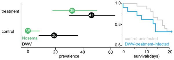
Prevalence of infections in treated Bombus terrestris workers 21 days after inoculation (in percent). Bars indicate 95% confidence intervals. Colours indicate treatment, with Nosema treated samples in green and DWV treated samples in black. Sample sizes are given inside the mean data point. The survival graph over the 21 day test period shows uninfected control treatments in grey compared to infected DWV treatments in blue (Cox mixed effects model fitted with penalized partial likelihood: X2 = 11.93, df = 4.17; p < 0.021, see Supplementary Information).
Having established both DWV and N. ceranae as infective for B. terrestris, we conducted a structured survey across 26 sites in GB and the Isle of Man, collecting 10 Apis samples, and 20 Bombus samples per site to assess EID prevalence (for details on the species identity across sites, see Extended Data Fig. 1). We analysed a total of 745 bees from 26 sites for DWV presence, DWV infection (replicating DWV) and N. ceranae presence. DWV was present in 20% (95% confidence interval (CI) 17-23%) of all samples; 36% (95% CI: 30-43%) of Apis and 11% (95% CI: 9-15%) of Bombus. Of the Apis harbouring DWV, 88% (95% CI: 70-98%) of the samples tested had actively replicating virus, whilst 38% (95% CI: 25-53%) of Bombus harbouring DWV had replicating virus (see Extended Data Fig. 2 and Extended Data Table 1). N. ceranae was less frequent, being detected in 7% (95% CI: 6-10%) of all samples; 9% (95% CI: 6-13%) of Apis samples and 7% (95% CI: 5-9%) of Bombus samples.
We estimated the GB-wide prevalence of the two pathogens in Apis and Bombus spp. based on our field survey data (Fig. 2). We found no evidence for spatial clustering of DWV presence in Bombus (Moran’s I = 0.023, p > 0.211) or either of the pathogens in Apis (DWV presence: Moran’s I = 0.03, p > 0.186; Nosema: Moran’s I = −0.061, p > 0.649). There was, however, weak clustering of DWV infection in Bombus (Moran’s I = 0.061, p < 0.044) and very strong clustering of N. ceranae in Bombus (Moran’s I = 0.25, p < 0.001), indicating disease hotspots for DWV in Bombus in the south west and east of GB and for N. ceranae in Bombus in the south east of GB (Fig. 2). Because prevalence was lower in Bombus than Apis, we modelled pathogen prevalence in Bombus as dependent on pathogen prevalence in Apis, Bombus to Apis density, and Apis abundance, including biologically relevant interactions whilst controlling for latitude, longitude, and sunlight hours, and adding collection site and species identity as random factors. Our full model for DWV presence was significantly better than the null model without any of the test predictors and their interactions included (likelihood ratio test: X2 = 19.03, df = 5, p < 0.002). After removal of the non-significant interactions (GLMM: Bombus to Apis density X DWV presence in Apis: estimate ± SE = −0.105 ± 1.376, p = 0.939; Apis abundance X DWV presence in Apis: 0.425 ± 1.309, p=0.745), it is clear that prevalence of DWV in Apis has a strong positive effect on DWV prevalence in Bombus (GLMM: 2.718 ± 0.921, z = 2.951, p < 0.004) (Fig. 2, Extended Data Fig. 3), while none of the other predictors played a role (GLMM: Bombus to Apis density: 0.315 ± 0.387, z = 0.814, p < 0.416; Apis abundance: −0.085 ± 0.364, z = −0.232, p < 0.816). In the case of N. ceranae, our full model was significantly better than the null model (X2 = 15.8, df = 5, p < 0.008). Specifically there was an effect of Nosema prevalence in Apis on Nosema prevalence in Bombus and this varied with Apis abundance (interaction between Nosema prevalence in Apis and Apis abundance: X2 = 7.835, df = 2, p < 0.02), while Bombus to Apis density did not explain Nosema prevalence in Bombus (GLMM: 8.386 ± 6.793, z = 1.235, p = 0.217) (Fig. 2, Extended Data Fig. 3).
Figure 2. Prevalence.

Estimated pathogen prevalence in Apis and Bombus across Great Britain and the Isle of Man. Colour gradient (based on Gaussian kernel estimators with an adaptive bandwidth of equal number of observations over 26 sites, see Methods) corresponds to percent prevalence (note different scales). DWV prevalence is displayed in blue and Nosema prevalence in green.
The prevalence data implied local transmission of DWV between Apis and Bombus. To test this, we sequenced up to 5 isolates per DWV infected Bombus sample from 5 sites matched by up to 5 isolates of sympatric DWV infected Apis samples. If a pathogen is transmitted between these two hosts, we would expect Apis and Bombus to share the same DWV strain variants within a site. Marginal log likelihoods estimated by stepping stone sampling23 decisively support clades constrained by site as opposed to host, indicating pathogen transmission within site (Fig. 3, Extended Data Table 2).
Figure 3. Viral strain relations.

RNA-dependent RNA polymerase (RdRp) partial gene phylogeny of pollinator viruses (main text). Gene trees were estimated using PhyML v.3.0 maximum-likelihood (ML) bootstrapping (500 replicates) and MrBayes v3.1.2 (see Methods). Coloured boxes correspond to sites H, L, Q, R and X (as shown on the map) while text colours correspond to host (Red: Bombus; Black: Apis). Symbols represent node support values: posterior probability (left), bootstrap support (right). Filled circle: >90%, Target symbol: >70%, Empty circle: >50%. Branches (//) one third of true length.
Our results provide evidence for an emerging pathogen problem in wild pollinators that may be driven by Apis. Our data cannot demonstrate directionality in the interspecific transmission of DWV. However, the high prevalence of DWV in honey bees, which is a consequence of the exotic vector Varroa destructor24, is consistent with their acting as the major source of infection for the pollinator community. Similar results have been found for intraspecific transmission of Bombus-specific pathogens from high prevalence commercial Bombus colonies to low prevalence wild Bombus populations18. Our field estimates of prevalence are conservative for DWV, as highly infected individuals have deformed wings, are incapable of flight, and thus would not be captured by our sampling protocol. Consequently, DWV prevalence and, as a result, impact are likely to be higher in managed and wild populations than our data suggest. Interestingly, N. ceranae prevalence in Bombus depends positively on Apis abundance, but only when N. ceranae prevalence in Apis is low, suggesting a possible environmental saturation effect of N. ceranae spores. In contrast to the low impact of N. ceranae on the survival of B. terrestris in our study, Graystock et al.25 found very high virulence. This might be explained by our use of young bees vs Graystock et al.’s25 non-age-controlled design, indicating age dependent differential susceptibility in B. terrestris, as has been shown to be the case in honey bees26.
Ongoing spillover of EIDs could represent a major cause of mortality of wild pollinators wherever managed bees are maintained. While our data are only drawn from GB, the prerequisites for honey bees to be a source or reservoir for these EIDs – high colony densities and high parasite loads – are present at a global scale. In addition, global trade in both honey bees and commercial Bombus may exacerbate this impact6,27. Reducing the pathogen burden in managed honey bees so as to reduce the risk of transmission to wild pollinators is not straightforward. Tighter control of importation and hygiene levels of transported colonies could be imposed with regulation, but policies developed in this direction must learn from the past; such regulation is difficult to implement and hard to evaluate9,28. Clearly, it is essential to ensure that those managing bees (including commercial producers, growers and beekeepers) have access to the methods and skills to monitor, manage and control EIDs for the benefit of their managed colonies, and the wider pollinator community. A consensus on the threat of EIDs for wild pollinators can only be reached with greater knowledge of their epidemiology, global extent and impact, and it will be crucial to involve key stakeholders (e.g. the beekeeping community, Bombus exporters) in any decision process, as any progress made will largely be driven by their actions.
Methods
Bombus inoculation experiment
Each of the 7 experimental Bombus terrestris colonies (Biobest) was tested for presence of the two treatment pathogens DWV and N. ceranae. Daily, callows (newly emerged workers) were removed from the colony, assigned sequentially to random treatment blocks and housed individually in small Perspex boxes on an ad libitum diet of 50% sucrose solution and artificial pollen (Nektapoll), as natural pollen has been shown to contain viable N. ceranae spores and DWV virions 19,37. Two day old bumble bee workers were individually inoculated with a treatment dependent inoculum in 10 μl sucrose. Crude hindgut extracts of 5 Apis workers propagating N. ceranae were purified by the triangulation method38 with slight adaptations.
We used small cages with 30 N. ceranae infected honey bees to propagate N. ceranae spores for the inoculum. Every second day we collected 5 honey bees from these cages, and removed and ground the hindguts. The resulting extract was filtered through cotton and washed with 0.9% insect ringer (Sigma Aldrich). We triangulated extracts using Eppendorf tubes and spin speeds of 0.5g for 3 minutes, purifying N. ceranae spores over 7 tubes. Spore numbers were quantified in a Neubauer counting chamber. In parallel, we extracted and purified N. ceranae free bees to use for control inoculations.
DWV virus inoculum was prepared according to Bailey & Ball39 with modifications. Honeybees with DWV symptoms (crippled wings and body deformities) were crushed in 0.5M potassium phosphate buffer (pH 8.0), filtered and clarified by slow speed centrifugation (8000g for 10 minutes) before being diluted and injected (1μl) into white-eyed pupae for bulk propagation of virus. After 5 days, up to 100 pupae were harvested, and after a further screen by qRT-PCR, virus was purified as follows. Virus extraction buffer consisted of 0.5M potassium phosphate pH 8.0, 0.2% DEICA, 10% diethyl ether. Purification consisted of two slow speed clarifications (8000g for 10 minutes), one high speed clarification (75000g for 3 hours) followed by re-suspension in 0.5M potassium phosphate buffer (ph8.0) and a final slow speed clarification. Virus preparations were aliquoted and stored at −80°C until use in inoculation experiments.
The purified virus was checked by quantitative Reverse Transcription (qRT) PCR for the presence of DWV and the absence of other common honey bee RNA viruses: BQCV, IAPV, SBV, CBPV, ABPV, and SBPV by PCR.
A duplicate dilution series of external DNA standards covering 102 to 108 molecules (reaction efficiencies: 90-110%, r2: 0.95-0.99) were included in qRT-PCR runs to quantify DWV genome equivalents present in the inoculum. For absolute quantification of virus dose, an external DNA standard was generated by amplifying a genomic fragment of 241bp using the primers F8668std (5′-GAT GGG TTT GAT TCG ATA TCT TGG-3′) and B8757std (5′-GGC AAA CAA GTA TCT TTC AAA CAA TC-3′) via RT-PCR that contained the 136bp fragment amplified by the DWV-specific qRT-PCR primers F8668/B875740.
Shortly before administering, inocula were prepared to a total concentration of 105 spores/bee in 10 μl (104 spores/μl sucrose solution). Inocula were administered individually in a small Petri dish after 30-60 minutes starvation. Only workers ingesting the full 10 μl within 1h were used in the experiment.
Sampling scheme
The mainland sampling sites were chosen across Great Britain along a north-south transect (12 sampling points with fixed latitude, but free in longitude) and across two east-west transects (12 sampling points with fixed longitude, but free within a narrow latitudinal corridor). Each of the mainland sites were at least 30 km apart (mean ± SD of nearest neighbour = 69.21 ± 26.39). The island sites were chosen deliberately to gain background data for both Apis and Bombus disease prevalence in the absence of Varroa, the main transmission route for DWV in Apis. At each sampling site we collected approximately 30 workers for each of the following species: Apis mellifera, Bombus terrestris (verified by RFLP-analysis29), and the next most common bumble bee on site. We collected free flying bees from flowers rather than bees from colonies as this is the most likely point of contact in the field. By collecting from flowers we lowered the likelihood of collecting bumblebees from different colonies. While we ran the risk of collecting multiple honeybees from the same hive, this nevertheless represents the potential force of infection for both genera in the field.
Each collection took place along a continuous transect, where maximally ten bees per ten metre stretch were collected before moving on to the next ten metre stretch. At each site, the collection area covered at least 1000 m2 (e.g., 10 × 100m, 20 × 50m). Each sampling point was within one of the following landcover types: urban areas (gardens and parks), farmland (hedgerows, border strips, crops, and wildflower meadows), coastal cliffs, sand dunes and heather moorland.
If possible, we collected all bees within a single day. In the case of adverse weather, we returned as soon as possible to finish the collection at the exact same site. To estimate Apis and Bombus densities at each site we timed the collection effort simultaneously. Time taken to collect 20 Bombus workers (of any Bombus species) and 20 Apis workers was recorded, respectively. Timed collecting efforts took place on a single day only.
Samples collected were put in sampling tubes, transferred straight onto ice, then freeze-killed at −20°C and transferred to −80°C as soon as possible thereafter to ensure optimal RNA (DWV) preservation.
RNA work
RNA extraction followed the standard RNeasy plant mini kit (Qiagen) protocol with the final elutate (in RNase free ddH2O) of 30 μl being run over the column twice (for optimal RNA concentration). For reverse transcription of RNA to cDNA we followed the standard protocol of the Nanoscript Kit (Primerdesign). Our priming was target specific in separate reactions for N. ceranae (primer pair N. ceranae41), DWV (primer pair F15/B2342) and a housekeeping gene (primer pair ACTB43) as a positive control for RNA extraction efficiency. Bees were transferred to liquid N2 prior to dissection. Each bee’s abdomen was cut with a sterile scalpel dorsoventrally along the sagittal plane. One half was submerged in RLT buffer (Qiagen) for RNA extraction, and the second half was archived at −80C. Tissue disruption and homogenisation of individual half-abdomens was performed on a tissue lyser II (Qiagen) at 30Hz for 2 minutes followed by 20Hz for 2 minutes. RNA quality and quantity were checked on a Spectrometer (Nanodrop, Thermo Scientific). cDNA preparation was conducted at 65°C for 5 minutes for the initial priming immediately before the addition of the reverse transcriptase. For the extension, samples were incubated at 25°C for 5 minutes followed by 55 °C for 20 minutes and then heat inactivated for 15 minutes at 75°C. cDNA was used as template in a standard PCR with 57°C, 54°C, and 57°C annealing temperatures, respectively. Results were visualized on a 2% agarose gel with EtBr under UV light. Agarose gels were scored without knowledge of sample ID. To verify the specificity of the amplicon, one purified PCR product taken from Apis and one taken from B. lapidarius were sequenced (Macrogen Inc.).
Detection of negative strand DWV
Detection of pathogens in pollinators in the field does not provide proof of infection, as pathogens are likely being ingested on shared, contaminated food resources and therefore are inevitably present in the gut-lumen as passive contaminants without necessarily infecting the host. To minimize these cases, we tested all our DWV positive Bombus samples and a subset of DWV positive Apis samples for virus replication, a strong indicator for infection44. DWV is a positive strand virus whose negative strand is only present in a host once the virus is actively replicating39. Reverse transcription was conducted using a tagged primer tagB2345 for the initial priming to target exclusively the negative strand. The resulting cDNA was used in a PCR with the tag sequence and F15 as primers30,45. We tested all Bombus samples that were positive for DWV presence and, where possible, 2 DWV-positive Apis samples from each site where we found DWV in Bombus.
Sequencing
DWV sequence diversity was analysed by sequencing up to 5 independent clones per DWV negative-strand infected Bombus sample from 5 sites (H, L, Q, R, X; chosen for their high DWV infected prevalence in Bombus) and 5 clones of DWV infected Apis samples from the same sites (we checked extra Apis samples for DWV infection if necessary to match Bombus DWV infections). All Bombus samples were B. lapidarius with the exception of one sample from site L (clone05), which was B. pascuorum (this sample is not included in any of the other analyses, but revealed a DWV infection in an initial screening and was hence included in the virus variant analysis). We sequenced a region of the DWV genome: the RNA-dependent RNA polymerase (RdRp) gene (F15/B23 primer pair42 used throughout the study). RdRp is thought to be a conserved region of the virus genome where non-synonymous substitutions may have significant implications for the epidemiology of the virus 24. RT-PCRs and PCR were run as described before. DWV PCR products were verified by gel electrophoresis as described above; if a clear, clean single band was visible, we proceeded directly to the cloning protocol. If not, we purified products from the agarose gel following a standard protocol (Qiaquick Gel Extraction Kit, Qiagen) and used the purified fragment in an additional PCR. PCR products were cloned using the Invitrogen TA cloning kit (Invitrogen), according to the manufacturer’s instructions. Plasmid DNA was isolated using the Spin Miniprep kit (Qiagen) and the successful insertion of target sequence was tested by restriction analysis (digested with EcoR I). Up to 5 clones per sample were sequenced in forward and reverse orientation (Source BioSciences, Cambridge).
Analysis of DWV sequences
The 75 Apis and Bombus clones from sites H, L, Q, R and X were supplemented with DWV and VDV reference RdRp sequences (accession nos. NC004830 and NC006494 respectively), resulting in a final alignment of 420bp from 77 sequences. Forward and reverse sequences of each clone were assembled and the consensus sequence was used for further analysis. Sequences were aligned using Geneious (R 6.1.6) with standard settings. Ends were trimmed by hand. For the tree building we conducted two independent (MC)3 algorithms running for 2 million generations, each with four chains (3 hot, 1 cold), sampling one tree in 1000, under the GTR+Ґ (nst = 6) substitution model. Gene trees were estimated using PhyML v.3.046 maximum-likelihood (ML) bootstrapping (500 replicates) and MrBayes v3.1.247, under a GTR model of sequence evolution and a gamma (Ґ) model, using 4 categories to accommodate rate variation across sites. Burn-in cutoffs were inspected manually for each parameter file in Tracer v1.448. Inspection of the standard deviation of split frequencies confirmed that runs had converged (0.0093). To test alternative a priori hypotheses of virus diversification, for each virus (DWV and VDV) we constrained clades according to site (H, L, Q, R and X) or host genus (Apis and Bombus), and performed stepping stone sampling23 as implemented in MrBayes v3.1.2 to accurately estimate marginal log likelihoods. MCMC sampling was conducted for 50 steps of 39000 generations each, with the first 9000 generations of every step discarded as burn-in. The model with the highest likelihood score was used as the null hypothesis. We compared Bayes Factors (BF) for both models and used a threshold of 2 ln (BF) > 10 as decisive support for the null against the alternative hypothesis49 (Supplementary Table 2). We repeated stepping stone sampling to confirm run stability (data not shown).
Statistics
Mean survival of control treatments, free of the two test pathogens, was 14.2 ± 4.2 (mean ± sd) days, while DWV treated bees survived for 8.1 ± 5.8 (mean ± sd) days. To assess the effect of infection on survival we fitted a Cox mixed effects model with treatment as a fixed factor and colony origin as random factor and compared it to the null model 50(R library coxme, version 2.2-3, function coxme). The model was fitted with the penalized partial likelihood (PPL) and showed a significant negative impact of infection on longevity (X2 = 11.93, df = 4.17; p < 0.021).
N. ceranae treated bees survived for 18 ± 1 (mean ± sd) days. A model with treatment as fixed factor and colony origin as random factor showed no improvement over the null model (PPL: X2 = 0.12, df = 1; p > 0.735).
True prevalences with 95% confidence intervals were computed to correct for varying sample sizes (due to the different species of bumble bee at the sampling sites) and test sensitivity was set to a conservative 95% 51. Confidence interval estimates are based on Blaker’s (2000) method for exact two sided confidence intervals 52 for each sampling site and for each species sampled 31(R library epiR, version 0.9-45, function epi.prev).
To investigate our spatially distributed dataset we undertook an exploratory data analysis (EDA)53 in which we calculated a prevalence surface for each of our parasites using Gaussian kernel estimators with an adaptive bandwidth of equal number of observations. This is a variant of the nearest neighbour technique, with bandwidth size being determined by a minimum number of observations in the neighbourhood (set to 3 times the maximum observations per site)32 (R library prevR, version 2.1, function kde). Estimated surfaces were used for visual inspection only (Fig. 2); all the remaining analyses are based on the raw data only.
To investigate spatial structure and disease hotspots we used spatial autocorrelation statistics of the true prevalence of each of the pathogens in the different host genera from the 26 collection sites. To identify whether or not the pathogens we found were spatially clustered, we computed the spatial autocorrelation coefficient Moran’s I54 with an inverse spatial distance weights matrix, as implemented in Gittleman and Kot 55 (R library ape, version 3.0-7, function Moran.I). Moran’s I is a weighted measure describing the relationship of the prevalence values associated with spatial points. The coefficient ranges from −1 (perfect dispersion) through 0 (no spatial autocorrelation (random distribution)) to 1 (perfect clustering).
To investigate whether pathogen prevalence (Nosema and DWV were tested in separate models) in Apis, Bombus to Apis relative density, or Apis absolute abundance had an effect on pathogen prevalence in Bombus, we ran a Generalized Linear Mixed Model (GLMM) 34 with binomial error structure and logit link function using the function lmer of the R package lme435. Latitude, longitude, sunlight hours (a proxy for favourable foraging weather that would enable disease transmission; calculated cumulatively from March until the month of collection [data were collected from the MET office webpage: http://www.metoffice.gov.uk/climate/uk/anomacts/, averaging over area sunlight hour ranges]) and landcover type were included in the model as fixed control effects (present in the full as well as the null model) while site and species were included in the model as random effects (present in the full as well as the null model). Before running the model we inspected all predictors for their distribution, as a consequence of which we log transformed “Bombus to Apis density” and “Apis abundance” to provide more symmetrical distributions. Thereafter we z-transformed all quantitative predictors to a mean of zero and a standard deviation of one to derive more comparable estimates and to aid interpretation of interactions56. Since changes in “Bombus to Apis density” and “Apis abundance” could lead to changes in pathogen prevalence in Bombus because of a change in pathogen prevalence in Apis, we included the interactions between “Bombus to Apis density” and pathogen prevalence in Apis, and “Apis abundance” and pathogen prevalence in Apis. To test the overall effect of our three test predictors, we compared the full model with a reduced model (null model) using a likelihood ratio test comprising latitude, longitude, sunlight hours and landcover type with the same random effects structure. Model stability was assessed by excluding data points one by one and comparing the estimates derived from these reduced models with estimates from the full model (revealing a stable model). Site G had to be excluded from this analysis as no Apis samples were found on site.
We fitted linear models to assess the relationships of parasite prevalence among Apis and Bombus.
We investigated the effect of pathogen treatment on disease status of an individual with a Generalized Linear Mixed Model (GLMM) 34) with binomial error structure and logit link function using the function lmer of the R package lme435. Colony of origin was entered into the model as a random effect. As described before, we checked model stability (the model with interaction terms included was unstable; however it stabilised once the non-significant interaction terms were removed), before testing the full model against the null model using a likelihood ratio test. All analyses were run in R36.
Supplementary Material
Distribution of sampling sites across Great Britain and the Isle of Man. The most common Bombus species on site is represented by coloured letters while the 2nd most common Bombus species is represented by differently coloured dots. Total sample sizes for each site are given in the table.
Pathogen prevalence in Bombus spp. in percent per site (a. for DWV; b. for N. ceranae) and per species (c. for DWV; d. for N. ceranae). Bars indicate 95% confidence intervals. Note different scales
The linear models shown only illustrate the relationships but do not drive the conclusions in the main text. a) DWV presence in Apis and Bombus (adj R2 = 0.34, p < 0.001); b) DWV replicating in Bombus and DWV presence in Bombus (adj R2 = 0.46, p < 0.001); c) N. ceranae presence in Apis and Bombus (adj R2 = −0.04, p > 0.728). The line shows the best fit and the dark grey region shows 95%CI of fit.
Pathogen prevalence is given in percent with 95% confidence intervals (% prevalence [95% CI]). Sample numbers (N) are shown in brackets.
Footnote to Extended Data Table 1: * out of the 31 DWV present Apis samples tested
Acknowledgments
We are grateful to E. Fürst for technical support and R.J. Gill for discussions. We thank C. Jones, G. Baron, O. Ramos-Rodriguez for comments on previous versions of the manuscript. Thanks to Hymettus Ltd. for help with the field collections, K. Liu for help in the laboratory and B. McCrea and S. Baldwin for technical help in the bee-laboratory. The study was supported by the Insect Pollinator Initiative (funded jointly by the Biotechnology and Biological Sciences Research Council, the Department for Environment, Food and Rural Affairs, the Natural Environment Research Council, The Scottish Government and The Wellcome Trust, under the Living with Environmental Change Partnership: grant BB/I000151/1 (M.J.F.B.), BB/I000100/1 (R.J.P.), BB/I000097/1 (J.O.)).
References
- 1.Binder S, Levitt AM, Sacks JJ, Hughes JM. Emerging infectious diseases: public health issues for the 21st century. Science. 1999;284:1311–1313. doi: 10.1126/science.284.5418.1311. doi: 10.1126/science.284.5418.1311. [DOI] [PubMed] [Google Scholar]
- 2.Oldroyd BP. Coevolution while you wait: Varroa jacobsoni, a new parasite of western honeybees. Trends Ecol. Evol. 1999;14:312–315. doi: 10.1016/s0169-5347(99)01613-4. doi: 10.1016/S0169-5347(99)01613-4. [DOI] [PubMed] [Google Scholar]
- 3.Ratnieks FLW, Carreck NL. Clarity on honey bee collapse? Science. 2010;327:152–153. doi: 10.1126/science.1185563. doi: 10.1126/science.1185563. [DOI] [PubMed] [Google Scholar]
- 4.Vanbergen AJ, The Insect Pollinator Initiative. Threats to an ecosystem service: pressures on pollinators. Front. Ecol. Environ. 2013;11:251–259. doi: 10.1890/120126. [Google Scholar]
- 5.Williams PH, Osborne JL. Bumblebee vulnerability and conservation world-wide. Apidologie. 2009;40:367–387. doi: 10.1051/apido/2009025. [Google Scholar]
- 6.Cameron SA, et al. Patterns of widespread decline in North American bumble bees. Proc. Natl. Acad. Sci. U. S. A. 2011;108:662–667. doi: 10.1073/pnas.1014743108. doi: 10.1073/pnas.1014743108. [DOI] [PMC free article] [PubMed] [Google Scholar]
- 7.Evison SEF, et al. Pervasiveness of parasites in pollinators. PLoS ONE. 2012;7 doi: 10.1371/journal.pone.0030641. doi: ARTNe30641DOI10.1371/journal.pone.0030641. [DOI] [PMC free article] [PubMed] [Google Scholar]
- 8.Genersch E, Yue C, Fries I, de Miranda JR. Detection of deformed wing virus, a honey bee viral pathogen, in bumble bees (Bombus terrestris and Bombus pascuorum) with wing deformities. J. Invertebr. Pathol. 2006;91:61–63. doi: 10.1016/j.jip.2005.10.002. doi: 10.1016/j.jip.2005.10.002. [DOI] [PubMed] [Google Scholar]
- 9.Meeus I, Brown MJF, De Graaf DC, Smagghe G. Effects of invasive parasites on bumble bee declines. Conserv. Biol. 2011;25:662–671. doi: 10.1111/j.1523-1739.2011.01707.x. doi: 10.1111/j.1523-1739.2011.01707.x. [DOI] [PubMed] [Google Scholar]
- 10.Fisher MC, et al. Emerging fungal threats to animal, plant and ecosystem health. Nature. 2012;484:186–194. doi: 10.1038/nature10947. doi: 10.1038/Nature10947. [DOI] [PMC free article] [PubMed] [Google Scholar]
- 11.Krebs J, et al. Bovine tuberculosis in cattle and badgers. MAFF Publications; 1997. [Google Scholar]
- 12.Vitousek PM, Dantonio CM, Loope LL, Westbrooks R. Biological invasions as global environmental change. Am. Sci. 1996;84:468–478. [Google Scholar]
- 13.Daszak P. Emerging infectious diseases of wildlife - Threats to biodiversity and human health. Science. 2000;287:443–9. doi: 10.1126/science.287.5452.443. [DOI] [PubMed] [Google Scholar]
- 14.Dobson A. Population dynamics of pathogens with multiple host species. Am. Nat. 2004;164:S64–S78. doi: 10.1086/424681. doi: 10.1086/424681. [DOI] [PubMed] [Google Scholar]
- 15.Alderman DJ. Geographical spread of bacterial and fungal diseases of crustaceans. Rev. Sci. Tech. 1996;15:603–632. doi: 10.20506/rst.15.2.943. [DOI] [PubMed] [Google Scholar]
- 16.Neumann P, Carreck NL. Honey bee colony losses. J. Apic. Res. 2010;49:1–6. doi: 10.3896/Ibra.1.49.1.01. [Google Scholar]
- 17.Paxton RJ. Does infection by Nosema ceranae cause “Colony Collapse Disorder” in honey bees (Apis mellifera)? J. Apic. Res. 2010;49:80–84. doi: 10.3896/Ibra.1.49.1.11. [Google Scholar]
- 18.Murray TE, Coffey MF, Kehoe E, Horgan FG. Pathogen prevalence in commercially reared bumble bees and evidence of spillover in conspecific populations. Biol. Conserv. 2013;159:269–276. doi: 10.1016/j.biocon.2012.10.021. doi: 10.1016/j.biocon.2012.10.021. [DOI] [PMC free article] [PubMed] [Google Scholar]
- 19.Singh R, et al. RNA viruses in Hymenopteran pollinators: evidence of inter-taxa virus tansmission via pollen and potential impact on non-Apis Hymenopteran species. PLoS ONE. 2010;5:e14357. doi: 10.1371/journal.pone.0014357. doi: 10.1371/journal.pone.0014357. [DOI] [PMC free article] [PubMed] [Google Scholar]
- 20.Graystock P, et al. The Trojan hives: pollinator pathogens, imported and distributed in bumblebee colonies. J. Appl. Ecol. 2013;50:1207–1215. doi: 10.1111/1365-2664.12134. [Google Scholar]
- 21.Ongus JR, et al. Complete sequence of a picorna-like virus of the genus Iflavirus replicating in the mite Varroa destructor. J. Gen. Virol. 2004;85:3747–3755. doi: 10.1099/vir.0.80470-0. doi: 10.1099/vir.0.80470-0. [DOI] [PubMed] [Google Scholar]
- 22.Moore J, et al. Recombinants between deformed wing virus and Varroa destructor virus-1 may prevail in Varroa destructor-infested honeybee colonies. J. Gen. Virol. 2011;92:156–161. doi: 10.1099/vir.0.025965-0. doi: 10.1099/Vir.0.025965-0. [DOI] [PubMed] [Google Scholar]
- 23.Xie W, Lewis PO, Fan Y, Kuo L, Chen M-H. Improving marginal likelihood estimation for bayesian phylogenetic model selection. Syst. Biol. 2011;60:150–160. doi: 10.1093/sysbio/syq085. doi: 10.1093/sysbio/syq085. [DOI] [PMC free article] [PubMed] [Google Scholar]
- 24.Martin SJ, et al. Global honey bee viral landscape altered by a parasitic mite. Science. 2012;336:1304–1306. doi: 10.1126/science.1220941. doi: 10.1126/science.1220941. [DOI] [PubMed] [Google Scholar]
- 25.Graystock P, Yates K, Darvill B, Goulson D, Hughes WOH. Emerging dangers: deadly effects of an emergent parasite in a new pollinator host. J. Invertebr. Pathol. 2013 doi: 10.1016/j.jip.2013.06.005. doi: 10.1016/j.jip.2013.06.005. [DOI] [PubMed] [Google Scholar]
- 26.Smart MD, Sheppard WS. Nosema ceranae in age cohorts of the western honey bee (Apis mellifera) J. Invertebr. Pathol. 2012;109:148–151. doi: 10.1016/j.jip.2011.09.009. doi: 10.1016/j.jip.2011.09.009. [DOI] [PubMed] [Google Scholar]
- 27.Otterstatter MC, Thomson JD. Does pathogen spillover from commercially reared bumble bees threaten wild pollinators? PLoS ONE. 2008;3 doi: 10.1371/journal.pone.0002771. doi: 10.1371/Journal.Pone.0002771. [DOI] [PMC free article] [PubMed] [Google Scholar]
- 28.Donnelly CA, Woodroffe R. Reduce uncertainty in UK badger culling. Nature. 2012;485:582–582. doi: 10.1038/485582a. [DOI] [PubMed] [Google Scholar]
- 29.Murray TE, Fitzpatrick U, Brown MJF, Paxton RJ. Cryptic species diversity in a widespread bumble bee complex revealed using mitochondrial DNA RFLPs. Conserv. Genet. 2008;9:653–666. doi: 10.1007/s10592-007-9394-z. [Google Scholar]
- 30.Craggs JK, Ball JK, Thomson BJ, Irving WL, Grabowska AM. Development of a strand-specific RT-PCR based assay to detect the replicative form of hepatitis C virus RNA. J. Virol. Methods. 2001;94:111–120. doi: 10.1016/s0166-0934(01)00281-6. doi: 10.1016/S0166-0934(01)00281-6. [DOI] [PubMed] [Google Scholar]
- 31.epiR: an R package for the analysis of epidemiological data. (Version 0.9-45) 2012
- 32.Larmarange J, Vallo R, Yaro S, Msellati P, Meda N. Methods for mapping regional trends of HIV prevalence from demographic and health surveys (DHS) Cybergeo: Europ. J. Geo. 2011;558 doi: 10.4000/cybergeo.24606. [Google Scholar]
- 33.Paradis E, Claude J, Strimmer K. APE: Analyses of phylogenetics and evolution in R language. Bioinformatics. 2004;20:289–290. doi: 10.1093/bioinformatics/btg412. doi: 10.1093/bioinformatics/btg412. [DOI] [PubMed] [Google Scholar]
- 34.Baayen RH, Davidson DJ, Bates DM. Mixed-effects modeling with crossed random effects for subjects and items. J. Mem. Lang. 2008;59:390–412. doi: 10.1016/j.jml.2007.12.005. [Google Scholar]
- 35.Bates D, Maechler M, Bolker B. lme4: Linear mixed-effects models using S4 classes. 2012. [Google Scholar]
- 36.R: a language and environment for statistical computing. R Foundation for Statistical Computing; Vienna, Austria: 2012. [Google Scholar]
- 37.Higes M, Martin-Hernandez R, Garrido-Bailon E, Garcia-Palencia P, Meana A. Detection of infective Nosema ceranae (Microsporidia) spores in corbicular pollen of forager honeybees. J. Invertebr. Pathol. 2008;97:76–78. doi: 10.1016/j.jip.2007.06.002. doi: 10.1016/j.jip.2007.06.002. [DOI] [PubMed] [Google Scholar]
- 38.Cole RJ. Application of triangulation method to purification of Nosema spores from insect tissues. J. Invertebr. Pathol. 1970;15:193–&. [Google Scholar]
- 39.Bailey LL, Ball BV. Honey bee pathology. 2nd edn Academic Press; 1991. [Google Scholar]
- 40.Yanez O, et al. Deformed wing virus and drone mating flights in the honey bee (Apis mellifera): implications for sexual transmission of a major honey bee virus. Apidologie. 2012;43:17–30. doi: 10.1007/s13592-011-0088-7. [Google Scholar]
- 41.Chen Y, Evans JD, Smith IB, Pettis JS. Nosema ceranae is a long-present and widespread microsporidian infection of the European honey bee (Apis mellifera) in the United States. J. Invertebr. Pathol. 2008;97:186–188. doi: 10.1016/j.jip.2007.07.010. doi: 10.1016/j.jip.2007.07.010. [DOI] [PubMed] [Google Scholar]
- 42.Genersch E. Development of a rapid and sensitive RT-PCR method for the detection of deformed wing virus, a pathogen of the honeybee (Apis mellifera) Vet. J. 2005;169:121–123. doi: 10.1016/j.tvjl.2004.01.004. doi: 10.1016/j.tvjil.2004.01.004. [DOI] [PubMed] [Google Scholar]
- 43.Hornakova D, Matouskova P, Kindl J, Valterova I, Pichova I. Selection of reference genes for real-time polymerase chain reaction analysis in tissues from Bombus terrestris and Bombus lucorum of different ages. Anal. Biochem. 2010;397:118–120. doi: 10.1016/j.ab.2009.09.019. doi: 10.1016/J.Ab.2009.09.019. [DOI] [PubMed] [Google Scholar]
- 44.de Miranda JR, Genersch E. Deformed wing virus. J. Invertebr. Pathol. 2010;103:S48–S61. doi: 10.1016/j.jip.2009.06.012. doi: 10.1016/j.jip.2009.06.012. [DOI] [PubMed] [Google Scholar]
- 45.Yue C, Genersch E. RT-PCR analysis of deformed wing virus in honeybees (Apis mellifera) and mites (Varroa destructor) J. Gen. Virol. 2005;86:3419–3424. doi: 10.1099/vir.0.81401-0. doi: 10.1099/vir.0.81401-0. [DOI] [PubMed] [Google Scholar]
- 46.Guindon S, et al. New algorithms and methods to estimate maximum-likelihood phylogenies: assessing the performance of PhyML 3.0. Syst. Biol. 2010;59:307–321. doi: 10.1093/sysbio/syq010. doi: 10.1093/sysbio/syq010. [DOI] [PubMed] [Google Scholar]
- 47.Huelsenbeck JP, Ronquist F. MRBAYES: Bayesian inference of phylogenetic trees. Bioinformatics. 2001;17:754–755. doi: 10.1093/bioinformatics/17.8.754. doi: 10.1093/bioinformatics/17.8.754. [DOI] [PubMed] [Google Scholar]
- 48.Tracer v1.4. 2007 Available at: http://beast.bio.ed.ac.uk/Tracer.
- 49.de Bruyn M, et al. Paleo-drainage basin connectivity predicts evolutionary relationships across three southeast Asian biodiversity hotspots. Syst. Biol. 2013;62:398–410. doi: 10.1093/sysbio/syt007. doi: 10.1093/sysbio/syt007. [DOI] [PubMed] [Google Scholar]
- 50.coxme: Mixed Effects Cox Models. 2012 Available at: http://CRAN.R-project.org/package=coxme.
- 51.Reiczigel J, Foldi J, Ozsvari L. Exact confidence limits for prevalence of a disease with an imperfect diagnostic test. Epidemiol. Infect. 2010;138:1674–1678. doi: 10.1017/S0950268810000385. doi: 10.1017/S0950268810000385. [DOI] [PubMed] [Google Scholar]
- 52.Blaker H. Confidence curves and improved exact confidence intervals for discrete distributions. Canadian Journal of Statistics-Revue Canadienne De Statistique. 2000;28:783–798. doi: 10.2307/3315916. [Google Scholar]
- 53.Rossi RE, Mulla DJ, Journel AG, Franz EH. Geostatistical tools for modeling and interpreting ecological spatial dependence. Ecol. Monogr. 1992;62:277–314. doi: 10.2307/2937096. [Google Scholar]
- 54.Moran PA. Notes on continuous stochastic phenomena. Biometrika. 1950;37:17–23. [PubMed] [Google Scholar]
- 55.Gittleman JL, Kot M. Adaptation - statistics and a null model for estimating phylogenetic effects. Syst. Zool. 1990;39:227–241. doi: 10.2307/2992183. [Google Scholar]
- 56.Schielzeth H. Simple means to improve the interpretability of regression coefficients. Meth. Ecol. Evol. 2010;1:103–113. doi: 10.1111/j.2041-210X.2010.00012.x. [Google Scholar]
Associated Data
This section collects any data citations, data availability statements, or supplementary materials included in this article.
Supplementary Materials
Distribution of sampling sites across Great Britain and the Isle of Man. The most common Bombus species on site is represented by coloured letters while the 2nd most common Bombus species is represented by differently coloured dots. Total sample sizes for each site are given in the table.
Pathogen prevalence in Bombus spp. in percent per site (a. for DWV; b. for N. ceranae) and per species (c. for DWV; d. for N. ceranae). Bars indicate 95% confidence intervals. Note different scales
The linear models shown only illustrate the relationships but do not drive the conclusions in the main text. a) DWV presence in Apis and Bombus (adj R2 = 0.34, p < 0.001); b) DWV replicating in Bombus and DWV presence in Bombus (adj R2 = 0.46, p < 0.001); c) N. ceranae presence in Apis and Bombus (adj R2 = −0.04, p > 0.728). The line shows the best fit and the dark grey region shows 95%CI of fit.
Pathogen prevalence is given in percent with 95% confidence intervals (% prevalence [95% CI]). Sample numbers (N) are shown in brackets.
Footnote to Extended Data Table 1: * out of the 31 DWV present Apis samples tested