Posterior Predictive Bayesian Phylogenetic Model Selection

Abstract

We present two distinctly different posterior predictive approaches to Bayesian phylogenetic model selection and illustrate these methods using examples from green algal protein-coding cpDNA sequences and flowering plant rDNA sequences. The Gelfand–Ghosh (GG) approach allows dissection of an overall measure of model fit into components due to posterior predictive variance (GG_p) and goodness-of-fit (GG_g), which distinguishes this method from the posterior predictive P-value approach. The conditional predictive ordinate (CPO) method provides a site-specific measure of model fit useful for exploratory analyses and can be combined over sites yielding the log pseudomarginal likelihood (LPML) which is useful as an overall measure of model fit. CPO provides a useful cross-validation approach that is computationally efficient, requiring only a sample from the posterior distribution (no additional simulation is required). Both GG and CPO add new perspectives to Bayesian phylogenetic model selection based on the predictive abilities of models and complement the perspective provided by the marginal likelihood (including Bayes Factor comparisons) based solely on the fit of competing models to observed data. [Bayesian; conditional predictive ordinate; CPO; L-measure; LPML; model selection; phylogenetics; posterior predictive.]

Criticizing the model used is an important step in phylogenetic analyses (Sullivan and Joyce 2005; Ripplinger and Sullivan 2010). Many Bayesian phylogenetic analyses use ModelTest (Posada and Crandall 1998), MrModelTest (Nylander 2008), or JModelTest (Posada 2008) software to choose the model. These programs use output from PAUP* (Swofford 2002) or PhyML (Guindon et al. 2010) to perform likelihood ratio tests (LRTs; Wilks 1938), or compute the Akaike information criterion (AIC; Akaike 1974) or the Bayesian information criterion (BIC; Schwarz 1978) in order to rank models. Although practical, this approach is less than ideal because LRTs, AIC, and BIC all judge a model solely on how it performs at its best (the maximum likelihood point), ignoring the prior distribution, which is an important component of any Bayesian model. The marginal likelihood provides an alternative to AIC and BIC that correctly accounts for the effect of the prior distribution on model fit but at the cost of greater computational effort. Recent work has greatly improved the accuracy and efficiency of marginal likelihood estimation, and thermodynamic integration (Lartillot and Phillippe 2006; Friel and Pettitt 2008), stepping-stone (SS) sampling (Fan et al. 2011; Xie et al. 2011), and the inflated density ratio method (Arima and Tardella 2012) are already available in Bayesian software (Lartillot et al. 2009; Baele et al. 2012; Ronquist et al. 2012).

The marginal likelihood represents the average fit of a model to the observed data, where the average is over the entire parameter space and is weighted by the prior. The marginal likelihood also serves as the normalizing constant needed to ensure that the posterior probability density integrates to 1.0, and in this role appears as the denominator in Bayes’ rule. Although marginal likelihoods (including Bayes factors) represent the method of choice in Bayesian model selection, there is room for other opinions. An investigator may be less interested in the average fit of a model to the observed data than in how well the model performs in predicting new data. That is, would new data simulated from a model be similar to the data used to fit the model? If not, this failure in prediction would be a cause for concern even for models that fit the observed data well, and predictive ability thus represents a different viewpoint for assessing model performance.

Bayesian model selection methods that measure the predictive ability of a model using parameters sampled from the posterior distribution are known as posterior predictive methods. Building on the posterior predictive P-value approach of Bollback (2002), this article explores two additional posterior predictive methods: Gelfand–Ghosh (GG) L-measure and conditional predictive ordinate (CPO).

Posterior Predictive Model Selection

The posterior distribution is defined by Bayes’ rule,

(1)

where y represents the observed data, ℳis the model, θ_ℳ represents the set of parameters specific to model ℳ, p(y|θ_ℳ, ℳ) is the likelihood of model ℳ, p(θ_ℳ|ℳ) is the joint prior probability density, p(y|ℳ) is the marginal likelihood of model ℳ, and p(θ_ℳ|y,ℳ) is the posterior probability density. We treat the tree topology as part of the model ℳ and the edge lengths of the tree as components of θ_ℳ. Because it depends only on ratios of posterior densities, Markov chain Monte Carlo (MCMC) allows a sample to be obtained from the posterior distribution without knowledge of the marginal likelihood; however, the marginal likelihood must be estimated accurately if it is to be used in model selection.

For nucleotide sequence data, y_i for site i (i = 1,··· ,n_s) is a vector of length n_c with elements

(2)

where n_c = 4^n_t is the number of possible patterns and n_t is the number of taxa. A four-taxon example is depicted in Figure 1 in which state A is observed in taxa 1-3 for site i, while state C is observed for taxon 4. Let y_· = ∑_i y_i be the vector of total pattern counts. An example of y_· from a data set with 1284 sites is shown in Figure 1. y_· will be written y when individual elements of y_· do not need to be referenced.

Figure 1.

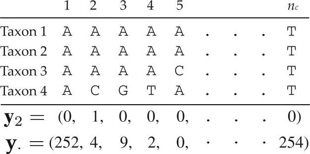
The notation y_i refers to a vector of length n_c that (assuming no missing data or ambiguities) has a single nonzero element (where n_c is the number of possible data patterns). This single nonzero element corresponds to the particular data pattern observed for site i and has value 1. The vector y₂ corresponding to site i = 2 is shown for illustration. The result (y_·) of summing y_i over all i = 1,2,··· ,n_s is also shown (where n_s is the number of sites).

Rather than basing model selection on the marginal likelihood, posterior predictive model selection depends instead on the posterior predictive distribution,

(3)

Here, is the probability of a new data set given the observed data y and model ℳ. The data set may be generated by simulating from model ℳ using a particular set of parameter values θ_ℳ (Fig. 2). The distribution of θ_ℳ, in turn, is provided by the posterior distribution p(θ_ℳ|y,ℳ). A sample from can therefore be obtained by sampling parameters from the posterior distribution (using MCMC), and for each set of parameter values sampled, generating at least one data set by simulation using those parameter values. Several software packages facilitate the simulation of posterior predictive data sets (Rambaut and Grassly 1997; Brown and ElDabaje 2009; Lartillot et al. 2009).

Figure 2.

Generation of posterior predictive data sets under a HKY substitution model for a four-taxon problem. Numbers at the top represent the MCMC iteration at which a posterior sample was drawn, TL=tree length (sum of the five edge length parameters), κ =transition/transversion rate ratio, and π_A, π_C, π_G, π_T =nucleotide equilibrium relative frequencies. For each iteration, the sampled parameter values and tree are used to simulate one data set, the vector of pattern counts of which constitute .

GG APPROACH

The method described by Gelfand and Ghosh (1998), here abbreviated GG, balances the tradeoff between goodness-of-fit and posterior predictive variance. The term “L-measure” (where L stands for “loss”) has been used (Ibrahim et al. 2001; Chen et al. 2004) for this class of Bayesian posterior predictive model selection methods.

We illustrate the GG method using a simple example involving only two taxa, then discuss extending the approach to multiple-taxon sequence alignments. The first column in Table 1 shows the n_c = 4² = 16 patterns possible for two taxa and four nucleotide states, and the remaining three columns represent data sets simulated using the Uniform, JC69, and K80 models. The Uniform model has no free parameters and simply places each new site in one of the 16 bins at random (discrete uniform distribution). The second model is a JC69 model (Jukes and Cantor 1969) with one parameter, the expected number of substitutions per site, or evolutionary distance, ν = 0.5. The third model (K80; Kimura 1980) has two parameters: the evolutionary distance (ν = 0.5 substitutions/site) and the transition/transversion rate ratio (κ = 10). The purpose of this table is to simply show that different models produce different data pattern distributions when asked to simulate data. It is clear from comparing counts for different site patterns that data generated by the Uniform model is strikingly different from data produced by the other two models. The differences between JC69 and K80 are more subtle, but if many data sets were simulated from both of these models, it would be clear that the K80 model consistently produces many more sites representing transition-type substitutions (A ↔ G, C ↔ T) than does the JC69 model.

Table 1.

Examples of pattern counts illustrating the type of information used by the GG method to discriminate among models

Pattern	Uniform	JC69	K80
AA	52	237	196
AC	71	9	2
AG	64	6	23
AT	67	13	2
CA	62	9	3
CC	64	215	255
CG	68	10	1
CT	49	6	24
GA	63	12	18
GC	67	10	1
GG	66	227	207
GT	59	4	2
TA	59	11	3
TC	65	9	29
TG	60	10	3
TT	64	212	231
Lossa	2344.2	0.0	177.7

^aUses the “JC69” column as the reference distribution.

The GG method involves simulating data from a candidate model and comparing the simulated data sets to each other and to the observed data. GG rewards models that do well at producing data sets that are consistently similar to the observed data and punishes models that produce either (i) highly variable data sets (in the sense that replicate simulated data sets bear little resemblance to one another) or (ii) data sets that systematically differ from the observed data. GG does not explicitly penalize a model for having extra parameters: it measures the effect of the model’s parameters with respect to both goodness-of-fit and predictive variance. Models that are too simple tend to fail with respect to goodness-of-fit, and the GG penalizes such models for having poor fit to the observations. Models that are more complex than they need to be tend to produce data that is too variable, and the GG penalizes these models for their gratuitous variability.

Any method using comparisons of simulated data to observed data to assess model performance must solve two problems. First, a model must be parameterized to be used for simulation. For example, if one were to simulate data using the HKY model, what value should be used for the edge lengths (ν), transition/transversion rate ratio (κ), and nucleotide frequencies (π)? We have already seen that choosing ν = 0.5, κ = 1, and π = {0.25,0.25,0.25,0.25} (equivalent to assuming a JC69 model) produces data sets that are noticeably different than when κ = 10 (equivalent to the K80 model). The GG solves this problem by using samples of parameter values from the posterior distribution (obtained during the course of a Bayesian MCMC analysis) to fully specify the model. In this, GG is similar to the posterior predictive P-value approach advocated by Bollback (2002). Second, a means for comparing data sets must be chosen. GG uses loss functions for this purpose.

The Deviance Loss Function

Loss functions are designed such that zero represents a perfect match (i.e., no loss) and larger (strictly positive) values represent increasing amounts of mismatch between the function’s arguments. The GG method is flexible in terms of the loss function used, but in this study, we restrict our attention to the deviance loss function, which is appropriate for comparing discrete categorical data sets such as those encountered in molecular phylogenetics. The deviance loss function used here, L(y,a), compares an observed or simulated data set y with a reference data set a. L(y,a) is, by definition, twice the natural logarithm of the ratio of two probabilities, each of which is a product of categorical probabilities, one for each possible pattern. A categorical probability distribution is appropriate when each observation (y_i) falls into one of n_c bins; the Bernoulli distribution is a special case when the number of bins equals just 2. The quantity p_j is the probability that any given observation falls in bin j (j = 1,··· ,n_c; ∑_j p_j = 1). The joint categorical probability function can be written as

(4)

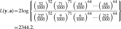
The numerator and denominator of the deviance loss function both take this form and differ only in the choice of values for p_j. A saturated model is used in the numerator: i.e., p_j = y_·j/n_s. In the denominator, the p vector is obtained from the pattern counts composing the reference data set. As an example, let the counts from the “Uniform” column in Table 1 be y and counts from the “JC69” column be a. The deviance loss function is thus

(5)

It is clear that L(y,a) would be zero if the probabilities of site patterns specified by a exactly matched those in the saturated model. Because the saturated model represents the best possible fit to the counts in y, the probability ratio is greater than or equal to 1, guaranteeing that the loss function is greater than or equal to zero. The last row in Table 1 compares loss functions calculated for the example counts, assuming that the “JC69” column represents the reference data set. The largest loss (2344.2) is associated with the data set simulated under the Uniform model, while the “K80” data set is much closer (177.7) to the reference data set “JC69.” In the GG method, loss functions compare either the observed data (y) or a data set () simulated from the posterior predictive distribution to a reference data set a representing a compromise between y and , where k = 1,··· ,n and n is the size of the sample obtained using MCMC from the posterior distribution.

The GG Criterion

The GG criterion for a model ℳis defined as the sum of two terms:

(6)

The first term on the right side measures the expected loss of a posterior predictive data set compared with a reference data set a. The second term measures the loss of the observed data y relative to the same reference data set a, weighted by an arbitrary factor φ that specifies the relative importance of goodness-of-fit compared with predictive variance. A value of φ greater than 1 places more weight on models that fit the observed data well; φ less than 1 emphasizes models with low posterior predictive variance. In this article, φ = 1 is used, a choice supported by theoretical considerations (Ibrahim et al. 2001; Chen et al. 2004). The reference data set a is chosen to minimize the value of GG. That is, the value GG used to compare model ℳto other models is optimized to give model ℳ the best possible chance of being considered the best model. In practice, the reference data set a is a weighted average of the observed data set and all posterior predictive data sets. Thus, unlike the observed data and any of the posterior predictive data sets, a has pattern counts that are not necessarily whole numbers.

It is possible to choose the appropriate a analytically given the form assumed for the loss functions involved. For the deviance loss function, the minimizing a turns out to be

(7)

where y represents the observed data and μ represents the average of the posterior predictive data sets. Each pattern count in μ is a simple average of the counts of the corresponding pattern from all posterior predictive data sets. If φ = 1, then each pattern count in a is a simple average between the count of that pattern in y and μ.

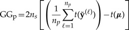
Incorporating the above definition for a into the loss functions reveals that GG can be written as the sum of two components, one (GG_p) directly related to posterior predictive variance and the other (GG_g) directly related to goodness-of-fit:

(8)

(9)

(10)

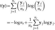
where n_p is the number of posterior predictive data sets generated (n_p ≥ n) and n_s is the total number of sites. The function t(y) is defined as follows:

(11)

The t function is the negative of the nat version of the Shannon entropy measure (Shannon 1948). Thus, it is highest (near its maximum value of zero) when entropy is low (a few patterns dominate) and lowest (near its minimum value of –logn_c, or −logn_s if n_s < n_c) when entropy is high (counts spread evenly over site pattern classes). The value n_c, for DNA sequence data, equals the number of possible patterns, or 4^n_t, but can be much smaller if patterns are combined (see later).

GG_p measures the posterior predictive variance. If the individual posterior predictive data sets are very different from one another, the value of GG_p will be large. If all of the individual posterior predictive data sets were identical, GG_p would equal zero. Lower values of GG_p are desirable in a model because low posterior predictive variance means that the model is consistent in its predictions.

The quantity GG_g measures goodness-of-fit of the model to the observed data. If the posterior predictive data sets are all very similar to the observed data y, then their average μ will also be similar to y and GG_g will be small. GG_g becomes larger as μ and y diverge, which happens only if the posterior predictive out to be data sets generated by the model consistently differ from the observed data.

The goal is thus to find the model with the lowest value of GG. This model best manages the tradeoff between GG_p and GG_g compared with the other models in contention. As with all model choice methods, the values GG_p and GG_g (and thus GG) are relative; models can only be judged better or worse than other models.

The Dimension Problem and a Binned Solution

In the evolutionary distance example presented earlier, there were only 16 possible data patterns, and consequently, a high probability that all 16 pattern counts are nonzero. Increase the number of taxa to match those typical of phylogenetic problems, however, and the number of possible patterns becomes unwieldy, greatly exceeding the number of sites and leading to many patterns with counts equal to zero in y or even in μ. To avoid sparse data vectors, we chose to combine bins to reduce the dimension of the categorical distributions used in the deviance loss function. The GG analyses in this article use the following 15-bin strategy: bins 1–4 represent patterns constant for A, C, G, or T, respectively; bins 5–10 contain patterns composed of two nucleotide states (AC, AG, AT, CG, CT, or GT, respectively); bins 11–14 contain patterns composed of three nucleotide states (ACG, ACT, AGT, or CGT, respectively); and the final bin contains patterns composed of all four nucleotide states. This binning strategy has the advantage of simplicity and wide applicability but is nevertheless arbitrary and other binning strategies may prove to be more effective in capturing the essential features of a data set.

THE CPO APPROACH

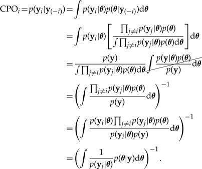
The Conditional Predictive Ordinates (CPO) method represents a posterior predictive approach distinctly different from GG that has proven useful in Bayesian model selection (Geisser 1980; Gelfand et al. 1992; Chen et al. 2000) and which holds promise for exploratory data analysis in Bayesian phylogenetics. The CPO measures the fit of the model to an individual site: specifically, the CPO for a given site i equals p(y_i|y_(−i)): the probability of the data for that site (y_i) conditional on the data (y_(−i)) for all other sites. Its definition also makes CPO a cross-validation method because evaluation of a particular site is based on only data from other sites.

Consider a constant site having (for example) base A for every taxon. If other sites in the sequence yield an estimate of 0.001 for the total tree length, chances are that the focal site is slowly evolving as well. Given the very low substitution rate and reasonably equal base frequencies, the probability of a constant, exclusively-A site is about 0.25. This represents a very high CPO value. Imagine now a contrasting case in which all other sites yield edge length estimates greater than 1.0 for every edge in the tree. In this case, the probability of a constant, exclusively-A site is much lower than 0.25 because all other sites suggest a large amount of substitution, which is inconsistent with a constant site pattern. Interestingly, CPO will generally be low for all sites if substitution rates are high. This is because it is simply inherently difficult to make accurate predictions in the face of a large amount of change. There are very few patterns when substitution is low but very many patterns when substitution is high. Because CPO tends to be inversely proportional to evolutionary rate, CPO can be used to identify fast-evolving regions using a simple model that does not estimate the rate at each site separately.

CPO is attractive because, unlike most cross-validation and posterior-predictive approaches (including GG), no extra simulation is required beyond the MCMC simulation used to sample from the posterior distribution. CPO thus provides, essentially for free, a measure of both overall and site-specific model fit using samples from the same MCMC analysis used to estimate model parameters and the tree topology. Examination of a plot of CPO values can identify regions of sequences that, for one reason or another (incorrect alignment, differing nucleotide composition, etc.), exhibit poor model fit compared with the majority of sites.

CPO and Log Pseudomarginal Likelihood

Letting y_(−i) denote data from all sites except i, the CPO for the ith site (CPO_i) emerges as the posterior harmonic mean of the ith site likelihood:

(12)

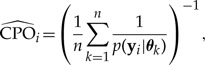
(The Appendix discusses the relationship of CPO to the harmonic mean method for estimating marginal likelihood.) Although counterintuitive, equation (12) shows that it is possible to perform cross validation (computing the probability of the data from one site given data from all other sites) without the necessity of performing n_s separate analyses. Equation (12) suggests the following MCMC approximation (Chen et al. 2000, eq. 10.1.9, p. 310):

(13)

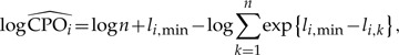
where θ_k is the kth sampled parameter vector from an MCMC analysis targeting the posterior distribution (k = 1,··· ,n). The quantity p(y_i|θ_k) is generally only available on the log scale, so the following provides a more useful computing formula:

(14)

where l_i,k = logp(y_i|θ_k) is the site likelihood for the ith site computed using the kth sampled parameter vector, and l_i,min = min{l_i,k : k = 1,··· ,n}.

The log pseudomarginal likelihood (LPML) is obtained by summing the n_s individual site values:

(15)

EXAMPLES

Data Sets

The following two data sets were used in the examples that follow. The alignments used are available in the supplementary materials (Dryad data repository, doi:10.5061/dryad.6b7c1) associated with this article.

Algae Protein-Coding Plastid Data Set.—These data are from four protein-coding plastid genes (psaA, psaB, psbC, and rbcL) in chlorophyceaen green algae (Tippery et al. 2012, treebase.orgstudy number 11663). Seven taxa with more than 20% missing data and 537 sites with missing data in more than 5% of taxa were removed, leaving 28 taxa and 5487 sites.

Angiosperm Ribosomal Protein Data Set.—These data are from the rps11 ribosomal protein gene in five angiosperms (Bergthorsson et al. 2003; nature.com, supplementary information). The original data set comprised 47 taxa and was determined by Bergthorsson et al. (2003) to be chimeric in the dicot Sanguinaria canadensis (bloodroot): the 237 nucleotides at the 3^′ end of the gene (456 sites total) apparently resulted from a horizontal transfer from a monocot mitochondrion. When reduced to the five taxa reanalyzed here, 54 sites had only gaps and were excluded from the analysis, yielding 180 sites in the 5^′ end and 222 sites in the 3^′ end (402 sites total).

Example 1: GG and Edge Length Priors

Ideally, Bayesian model selection methods should be sensitive to cases in which informative priors negatively affect model performance. We conducted a series of analyses differing only in the assumed edge length prior distributions. All edge length priors were exponential distributions, a common choice in Bayesian phylogenetic studies. The exponential distribution is a special case of the gamma distribution in which the standard deviation equals the mean. Exponential distributions with smaller means are more informative when used as prior distributions due to their smaller variance. Furthermore, because the prior is applied to every edge length parameter, and there are often many such parameters (2n_t − 3 for unrooted trees), the choice of edge length prior distribution often has a much greater impact than prior choices made for most other model parameters. In fact, what appears to be a very reasonable edge length prior may induce a very informative (often unreasonably so) prior on the tree length (Brown et al. 2010; Rannala et al. 2011). The sum of n_e independent edge lengths, each of which has an exponential (λ) distribution (mean 1/λ, variance 1/λ²), is a tree length with a gamma (n_e, λ⁻¹) distribution (mean n_e/λ, variance n_e/λ²), also known as an Erlang distribution. Such induced tree length priors have been known to strongly affect the scaling of edge lengths in the posterior distribution. For example, Marshall (2010) reports an analysis of mitochondrial protein-coding data from cicadas in which the tree length was estimated to be 7.7 despite evidence that 1.5 is closer to the true value. For this 51-taxon study, the exponential edge length prior with mean 0.1 induced a gamma tree length prior having mean 9.9 and standard deviation 0.99, suggesting that the estimated tree length of 7.7 resulted from a tug-of-war between the likelihood, which was arguing for something close to 1.5, and the prior, which was arguing for 9.9. Brown et al. (2010) provide examples in which the posterior distribution of tree length is clearly being determined largely by the edge length prior. For the “clams” data and “large” mean edge length prior, the interval containing the middle 95% of the induced Erlang prior on tree length was (157.4, 210.4), nearly identical to the 95% credible interval, (156.5, 208.2). The maximum likelihood tree length, by comparison, was only 1.96!

The data used for the following example were from the psaB gene in the algae protein-coding plastid data set. Figure 3 shows results from eight independent analyses, each using a different prior model for edge lengths. The General Time Reversible substitution model with discrete gamma among-site rate heterogeneity (GTR+G) and partitioning scheme (partitioned by codon position) were identical across models. Flat Dirichlet priors were used for state frequencies and GTR exchangeabilities, an exponential (1) prior was used for the four-category discrete gamma shape parameter, and a flat relative rate prior (Fan et al. 2011) was used for the partition subset relative rates. Tree diagrams below the plot show the final tree sampled from each analysis. It is clear that as exponential edge length prior means become not only smaller but also more informative, the number of distinct data patterns in posterior predictive data sets drops and goodness-of-fit decreases (i.e., G rises). The P component of GG did not have any appreciable effect, suggesting that none of the models produced posterior predictive data sets that strongly differed from the mean. Figure 3 makes it clear that for these data it is better to err on the side of larger means for exponential edge length priors (but note that studies such as Brown et al. (2010) suggest this result may not generalize). GG was nearly constant for prior means ranging from 10 down to 0.01, but prior means smaller than 0.01 had a clearly negative impact on G, producing many more constant patterns and many fewer variable patterns than were present in the observed data. Interestingly, the best choice for prior mean was 0.01, which falls at a point where the tree length shortening effect of the edge length prior is becoming clearly evident. For these data, the maximum likelihood estimate of tree length was 8.2 based on a GARLI 2.0 (Zwickl 2006) analysis using the same model and partitioning scheme. This tree length is the sum of 67 edge lengths (unrooted tree of 35 taxa), yielding an average edge length of 0.12, which is an order of magnitude larger than the best prior mean edge length (0.01).

Figure 3.

Comparison of prior models using the GG criterion for the gene psaB in the algae example data set. Solid line with squares: the mean number of distinct data patterns in posterior predictive data sets. Solid line with open circles: the overall GG measure (smallest is best). Dashed line with downward-pointing triangles: the goodness-of-fit component (GG_g) of the GG criterion. Dotted line with upward-pointing triangle: the variance component GG_p of the GG criterion. Trees shown below the plot are the last tree sampled for each of the eight analyses. The prior mean used for each analysis is 10^x, where x is the abscissa, except for the point labeled “hyper” in which the exponential prior mean was a hyperparameter in a hierarchical model.

One model (labeled “hyper”) used a hyperparameter as the mean of the separate exponential edge length priors applied to internal and external edge lengths. The hyperprior for this model was inverse gamma prior (mean 1, variance 10), as suggested by Suchard et al. (2001). Using a hierarchical model allows the prior mean to be estimated from the data, relieving the investigator of the burden of having to choose the edge length prior mean. The estimated edge length hyperparameters were 0.12 (internal) and 0.18 (external), which are both close to the maximum likelihood average edge length (0.12). The empirical Bayesian edge length prior suggested by Brown et al. (2010) would have mean 0.17, slightly larger than the maximum likelihood average edge length (0.12) and close to the estimated external edge length hyperparameter in the hierarchical model (0.18).

Why is the GG choice an order of magnitude smaller than both the maximum likelihood estimate and the posterior mean hyperparameter values? It is important to point out that GG judges models on their ability to generate data sets that consistently and accurately mimic the observed data, and a model that does well at this task can win out regardless of how well it fits the observed data (as measured by the likelihood). Placing weak constraints on edge lengths, keeping edge lengths slightly shorter than their maximum likelihood estimates, tends to slightly improve the predictive ability of the model in this case. The improvement in GG of the best model over the hierarchical model is minor, however, and this example illustrates the fact that the hierarchical approach does quite well at automatically choosing appropriate values for prior means.

Example 2: CPO Analysis of Green Algal Protein-Coding Data

Our second example is designed to illustrate how CPO can be used to learn about evolutionary rates using a simple model of evolution (GTR+G). The data comprise portions of four protein-coding genes (psaA, psaB, psbC, and rbcL) from the algae protein-coding plastid data set. Figure 4a plots CPO_i for each site i when data are partitioned by gene. The tree topology and edge lengths are linked across partition subsets, but otherwise the parameters (nucleotide relative frequencies, GTR exchangeability parameters, and the discrete-gamma shape parameter used to model among-site relative rates) of a GTR+G model were estimated separately for each subset. Each subset was allowed its own edge length scaler, accommodating differences in relative rate of substitution across subsets. Flat Dirichlet priors were used for state frequencies and GTR relative rates, an exponential(1) prior was used for the four-category discrete gamma shape parameter, a single exponential prior was used for every edge length, with mean a hyperparameter for which the hyperprior was an inverse gamma prior (mean 1, variance 10) distribution, and a flat relative rate prior was used for subset relative rates. Dotted lines in Figure 4a denote gene boundaries.

Figure 4.

Plots of site-specific log(CPO) values for analyses of all four genes in the algae data set. a) Partitioned by gene (dotted vertical lines show gene boundaries). b) Partitioned by gene, but sorted by codon position, with 1st (left), 2nd position (center), and 3rd position (right) (dotted vertical lines show codon position boundaries). c) Partitioned by codon (dotted vertical lines show codon position boundaries).

Plotting the same log-CPO values by codon position (Fig. 4b) clearly shows a relationship between CPO and the rate of evolution. Third codon positions have the highest average relative rate and the lowest average CPO values, while second positions have the lowest rates and highest CPO values. Importantly, even if the model was able to perfectly estimate edge lengths, low CPO values would nevertheless be expected if the (true) tree length was large such that many substitutions have occurred per site. High substitution rates yield complex data patterns that are difficult to predict even if the model fits perfectly. On the other hand, low rates yield simple patterns (e.g., constant patterns) that are much easier to predict. Although CPO values improve with models that accommodate among-site rate heterogeneity, this basic relationship between rate and CPO remains.

Also important to keep in mind is the fact that completely missing data can be perfectly predicted because any pattern suggested constitutes a successful prediction. Hence, sites with a high proportion of missing data yield high CPO values. In these data, sites with greater than 5% missing data were removed. If these sites had been included, a clear increase in CPO near gene boundaries would be evident due to the increased amount of missing data near the start and end of each gene.

The pattern of CPO values suggests that partitioning by codon position rather than by gene would improve the model. Figure 4c plots site-specific log-CPO values for the case of a partition with three subsets corresponding to first, second, and third codon position. Again, tree topology and edge lengths were linked across subsets, and otherwise, each subset got its own GTR+G model. Although Figure 4c looks remarkably similar to Figure 4b, the LPML for the codon partitioning model (−54,868) is much higher than the LPML for the gene partitioning model (−58,414), indicating that allowing codon positions to have their own relative rates substantially improves the model’s predictive ability.

Example 3: CPO Analysis of Angiosperm rps11

Bergthorsson et al. (2003) discovered that the ribosomal protein gene rps11 is chimeric in the angiosperm Sanguinaria (“bloodroot”). The 5′ end of the gene (219 nucleotides) supports a tree topology consistent with vertical transmission (i.e., Sanguinaria falls within the family of angiosperms, Papaveraceae, in which it is classified). The 3′ end of the gene (237 nucleotides) supports a tree topology consistent with horizontal transfer from a mitochondrion within the monocots. To illustrate the value of CPO in exploratory data analyses, we conducted two separate Bayesian MCMC analyses of a five-taxon version of the rps11 data set. In both analyses, the tree topology was fixed and the model used was GTR+G, with flat Dirichlet priors on GTR exchangeabilities and nucleotide frequencies, an exponential(1) prior on the shape parameter governing the four-category discrete gamma distribution of relative among-site rates, and an inverse gamma prior (mean 1, variance 10) governing the mean of an exponential prior applied to all edge lengths. Each MCMC analysis involved 101,000 cycles (one cycle involves an update of all model parameters), with the first 1000 discarded as burn-in and the remaining run sampled every 100 cycles to yield 1000 total samples from the posterior distribution. CPO values were computed using equation (14).

In the first of the two analyses the 5^′ tree topology (in which Sanguinaria groups with confamilial genera Bocconia and Eschscholzia) was fixed. The site-specific CPO values estimated from this analysis were recorded as CPO5. In the second analysis, the 3^′ tree topology (in which Sanguinaria groups with the monocot genera Oryza and Disporum) was fixed. The site-specific CPO values estimated from this analysis were recorded as CPO3. We expected that CPO3 would be greater than CPO5 in the 3^′ end of the gene in which history coincides with the 3^′ tree. Likewise, we expected that CPO5 would exceed CPO3 in the 5^′ end of the gene, where history coincides with the 5^′ tree. Figure 5 plots the difference CPO3-CPO5 (vertical axis) as a function of site index (horizontal axis). The vertical dotted line indicates the change point where history switches from the 5^′ tree topology (shown on left) to the 3^′ tree topology (shown on right). As expected, most of the CPO differences are negative in the 5^′ end of the gene (to the left of the dotted line), and most differences are positive in the 3^′ end of the gene (to the right of the dotted line). All exceptions to this rule are associated with autapomorphic patterns in which all taxa are identical in state except for one.

Figure 5.

Plot of the log of the CPO ratio, equal to log(CPO3) −log(CPO5), where CPO5 is site-specific CPO estimated using the 5′ tree (on left), and CPO3 is site-specific CPO estimated using the 3′ tree (on right). Vertical dotted line separates 5′ end (left) from 3′ end (right) of the ribosomal protein gene rps11.

Example 4: Partition Model Selection

The last example compares GG and CPO with a marginal likelihood estimation method (SS; Fan et al. 2011) in assessing the relative merits of four different partitioning schemes for the algal protein coding data. The four partitioning schemes compared were: NONE (no partitioning); GENE (four subsets, one for each of the four genes: psaA, psaB, psbC, and rbcL); CODON (three subsets, one for each codon position); and BOTH (12 subsets, one for each codon position of each gene). In each case, each subset was provided its own GTR+I+G model, with flat Dirichlet priors applied to state frequencies and GTR exchangeabilities, an exponential(1) prior applied to the shape parameter of the four-category discrete gamma rate heterogeneity submodel, and an inverse gamma (mean 1, variance 10) hyperparameter governing the mean of the exponential prior applied to each edge length. A flat relative rate prior was applied to the subset relative rates. Figure 6 and Table 2 summarize the results. Note that better models are associated with higher SS and CPO scores but lower GG. All three model selection methods favored CODON/BOTH over NONE/GENE, suggesting that rate heterogeneity among codon positions is much greater than rate heterogeneity among genes. According to the two posterior predictive methods, GG and CPO, GENE was slightly better than NONE, and BOTH was slightly better than CODON. In contrast to the two posterior predictive methods, marginal likelihoods estimated using the SS method preferred CODON to BOTH.

Figure 6.

Comparison of partition models for green algal protein-coding data. NONE is unpartitioned, GENE is partitioned by gene (four subsets), CODON is partitioned by codon position (three subsets), and BOTH is partitioned by both gene and codon position (12 subsets). Squares indicate GG, circles indicate SS, and triangles indicate LPML. Solid lines use scale on left; dotted line uses scale on right.

Table 2.

Comparison of partition models using SS, LPML, GG, variance penalty component of GG (GG_p), and goodness-of-fit component of GG (GG_g)

Model	Subsets	Parametersa	SS	LPML	GG	GGp	GGg
NONE	1	63	−58,561.4	−59,200.2	1325.0	46.5	1278.5
GENE	4	96	−58,499.9	−59,097.9	1084.2	14.6	1069.6
CODON	3	85	−54,980.5	−56,367.3	357.4	15.9	341.5
BOTH	12	184	−55,019.0	−56,339.2	301.9	16.2	285.7

Note: Bold denotes best value across models.

^aThe number of free parameters equals 53+10n_subsets + (n_subsets − 1), where 53 is the number of edge lengths, n_subsets is the number of subsets, and 10 is the number of free parameters in the GTR+I+G model.

DISCUSSION

Gelfand–Ghosh

Bollback (2002, 2005) was the first to introduce posterior predictive approaches into Bayesian phylogenetic model selection. Bollback’s posterior predictive P-value method involved computing the following statistic for both the observed data set y and for each posterior predictive data set :

(16)

If T(y) lies in the tail of the distribution formed by the values, then the model is considered an inadequate description of the observed data. There are two potential criticisms of this approach. First, Bollback’s method does not penalize a model for excessive posterior predictive variance. In fact, P-value approaches reward large posterior predictive variance: given a broad enough distribution of nearly any observed data set can avoid being in the tail. Second, the categorical test statistic depends only on the counts associated with site patterns and not the patterns themselves. Thus, two data sets that are extremely different can potentially have identical numerical values for this statistic. Foster (2004) found that a different test statistic—the χ² test statistic described by Huelsenbeck et al. (2001)—worked much better than the categorical test statistic, but the χ² statistic is designed specifically for detecting changes in nucleotide composition across a tree. Although there is no evidence that either pitfall described above occurs at a frequency high enough to cause concern, the GG method addresses both criticisms, rewarding models for high goodness-of-fit, punishing them for being vague in their predictions, and using the data patterns themselves and not just the pattern counts in the criterion.

The deviance loss function used with GG, unlike Bollback’s categorical test statistic, is attentive to pattern identities as well as pattern counts; however, as implemented here, the GG method is not without its own criticisms. Although the binning strategy we use with GG is designed to capture salient nucleotide composition and variability in data sets, the choice to reduce all data sets to just 15 bins is arbitrary and may result in the loss of information important in model selection. We note that L-measures in general, including the class of methods introduced by Gelfand and Ghosh (1998), are very general; our GG is a special case tailored specifically to nucleotide sequence data sets, and the limitations we discuss here do not apply to all applications of L-measures. In future work, we plan to investigate additional binning strategies as well as alternative loss functions. Another potential criticism involves missing data. Our GG implementation does not address missing data explicitly. For example, a constant pattern consisting solely of the nucleotide A (adenosine monophosphate) for all taxa except for one, which is scored as missing data, would be added to bin 1 in our scheme (patterns constant for A). Arguably, such patterns should be fractionally distributed among all bins consistent with possible resolutions of the missing data. More elegant solutions can be imagined that involve data augmentation, that is, filling in values for all missing data using the model under consideration, but the details are yet to be elucidated. Despite these potential pitfalls, the GG method behaved reasonably in the partitioning example, corroborating the major results of the SS and CPO analyses.

Conditional Predictive Ordinates

The CPO provides a measure of how well the data pattern from each site in a sequence alignment is predicted by the model. Summing site-log-CPO values provides a model log-CPO value, the LPML, that can be used to compare models with respect to their predictive ability. Even though both use the posterior predictive distribution, CPO is qualitatively different than GG, and both methods offer perspectives that the other cannot provide. CPO evaluates the posterior predictive probability density but does not simulate from it, and thus lacks GG’s ability to measure posterior predictive variance. On the other hand, GG lacks the cross validation that CPO provides (each site is evaluated using a model parameterized from all other sites). Both methods require minimal computational effort beyond that required to obtain a sample from the posterior distribution.

Besides providing its own unique perspective on model selection, there are other possible uses for CPO. Very low CPO values may be useful in identifying regions of alignments where positional homology is suspect. A region of low CPO in a sequence suggests that those particular sites may have evolved under a different model (substitution model or tree model) than the majority of sites (see rps11 example and Fig. 5). The correlation of CPO with rate of evolution allows CPO to be used as a proxy for relative substitution rates. Rather than performing an analysis under a parameter-rich model in which every site is allowed to have its own substitution rate, an analysis using a simple model with a single substitution rate can produce site-specific CPO values that are highly correlated with substitution rates of individual sites. In this way, it is similar to the TIGER method (Cummins and McInerney 2011), which uses a measure of pairwise character compatibility as a proxy for rate, assuming that high-rate sites will also be those that are incompatible with many other sites. Lack of dependence on both substitution model and tree are strengths of the TIGER approach; however, CPO might offer some advantages over TIGER in terms of accuracy because it uses a substitution model. For example, plastid-encoded third position sites, such as those in the algae data set used in this article, exhibit a strong AT bias (estimated π_A + π_T = 0.88), information that is relevant to assessment of substitution rates but which TIGER does not use. Likewise, CPO uses information about the tree and edge lengths, while also accounting for uncertainty in both. TIGER and CPO provide complimentary approaches: CPO provides a more accurate proxy for substitution rates given that its dependence on a model does not lead to systematic error, while TIGER provides a less accurate proxy but is less subject to model misspecification.

Posterior Predictive versus Marginal Likelihood Approaches

Bayesian model selection in phylogenetics is dominated by marginal likelihood methods (including Bayes factors, which are ratios of marginal likelihoods). Phylogenetics is blessed with a diversity of marginal likelihood/Bayes factor estimation methods from which to choose, including Savage-Dickey ratio (Suchard et al. 2001), harmonic mean (Newton and Raftery 1994), thermodynamic integration (Lartillot and Phillippe 2006; Lepage et al. 2007), SS (Fan et al. 2011; Xie et al. 2011), inflated density ratio (Arima and Tardella 2012), and reversible-jump MCMC (Huelsenbeck et al. 2004). Why is it important to add posterior predictive methods to this list? One key difference between marginal likelihood and posterior predictive approaches lies in the fact that the marginal likelihood measures the fit of the model to the observed data. How well would that model fit a different data set? For example, suppose a different set of genes was sampled, or different populations of the species involved were sampled for the same set of genes? The marginal likelihood is not designed to predict how well a model would perform on data sets other than the one observed, yet it is clear that such performance might be important to a researcher.

Posterior predictive methods play a similar role in Bayesian statistics that parametric bootstrapping plays in maximum likelihood analyses: They take into account the extra uncertainty that comes with no longer assuming that the only data set is the observed data set. As such, posterior predictive model selection methods complement the opinion provided by methods based on marginal likelihood. An implicit assumption of the marginal likelihood approach to model selection is that a model fitting the observed data well would also generate data sets by simulation that are similar to the observed data. Posterior predictive approaches such as GG address this issue explicitly.

A major goal of modeling is prediction. Hurricane forecasters are concerned with the literal meaning of prediction, whereas “interpolation accuracy” might be a better term to use in the phylogenetics context. In a regression context, a simple linear model might perform better at predicting the dependent variable for as-yes-unmeasured values of the independent variable than a complex polynomial model whose regression line goes through every observed point at the cost of looping absurdly between the observations. We do not need the model to help us with the observed data; instead, models are needed to interpolate between the observations. It is for this reason that the perspective offered by posterior predictive methods is valuable.

APPENDIX

The Delta method can be used to compare the critical second moment terms of the harmonic mean estimator of the marginal likelihood with the corresponding term in the harmonic mean estimator of the CPO. We demonstrate that although the two methods both involve a harmonic mean of site likelihoods, their numerical properties and associated statistical behavior are expected to be very different. In particular, the CPO estimator is not expected to share the instability and infinite variance that characterizes the harmonic mean marginal likelihood estimator. Later, we explain the fundamental difference between the two methods and show why the CPO estimator is expected to be well behaved but do not attempt a general proof.

Harmonic Mean Estimator of Marginal Likelihood

The harmonic mean estimator of the marginal likelihood is

(A1)

based on n draws θ₁,θ₂,...,θ_n from the posterior distribution p(θ|y). The estimator is consistent but may have infinite variance across simulation, even in simple models. Defining

(A2)

(A3)

the Delta method yields

(A4)

Focusing on the variance term,

(A5)

Thus,

(A6)

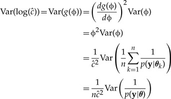
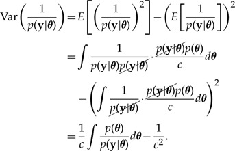
The key term in the variance in equation (A6) corresponds to the second moment of Var (p(y|θ)⁻¹),

(A7)

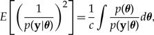
which consists of a denominator, p(y|θ), that is much more concentrated than the numerator, p(θ), due to its large number of terms (one site likelihood term for every site). In particular, the tail regions of the denominator can be very tiny compared with their counterparts in the numerator, making the variance on the log scale unstable, leading to potentially infinite variance when translated to the standard scale.

Comparison with CPO Estimator

The CPO, CPO_i, for the ith site can be estimated from n independent draws θ₁,θ₂,...,θ_n from the posterior distribution p(θ|y) as follows:

(A8)

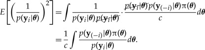
Equation (A8) is nearly identical to equation (A1), but repeating the analysis above reveals a key difference in the second moment in the case of CPO:

(A9)

Note that the second moment for CPO places all but one site likelihood term in the numerator. In this case, the numerator normally is more concentrated and exhibits very long, low tails, whereas the denominator is more diffuse owing to the fact that it represents a single site-likelihood term. This construction is not likely to produce extremely large values, leading to a more stable variance on the log scale and finite variance on the standard scale.

SOFTWARE AVAILABILITY

The free and open-source software Phycas (http://www.phycas.org/) implements both the GG and CPO methods for standard nucleotide models (GTR+I+G and submodels) and partitioned or unpartitioned data sets.

SUPPLEMENTARY MATERIAL

Data files and/or other supplementary information related to this paper have been deposited at Dryad under doi:10.5061/dryad.6b7c1.

FUNDING

This work was supported by the National Science Foundation [DEB-1036448 to P.O.L.] (GrAToL); and the National Institutes of Health [GM 70335 and CA 74015 to M.H.C.].

REFERENCES

- Akaike H. A new look at statistical model identification. IEEE Trans. Automat. Contr. 1974;19:716–723. [Google Scholar]
- Arima S., Tardella L. Improved harmonic mean estimator for phylogenetic model evidence. J. Comput. Biol. 2012;19:418–438. doi: 10.1089/cmb.2010.0139. [DOI] [PubMed] [Google Scholar]
- Baele G., Lemey P., Bedford T., Rambaut A., Suchard M.A., Alekseyenko A.V. Improving the accuracy of demographic and molecular clock model comparison while accommodating phylogenetic uncertainty. Mol. Biol. Evol. 2012;29:2157–2167. doi: 10.1093/molbev/mss084. [DOI] [PMC free article] [PubMed] [Google Scholar]
- Bergthorsson U., Adams K.L., Thomason B., Palmer J.D. Widespread horizontal transfer of mitochondrial genes in flowering plants. Nature. 2003;424:197–201. doi: 10.1038/nature01743. [DOI] [PubMed] [Google Scholar]
- Bollback J. Bayesian model adequacy and choice in phylogenetics. Mol. Biol. Evol. 2002;19:1171–1180. doi: 10.1093/oxfordjournals.molbev.a004175. [DOI] [PubMed] [Google Scholar]
- Bollback J.P. Posterior mapping and predictive distributions. In: Nielsen R., editor. Statistical methods in molecular evolution. New York: Springer Verlag; 2005. pp. 439–462. [Google Scholar]
- Brown J.M., ElDabaje R. PuMA: Bayesian analysis of partitioned (and unpartitioned) model adequacy. Bioinformatics. 2009;25:537–538. doi: 10.1093/bioinformatics/btn651. [DOI] [PubMed] [Google Scholar]
- Brown J.M., Hedtke S.M., Lemmon A.R., Lemmon E.M. When trees grow too long: investigating the causes of highly inaccurate Bayesian branch-length estimates. Syst. Biol. 2010;59:145–161. doi: 10.1093/sysbio/syp081. [DOI] [PubMed] [Google Scholar]
- Chen M.-H., Dey D., Ibrahim J. Bayesian criterion based model assessment for categorical data. Biometrika. 2004;91:45–63. [Google Scholar]
- Chen M.-H., Shao Q.-M., Ibrahim J.G., editors. New York: Springer; 2000. Monte Carlo methods in Bayesian computation. [Google Scholar]
- Cummins C.A., McInerney J.O. A method for inferring the rate of evolution of homologous characters that can potentially improve phylogenetic inference, resolve deep divergence and correct systematic biases. Syst. Biol. 2011;60:833–844. doi: 10.1093/sysbio/syr064. [DOI] [PubMed] [Google Scholar]
- Fan Y., Wu R., Chen M.-H., Kuo L., Lewis P.O. Choosing among partition models in Bayesian phylogenetics. Mol. Biol. Evol. 2011;28:523–532. doi: 10.1093/molbev/msq224. [DOI] [PMC free article] [PubMed] [Google Scholar]
- Foster P.G. Modeling compositional heterogeneity. Syst. Biol. 2004;53:485–495. doi: 10.1080/10635150490445779. [DOI] [PubMed] [Google Scholar]
- Friel N., Pettitt A.N. Marginal likelihood estimation via power posteriors. J. Roy. Stat. Soc. B. 2008;70:589–607. [Google Scholar]
- Geisser S. In discussion of G. E. P. Box paper entitled: Sampling and Bayes' inference in scientific modelling and robustness. J. Roy. Stat. Soc. A. 1980;143:416–417. [Google Scholar]
- Gelfand A.E., Dey D.K., Chang H. 1992. Model determination using predictive distributions with implementation via sampling-based methods (with discussion) Department of Statistics, Stanford University, Tech. Rep., Stanford, California, 462. [Google Scholar]
- Gelfand A.E., Ghosh S. Model choice: a minimum posterior predictive loss approach. Biometrika. 1998;85:1–11. [Google Scholar]
- Guindon S., Dufayard J.F., Lefort V., Anisimova M., Hordijk W., Gascuel O. New algorithms and methods to estimate maximum-likelihood phylogenies: assessing the performance of PhyML 3.0. Syst. Biol. 2010;59:307–321. doi: 10.1093/sysbio/syq010. [DOI] [PubMed] [Google Scholar]
- Huelsenbeck J.P., Larget B., Alfaro M.E. Bayesian phylogenetic model selection using reversible jump Markov chain Monte Carlo. Mol. Biol. Evol. 2004;21:1123–1133. doi: 10.1093/molbev/msh123. [DOI] [PubMed] [Google Scholar]
- Huelsenbeck J.P., Ronquist F., Nielsen R., Bollback J.P. Bayesian inference of phylogeny and its impact on evolutionary biology. Science. 2001;294:2310–2314. doi: 10.1126/science.1065889. [DOI] [PubMed] [Google Scholar]
- Ibrahim J., Chen M., Sinha D. Criterion-based methods for Bayesian model assessment. Stat. Sinica. 2001;11:419–443. [Google Scholar]
- Jukes T.H., Cantor C.R. Evolution of protein molecules. In: Munro H.N., editor. Mammalian protein metabolism. New York: Academic Press; 1969. pp. 21–132. [Google Scholar]
- Kimura M. A simple method for estimating evolutionary rates of base substitutions through comparative studies of nucleotide sequences. J. Mol. Evol. 1980;16:111–120. doi: 10.1007/BF01731581. [DOI] [PubMed] [Google Scholar]
- Lartillot N., Lepage T., Blanquart S. PhyloBayes 3: a Bayesian software package for phylogenetic reconstruction and molecular dating. Bioinformatics. 2009;25:2286–2288. doi: 10.1093/bioinformatics/btp368. [DOI] [PubMed] [Google Scholar]
- Lartillot N., Phillippe H. Computing Bayes factors using thermodynamic integration. Syst. Biol. 2006;55:195–207. doi: 10.1080/10635150500433722. [DOI] [PubMed] [Google Scholar]
- Lepage T., Bryant D., Philippe H., Lartillot N. A general comparison of relaxed molecular clock models. Mol. Biol. Evol. 2007;24:2669–2680. doi: 10.1093/molbev/msm193. [DOI] [PubMed] [Google Scholar]
- Marshall D.C. Cryptic failure of partitioned Bayesian phylogenetic analyses: lost in the land of long trees. Syst. Biol. 2010;59:108–117. doi: 10.1093/sysbio/syp080. [DOI] [PubMed] [Google Scholar]
- Newton M.A., Raftery A.E. Approximate Bayesian inference with the weighted likelihood bootstrap (with discussion) J. Roy. Stat. Soc. B. 1994;56:3–48. [Google Scholar]
- Nylander J.A.A. MrModeltest v2.3. Uppsala, Sweden: Evolutionary Biology Centre, Uppsala University; 2008. Distributed by the author. [Google Scholar]
- Posada D. jModelTest: phylogenetic model averaging. Mol. Biol. Evol. 2008;25:1253–1256. doi: 10.1093/molbev/msn083. [DOI] [PubMed] [Google Scholar]
- Posada D., Crandall K.A.. MODELTEST: testing the model of DNA substitution. Bioinformatics. 1998;14:817–818. doi: 10.1093/bioinformatics/14.9.817. [DOI] [PubMed] [Google Scholar]
- Rambaut A., Grassly N.C. Seq-Gen: an application for the Monte Carlo simulation of DNA sequence evolution along phylogenetic trees. Comput. Appl. Biosci. 1997;13:235–238. doi: 10.1093/bioinformatics/13.3.235. [DOI] [PubMed] [Google Scholar]
- Rannala B., Zhu T., Yang Z. Tail paradox, partial identifiability, and influential priors in Bayesian branch length inference. Mol. Biol. Evol. 2011;29:325–335. doi: 10.1093/molbev/msr210. [DOI] [PubMed] [Google Scholar]
- Ripplinger J., Sullivan J. Assessment of substitution model adequacy using frequentist and Bayesian methods. Mol. Biol. Evol. 2010;27:2790–2803. doi: 10.1093/molbev/msq168. [DOI] [PMC free article] [PubMed] [Google Scholar]
- Ronquist F., Teslenko M., Van Der Mark P., Ayres D.L., Darling A., Höhna S., Larget B., Liu L., Suchard M.A., Huelsenbeck J.P. MrBayes 3.2: efficient Bayesian phylogenetic inference and model choice across a large model space. Syst. Biol. 2012;61:539–542. doi: 10.1093/sysbio/sys029. [DOI] [PMC free article] [PubMed] [Google Scholar]
- Schwarz G.E. Estimating the dimension of a model. Ann. Statist. 1978;6:461–464. [Google Scholar]
- Shannon C.E. A mathematical theory of communication. AT&T Tech. J. 1948;27:379–423. 623–656. [Google Scholar]
- Suchard M., Weiss R., Sinsheimer J. Bayesian selection of continuous-time Markov chain evolutionary models. Mol. Biol. Evol. 2001;18:1001–1013. doi: 10.1093/oxfordjournals.molbev.a003872. [DOI] [PubMed] [Google Scholar]
- Sullivan J., Joyce P. Model selection in phylogenetics. Ann. Rev. Ecol. Evol. S. 2005;36:445–466. [Google Scholar]
- Swofford D.L. Sunderland (MA): Sinauer Associates; 2002. PAUP*: phylogenetic analysis using parsimony (*and other methods) [Google Scholar]
- Tippery N.P., Fučíková K., Lewis P.O., Lewis L.A. Probing the monophyly of the directly opposite flagellar apparatus group in Chlorophyceae using data from five genes. J. Phycol. 2012;48:1482–1493. doi: 10.1111/jpy.12003. [DOI] [PubMed] [Google Scholar]
- Wilks S.S. The large-sample distribution of the likelihood ratio for testing composite hypotheses. Ann. Statist. 1938;9:60–62. [Google Scholar]
- Xie W., Lewis P.O., Fan Y., Kuo L., Chen M.-H. Improving marginal likelihood estimation for Bayesian phylogenetic model selection. Syst. Biol. 2011;60:150–160. doi: 10.1093/sysbio/syq085. [DOI] [PMC free article] [PubMed] [Google Scholar]
- Zwickl D.J. University of Texas at Austin; 2006. Genetic algorithm approaches for the phylogenetic analysis of large biological sequence datasets under the maximum likelihood criterion [Ph.D. thesis] [Google Scholar]