Exploring the Structure of the 100 Amino-Acid Residue Long N-Terminus of the Plant Antenna Protein CP29

Abstract

The structure of the unusually long (∼100 amino-acid residues) N-terminal domain of the light-harvesting protein CP29 of plants is not defined in the crystal structure of this membrane protein. We studied the N-terminus using two electron paramagnetic resonance (EPR) approaches: the rotational diffusion of spin labels at 55 residues with continuous-wave EPR, and three sets of distances with a pulsed EPR method. The N-terminus is relatively structured. Five regions that differ considerably in their dynamics are identified. Two regions have low rotational diffusion, one of which shows α-helical character suggesting contact with the protein surface. This immobile part is flanked by two highly dynamic, unstructured regions (loops) that cover residues 10–22 and 82–91. These loops may be important for the interaction with other light-harvesting proteins. The region around residue 4 also has low rotational diffusion, presumably because it attaches noncovalently to the protein. This section is close to a phosphorylation site (Thr-6) in related proteins, such as those encoded by the Lhcb4.2 gene. Phosphorylation might influence the interaction with other antenna complexes, thereby regulating the supramolecular organization in the thylakoid membrane.

Introduction

In higher plants, photosynthesis is performed by two multiprotein complexes, photosystem (PS) I and II, which are composed of a core complex and an outer antenna part (1,2). In PSII, the outer antenna system is built from a large number of complexes, the most relevant of which for this work are LHCII, the major antenna subunit, and three minor complexes, CP24, CP26, and CP29 (1,3). Among the minor complexes, CP29 is the largest one and is believed to collect, conduct, and possibly quench electronic excitation energy in photosynthesis (1,3–13). Moreover, CP29 is essential for the proper assembly of PSII and its absence leads to a large drop in the average rate of excitation trapping in the reaction centers of PSII (10). The membrane protein CP29 has five main membrane helices (helices A–E, three of which are transmembrane) and a long N-terminal domain with ∼100 amino-acid residues (Fig. 1). The N-terminus contains at least two phosphorylation sites (e.g., at positions 81 and 83 (14)) that might be involved in the events that occur under high-light conditions (7), and its phosphorylation leads to a conformational change that can be detected with the use of circular dichroism (15). The crystal structure of CP29 was recently solved (16), with the exception of the N-terminal part, which lacked well-defined electron density. Sequence alignment suggests that the related antenna protein LHCII has a shorter N-terminus; in particular, it lacks the residues 58–97 that are present in the N-terminus of CP29 (17,18). Therefore the better-characterized LHCII cannot be used as a model for the entire N-terminus of CP29. Previous studies that targeted the structure of the N-terminus of CP29 by fluorescence resonance energy transfer (FRET) (8,10) and EPR (9) indicated that the N-terminus is folded back onto the protein, and suggested the presence of some structural heterogeneity in the N-terminal part.

Figure 1.

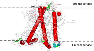
Schematic structural model of CP29 based on the x-ray structure of CP29. The five main helices (A–E) are shown in red. The N-terminus, consisting of residues 1–100, is not defined in the structure. Residue 101 is localized at the stromal surface of the protein, at the start of helix B. To see this figure in color, go online.

The N-terminus is conserved across many species, and the occurrence of phosphorylation sites and the unusual length of the N-terminus in CP29 suggest that its organization is important for the antenna function of CP29. However, it is difficult to model such a long stretch of amino-acid residues without a priori knowledge (19) because input data are necessary to understand its organization and draw conclusions about its function.

Therefore, in this study, we employed spin-label EPR to learn more about the structure and dynamics of the N-terminus. Our study involved two approaches. Singly spin-labeled variants were used to study the rotational diffusion of the spin label by continuous-wave (CW) EPR, and doubly spin-labeled variants were used to determine distances by double electron-electron resonance (DEER), a pulsed EPR method. Amino-acid residues were mutated one by one to a cysteine, spin labeled with a nitroxide spin label (i.e., site-directed spin labeling (SDSL)), and reconstituted with the chlorophylls and carotenoids to form the holoprotein. In all cases, the holoprotein solubilized in β-D-maltoside (DM) was investigated. This study demonstrates that the N-terminus of CP29 is relatively structured and consists of at least five different regions that differ in their secondary structure. We present an attachment-loop-attachment-loop model, show evidence of multiple conformations, and speculate that different conformations could be relevant for the light response of CP29.

Materials and Methods

Mutagenesis, labeling, and pigment reconstitution

The construction and isolation of overexpressed CP29 apoprotein from Lhcb4.1 cDNA of Arabidopsis thaliana (from the Arabidopsis Biological Resource Center DNA Stock Center) were performed as reported previously (8,9). The naturally occurring cysteine (position 108) was replaced by alanine. The mutant protein (C108A) was used to estimate the amount of nonspecific spin labeling (8,9). Single cysteine mutants were introduced at 55 different positions in the N-terminus of the CP29 apoprotein using this template, resulting in the following mutants: G4C, G6C, A10C, A11C, S15C, A16C, T19C, V20C, T21C, T22C, P29C, G30C, A31C, I32C, S33C, G39C, S40C, L41C, V42C, G43C, G46C, F50C, G51C, L52C, G53C, A56C, E57C, Y58C, L59C, Q60C, F61C, S65C, Q68C, N69C, L70C, A71C, N73C, L74C, A75C, G76C, G80C, T81C, T83C, E84C, A85C, A86C, A88C, S90C, T91C, P92C, F93C, Q94C, S97C, G101C, and the wild-type protein, labeled for consistency as C108C.

In the DEER experiments, we investigated three different double cysteine mutants: A56C/S65C, A56C/T81C, and A56C/S97C.

Pigment isolation, labeling, and reconstitution of CP29 pigment complexes were performed as described previously (8,9). Solutions of the spin-labeled CP29 samples were washed and concentrated in sucrose-free DM buffer (0.03% W/V + 10 mM Na₂HPO₄, pH 7.6) just before the EPR measurements were obtained. The integrity of the holoprotein samples was checked by fluorescence excitation and emission measurements, which showed the complete absence of free chlorophylls and carotenoids in all preparations.

CW EPR measurements

Liquid-solution EPR measurements were performed at 279 K on an X-band Bruker Elexsys E-500 EPR system (Bruker, Rheinstetten, Germany) equipped with a super-high-Q cavity ER 4122SHQE in combination with a SuperX X-band microwave bridge type ER 049X. Temperature was controlled with a quartz variable-temperature Dewar inset (Eurotherm, Leesburg, VA). Samples were transferred to 50 μl capillaries and placed in a standard 4-mm quartz EPR tube. Spectra were recorded with 10 mT scan width, a microwave power of 5 mW, a modulation amplitude of 0.1 mT, and a scan time of 82 s. Up to 150 scans were recorded to improve the signal/noise ratio (9).

The frozen-solution EPR measurements were performed at 80 K using an Elexsys E680 spectrometer (Bruker). A rectangular cavity equipped with a helium gas-flow cryostat (Oxford Instruments, Oxfordshire, UK) with an ITC502 temperature controller (Oxford Instruments) was used. For measurements in frozen solution, 3 mm outer diameter quartz tubes were used. To obtain a frozen glass, 20% glycerol was added to the samples before they were frozen in liquid nitrogen. The frozen samples were inserted in the precooled helium gas-flow cryostat. The EPR spectra were recorded using a modulation amplitude of 0.2 mT, a modulation frequency of 100 kHz, and a microwave power of 0.159 mW. The typical accumulation time was 40 min.

Simulation of the CW EPR spectra

Information on the rotational diffusion of the spin label is encoded in the line shape of the EPR spectra (20). In the case of a nonrestricted spin label, the lines are narrow, whereas for a restricted spin label the lines are broad. The spectra were simulated using MATLAB (The MathWorks, Natick, MA) and the EasySpin package (21). All simulations were performed assuming isotropic rotation of the spin label. The spectra were simulated as a superposition of different components, corresponding to fractions of the sample in which spin labels have different rotational diffusion. Attempts to simulate the complex line shapes with anisotropic rotation models rather than with different components were not successful and therefore abandoned. In the remainder of the text, we refer to the rotational diffusion of the spin label as the mobility of the spin label. Each component in a spectrum is defined by the rotation-correlation time, τ_r, of the spin label, and the spectrum is characterized by the τ_r of each fraction and their relative amount. For all components, the following parameters were used: g = [2.00724, 2.00505, 2.00181] (22,23) and A_xx = A_yy = 13 MHz. No absolute calibration of g-values was performed, so the g-tensor parameters are relative. The values used for A_zz for the fast and medium components were the same, but for the slow component a different A_zz value was required (22). This indicates a less polar environment of the spin label in the rotamer that corresponds to the slower rotation-correlation-time component, similar to previous observations (24–27). Overmodulation effects were taken into account in EasySpin. The quality of the agreement between the experimental and simulated lines was checked by visual inspection.

Assessment of the CW EPR spectra

A quick method to define the mobility of the spin label is to determine the characteristic parameters of the spectra according to a previously described approach (28,29–31) in which the inverse of the central line width (ΔB⁻¹, mT⁻¹) (32,33) and the inverse of the second moment (<ΔB²>⁻¹, mT⁻²) (28–31) are used. The more mobile the spin label, the higher are the ΔB⁻¹ and <ΔB²>⁻¹ parameters (32,34).

Parameters to estimate the length of protein regions

To compare the dimensions of the N-terminus, some standard parameters of protein dimensions are used. The distance between two successive C_α atoms, C_αi − C_αi+1, in a protein in the random-coil conformation is reported to be 0.38 nm, assuming that all amide groups are restricted to the trans conformation (35). Thus, if the N-terminus of the CP29 (∼100 amino-acid residues) were completely extended, it would have a length of ∼38 nm. For comparison, the largest dimension of the stromal surface of the CP29 protein is ∼3.2 nm (distance between the farthest two residues e.g., 164–188 or 88–180), which is less than 1/10th of the length of the N-terminus in the extended conformation. Also, the distance from the center of CP29 to the center of the PSII core (8.5 nm) or the center of LHCII (6.5 nm) is too short for a fully extended N-terminus, so the N-terminus is not likely to be in an extended conformation. The distance separating each turn of a helix in the direction of the cylindrical axis is 0.54 nm, which results in a distance of 0.15 nm/residue for the length of the α-helix. For loops, we consider two extreme situations, a fat loop and a thin loop, which are maximally extended horizontally and vertically with respect to the stromal surface, respectively. Assuming a minimal turn diameter of 0.8 nm, the horizontally extended loop has a height of 0.8 nm covering at least two residues at both ends, which leaves for a loop of n_L residues, n_L− 4 residues for the width of the horizontal loop. For the vertically extended loop, the height and width of a loop of n_L residues would be (1/2 × n_L− 2) × 0.38 nm and 0.8 nm, respectively. From these numbers, the length of different sections of the protein can be estimated (see Results).

Pulsed EPR measurements

The DEER measurements were performed at X-band on an Elexsys E680 spectrometer (Bruker) at frequencies of ∼9.3 GHz using a 3 mm split-ring resonator. The temperature was kept at 40 K with helium gas in a CF935 (Oxford Instruments) cryostat with an ITC502 temperature controller (Oxford Instruments). Samples were prepared in 3 mm outer diameter quartz tubes and frozen in liquid nitrogen before insertion into the precooled helium gas-flow cryostat. The pump and observer frequencies were separated by 70 MHz and adjusted as previously described (36). The power of the pump pulse was adjusted to invert the echo maximally (37). The lengths of the pulses at the observer frequency were 16 and 32 ns for the π/2 and π pulses, respectively. The length of the pump pulse was 12 ns. All DEER measurements were performed as two-dimensional experiments to suppress proton modulation (37). The DEER time traces were measured for 10 different τ₁-values spaced by 8 ns starting at τ₁ = 200 ns. The slices were added to obtain hyperfine-modulation-free time traces, which were subsequently analyzed. The typical accumulation time per sample was 16 h. The DEER data were analyzed using the DeerAnalysis program 2011 (38–41), which is available from http://www.epr.ethz.ch/software/index. After background correction of the data using a three-dimensional background, the distance distribution was determined by Tikhonov regularization, with an optimum regularization parameter determined by the L curve criterion (37,38). The significance of features at long distances was checked by the peak-suppression tool, and the shape of the distribution was shown to be independent of the start of the background over a large range of starting times with the validation tool in DeerAnalysis. For easier comparison of the multidistance distributions, Gaussians were fitted to the distributions resulting from Tikhonov regularization.

Results

CW EPR

The CW EPR spectra of the reconstituted holoproteins in the detergent-micelle solution are shown in Fig. 2. The spectra differ substantially from each other. Some of them have particularly broad lines (e.g., the spectra of S33C and G101C). Others have sharp lines (e.g., the spectra of A10C and A86C). As can be seen from the residue numbers, broader lines occur throughout the N-terminus.

Figure 2.

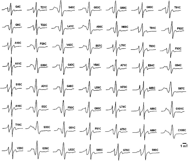
Liquid-solution EPR spectra of 55 singly labeled CP29 protein samples. In each spectrum the position of the nitroxide spin label is indicated.

More detailed information was obtained by spectral simulation performed for selected spectra. For each spectrum (Fig. 3), at least two components are required that differ in rotation-correlation time τ_r (Table 1). The broad-line spectra of the spin label at residues 4, 40, and 101 were simulated with three components. Each spectrum has a substantial slow component (at least 18%) with a τ_r longer than 50 ns, and maximally 5% of a fast component (τ_r = ∼1 ns). In the spectra of the spin label at residues 11 and 86, the slow component is absent, which indicates the more mobile character of these positions. The spectra have almost equal contributions of a fast component with a τ_r of ∼1 ns and a medium component with a τ_r of ∼4 ns. The spectrum of the spin label at residue 70 also consists of two components, except in this case the amount of the medium component (τ_r = ∼4 ns) is significantly larger than that of the fast component (τ_r = ∼1 ns; Table 1).

Figure 3.

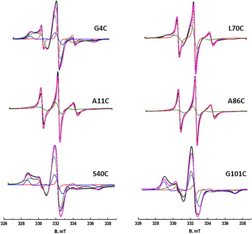
Liquid-solution EPR spectra of singly labeled CP29 at positions 4, 11, 40, 70, 86, and 101. The experimental spectra are shown in black. The simulated spectra are shown in magenta. The simulated spectra are adjusted to fit the intensity in the low-field half of the spectra to account for the asymmetry in the experimental spectra. Each simulated spectrum is a sum of multiple components. The fast, medium, and slow components are shown in red, green, and blue, respectively. To see this figure in color, go online.

Table 1.

EPR parameters derived from simulation of the EPR spectra of singly labeled CP29 proteins

Residue	Fast				Medium				Slow
	τr (ns)	Azz (MHz)	lw (mT)	%	τr (ns)	Azz (MHz)	lw (mT)	%	τr (ns)	Azz (MHz)	lw (mT)	%
G4C	0.67 ± 0.01	109	0.14 ± 0.01	5	4.00 ± 0.10	109	0.32 ± 0.03	77	>50	94	0.60 ± 0.05	18
A11C	1.05 ± 0.01	109	0.08 ± 0.01	47	4.00 ± 0.10	109	0.32 ± 0.03	53	–	–	–	–
S40C	0.83 ± 0.01	109	0.14 ± 0.01	2	4.30 ± 0.10	109	0.32 ± 0.03	78	>50	94	0.60 ± 0.05	20
L70C	0.95 ± 0.01	109	0.08 ± 0.01	26	4.20 ± 0.10	109	0.32 ± 0.03	74	–	–	–	–
A86C	1.05 ± 0.01	109	0.08 ± 0.01	55	4.00 ± 0.10	109	0.32 ± 0.03	45	–	–	–	–
G101C	1.15 ± 0.01	109	0.14 ± 0.01	4	4.30 ± 0.10	109	0.32 ± 0.03	40	>50	94	0.60 ± 0.05	56

A_zz, hyperfine splitting along the z direction; lw, the component line width; %, the contribution of the given component to the total spectrum; τ_r, rotation-correlation time.

Because of the multicomponent character of these spectra, it would be difficult to integrate the individual fitting results of all 55 spectra in a meaningful way; therefore, we used a different approach, the Hubbell plot (29–31,33). It classifies mobility in terms of the location of the residue in the protein (topographic regions), using ΔB⁻¹ (32,33) and <ΔB²>⁻¹. Topographic regions are the loop/surface sites, loop/contact sites, helix/surface sites, and helix/buried sites (28–31,33). For the spin-labeled variants of CP29, the ΔB⁻¹ and <ΔB²>⁻¹ values are shown as blue dots in the Hubbell plot (Fig. 4). This plot also shows the topographic regions as colored areas (33,42). Most points fall within these regions. To relate these points to the sequence, Fig. 5 shows the ΔB⁻¹ and <ΔB²>⁻¹ values and the region color-coding as a function of the sequence number of the residue.

Figure 4.

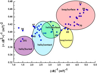
Hubbell plot of the N-terminus of CP29. The values of the inverse second moment, <ΔB²>⁻¹, and the inverse of the central line widths, ΔB⁻¹, of the 55 singly labeled CP29 proteins were determined from the EPR spectra (blue dots). The topological regions of a protein are indicated by ovals according to previous studies (33,42). The color-coded regions represent secondary structure in a protein: red, loop/surface site; yellow, loop/contact site; green, helix/surface site; blue, helix/contact site; and purple, helix/buried site.

Figure 5.

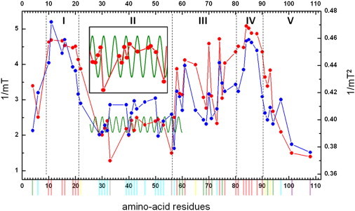
Plot showing the parameters of the Hubbell plot (Fig. 4) as a function of the residue number. The <ΔB²>⁻¹ (blue dots) and ΔB⁻¹ (red dots) values are given. For each amino-acid residue, the color code, which is defined according to the Hubble plot (Fig. 4), is given as a vertical line below the horizontal axis. Different mobility regions are labeled with roman numbers I–V. The superimposed solid green line shows the 3.6 amino-acid periodicity of an α-helix. The inset shows the region between residues 29 and 53 expanded, for better viewing of periodicity.

Ultimately (also including further analysis; see below), five distinct mobility regions are determined within the N-terminus: I, residues 10–22; II, residues 23–57; III, residues 58–81; IV, residues 82–91; and V, residues 92 and 108. Region V includes a stretch of residues (101–108) assigned to the transmembrane helix B, which extends from residue 101 onward. The borders between regions are not precisely defined.

As shown in Fig. 5, the first high-mobility region, region I, fits with the red area in the Hubbell plot, indicating a loop/surface region. The next region with low mobility, region II, falls into the blue area in the Hubbell plot, indicating a helix/contact region. Next is region III, which spreads over the green, red, and yellow areas, indicating a helix/surface and a loop/contact region, respectively. The next high-mobility region, region IV, is mainly in the loop/surface region of the Hubble plot. The last low-mobility region, region V, gradually transits between residues 90 and 97 from flexible to helix surface, to terminate in the helix/buried region in the Hubbell plot. This last section concerns residues close to the transmembrane part of the protein.

We also checked for a possible periodicity in the mobility of sequential residues. Although no part of the sequence exhibits a periodicity of 2, indicative of a β-sheet (33), one stretch of residues (residues 39–46) exhibits a 3.6 periodicity (green line in Fig. 5), which suggests an α-helical stretch. The periodicity for residues 39–46 is most pronounced in the ΔB⁻¹ parameter. This proposed α-helical stretch is projected on an α-helical wheel diagram (see below), which reveals no clear hydrophobicity/hydrophilicity pattern. Several residues on both sides of this helical region also follow the periodicity pattern of a helix (green line in Fig. 5), suggesting that the helix could extend further on either side, potentially extending the helix to residue 29 respectively 53. Clear evidence of periodicity requires data points from several successive residues, and therefore the periodicity between residues 29–38 and 47–53 cannot be confirmed. Since all residues between 29 and 53 are in the helix/contact region of the Hubbell plot, it is likely that the α-helix extends beyond residues 39–46.

Pulsed EPR

Three different intramolecular distances within the N-terminus of the CP29 protein were assessed using pulsed EPR measurements. The DEER time traces show clear nonexponential decays, which differ for all double mutants (Fig. 6 a). The absence of visible modulation indicates multiple distances or broad distance distributions. Distance distributions are obtained by the Tikhonov regularization method (see Materials and Methods). The distance distributions are fitted to a sum of Gaussians, the parameters of which are given in Table 2. Most of the distance distributions are composed of multiple Gaussians (Fig. 6 b), suggesting that the N-terminus adopts several conformations. For all mutants but 56/65, the distributions have at least two components with a distance larger than 2 nm (Table 2). Components with distances below 1.8 nm are disregarded because they cannot be reliably determined under our experimental conditions (40). The presence of very short distances (<1.5 nm) can be excluded from the absence of line broadening in CW EPR spectra (43) of the same mutants (Fig. 6 c).

Figure 6.

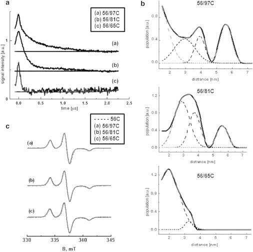
Distance determination of residues within the N-terminus of CP29 for the double mutants 56/65, 56/97, and 56/81. (a) Original DEER traces with the baseline used for correction. (b) Distance distributions obtained by Tikhonov regularization from the data shown in panel a with the corresponding Gaussian fits (performed using Origin Lab software). The experimental curve is shown as a solid line and the sum of the Gaussian contributions is shown as long-dashed lines. (c) CW EPR spectra of the doubly labeled mutants (solid lines) obtained at 80 K superimposed with the spectra of the respective singly labeled counterparts (dashed lines).

Table 2.

Distance parameters for doubly labeled CP29 proteins, derived from analysis of DEER data

Mutant	<r1> nm	S (r1) nm	%	<r2> nm	S (r2) nm	%	<r3> nm	S (r3) nm	%	<r4> nm	S (r4) nm	%
56/65	1.92	1.7	95	1.67	0.6	5	–	–	–	–	–	–
56/81	2.86	1.3	54	3.72	0.9	29	5.62	0.89	17	–	–	–
56/97	1.24	1.51	49	2.95	1.62	21	3.93	0.79	11	5.6	0.9	19

The DEER data were analyzed by means of Tikhonov regularization. The width of the distance distributions reflects the distribution of the conformation of the protein between the spin-label positions, and the conformation distribution of the spin-label linkers. The modulation depths correspond to two coupled spins within a deviation of 12% maximally.

%, the contribution of each peak; <r>, distance in nm; S(r), the width of the distance distribution in nm.

Discussion

We have investigated the N-terminus of CP29 spanning residues 1–110. This part of the protein is often considered to be flexible, and only residues 101–110 are well defined in the x-ray structure (16). Determining the structure of such a flexible and long region of a protein is challenging. To date, the reported algorithms for prediction of loop structures have been applied for loops with 4–20 amino-acid residues only (19,44–46). In this study, 55 out of these 110 residues were selected for single-label sites, providing coverage over the entire region of interest, and three pairs of label positions were chosen to target specifically the regions of residues in the N-terminus of CP29 that have no correspondence with the N-terminus in LHCII.

Comparison of spin-label mobility measures

The mobility of the spin label provides important markers for the structure. Here, we used two different methods to analyze mobility. The most rigorous approach is simulation of the spectra, which reveals the multicomponent nature of the individual spectra. Such multicomponent spectra are often observed in spin-label EPR even for single conformation proteins, where they are attributed to different conformers of the spin-label linker (47). Consequently, the presence of several components in the CW EPR spectra is consistent with (but not sufficient proof of) multiple conformations of the N-terminus. Absolute rotation-correlation times and the relative contribution of each component are obtained. Remarkably, spectra that appear to the eye as immobilized (residues 4 and 40) can have as little as 20% of the slow component, so these spectra appear immobilized due to the presence of a small (≤5%) population of the fast component rather than a large amount of the slow component. The interpretive value of the simulations is limited, however, because the relation of the components and their τ_r values to the structural features of the protein is not yet understood.

A comparison of these parameters with the location in the Hubbell plot (32,33) (Fig. 4) reveals that residues with a slow fraction are located in the helix/buried (residue 101), helix/contact (residue 40), and helix/surface regions (residue 4), emphasizing that these residues are in an area of the protein that restricts their flexibility. Apparently, the amount of slow fraction has a strong impact on the location in the Hubbell plot, as the amount of slow fraction decreases in the order 101, 40, and 4 as well. Residues 4 and 40 also reveal a larger proportion of medium mobility fraction with a rotation-correlation time that is 4.3 ns for residue 40, rather than 4 ns for residue 4, so rather subtle changes in rotation-correlation time and proportion lead to classification in different regions of the Hubbell plot. Residues 11, 70, and 86, all of which are classified as loop/surface in the Hubbell plot, lack the slow fraction and have similar fast and medium rotation-correlation times, albeit in different proportions. In particular, the different locations of residues 11 and 86 in the Hubbell plot reveal the visualization power of the latter method. For these two residues, the simulation parameters are very similar, but nevertheless they are cast on different locations of the plot. The trends of relative amount and rotation-correlation times for the spectra selected for simulation are also seen in the Hubbell approach, confirming the equivalence of both approaches. The advantage of the Hubbell plot is that ample reference data are available, which enables us to classify the residues of the N-terminus according to protein positions.

Three regions of low mobility are identified: the N-terminus itself (residues 4 and 6) and the regions labeled II and V in Fig. 5. A comparison with the Hubbell regions (Fig. 4) reveals that the mobility of the spin label in region II corresponds to those found in the helix/contact regions, those at III to the outer surface of proteins, and those at V (except for the first seven transition residues) to the helix/buried region.

Distances in the N-terminus

The distance measurements show that the N-terminus is not extended. For the nine residues from 56 to 65, for which the fully extended chain would have a length of 3.4 nm, a length of ∼2 nm is found. This compactness is even more evident for the mutant 56/81, which has a major contribution of a distance of 2.9 nm and a minor one of 3.7 nm, whereas the fully extended length would be 9.5 nm. The sequentially even more distant pair of 56/97 has a dominant distance around 3 nm, showing clearly that the N-terminus is compact. The multiple distances found (Table 2) are indicative of multiple conformations of the N-terminus. The widths of the distance distributions are larger than the 0.4–0.5 nm distribution widths typically found for single-conformation proteins acquired with the same spin label (48), another clear indication that the N-terminus is flexible.

Structural features revealed by the EPR results

The N-terminus is relatively structured and certainly not in a completely random, flexible conformation. The first evidence for this comes from the mobility measurements: among the investigated residues (55 out of 110), ∼40% appear to be immobile/restricted, 35% have intermediate mobility, and only 25% are highly mobile. The well-defined distances found by DEER, rather than very broad distance distributions, also show that the probed section of the protein is structured and not random.

There is clear evidence of multiple conformations. The multicomponent nature of the CW EPR spectra is a strong indication; however, spectra with multiple components have also been reported for single-conformation proteins (47). Consequently, the multiple components are suggestive (but not proof) of multiple conformations of the N-terminus. Most clear-cut are the multicomponent distance distributions found in the DEER experiments, which suggest at least two distinct, well-defined conformations.

The N-terminus has several attachment points separated by flexible loops. Immobile, restricted residues are found throughout the N-terminus, indicating multiple attachment points with flexible loops in between.

Relating structural features to the conformation of the N-terminus

Fig. 7 shows how the mobility information relates to structural features of the 100-amino-acid-residue N-terminus. Working our way from residues defined in the x-ray structure toward the end of the N-terminus, residue 101 is located at the stromal end of helix B. It is the first residue known from the x-ray structure. Residue 97 is four residues away from residue 101, so residue 97 must be in a radius of maximally 1.5 nm from the entrance of helix B on the stromal side of the protein. In region IV, residues have a high mobility, which is suggestive of a loop region. Assuming standard parameters for turns and interresidue separation (see Materials and Methods), such a loop can have two extreme shapes: as a flat loop it covers 1.9 nm in width (Fig. 7), and as a long and thin loop it extends 1.3 nm into the stroma. Region III (residues 58–81) has a loop/contact-helix/contact character, so it must be more strongly attached to the protein surface than region IV. In region II, residues 39–46 have a pronounced 3.6 periodicity. The helical wheel projection (Fig. 7, inset) shows that there is no clear hydrophobicity/hydrophilicity pattern in this helix, making it unlikely that it is an amphipathic helix, e.g., a helix bound to the membrane surface. More likely, it interacts with the protein surface. Given that the entire stretch of residues in region II lies in the helix/contact region of the Hubbell plot, it may well be that this helix extends from residues 29–53, corresponding to a total length of the helix of 3.6 nm. Because the latter length is longer than the diagonal extension of the protein’s stromal surface (Fig. 7), the helical stretch probably does not extend as far as residue 53 or it is not a continuous helix. Finally, it is likely that region I, which is flexible and shows no periodicity, is a loop. For region I, a flat loop would cover 3.0 nm, almost traversing the stromal surface of the protein, and as a long and thin loop it would extend 1.9 nm into the stroma, which shows that this loop is longer than the loop in region IV.

Figure 7.

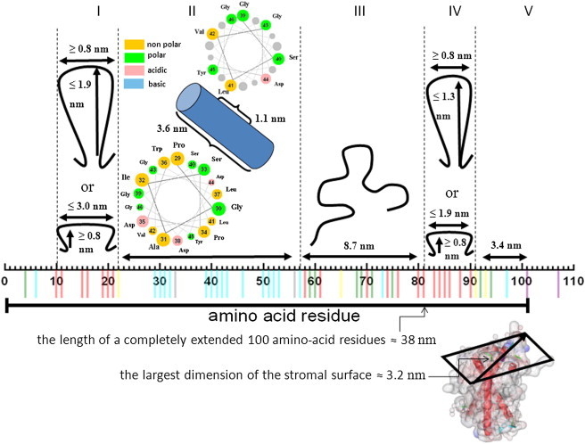
Interpretation of the mobility data obtained by EPR in the single mutants of CP29, giving geometrical constraints for the N-terminus. The residues of the N-terminus are shown horizontally, with colors from the Hubbell plot (Fig. 5). As a reference, the diagonal of the stromal surface is 3.2 nm. The position of residues 101–110 should be close to the stromal surface and helix B. As an extended chain, residues 92–101 would cover a length of 3.4 nm (region V). Different models for the chain conformation result in the lengths shown for regions IV, III, and I (for details, see text). For the two loop regions, dimensions are shown, which the loops would have in two extreme forms: loops that are long and narrow would protrude maximally into the stroma, whereas wide and flat loops would be more close to the protein surface. The dimensions were calculated assuming a minimum turn diameter of 8 Å. Region II can be an α-helix. Helical-wheel diagram for region II with the corresponding amino-acid residues are depicted in colors. The color codes represent the type of amino-acid residues in the helical wheel. The numbers on each circle refer to the number of the residue within the N-terminus. Going down the helix, the size of the circles representing the residues in the helical wheel decreases (http://cti.itc.Virginia.EDU/∼cmg/Demo/wheel/wheelApp.html).

The overall architecture reveals noncovalent attachment of several N-terminal residues (at least residues 4–6), the middle part of the N-terminus (residues 39–46), and the end of the N-terminus (from residue 100 onward). Two flexible regions (I and IV) flank a less flexible region. The N-terminal part of the protein is located on the stromal side of the protein, which suggests that the less mobile regions are embedded in the stromal surface of the protein.

Our first conclusion is that the N-terminus, which in its fully extended form would have a length of 38 nm, is surprisingly structured. It loops back and forth on the stromal surface of the protein.

The presence of multiple conformations of the N-terminus, as concluded from our EPR investigation, is in agreement with the heterogeneity reported in previous studies (8,9). These studies described two loop regions, a short one and a longer one, that either stick out into the stroma (9) or lie flat on the hydrophobic core most of the time (8). According to these EPR and FRET studies (8,9), residue 15 is part of the short loop, and residues 65, 82, and 90 belong to the long loop. Similarly to those previous reports, we find two loops. We further differentiate the reported long-loop region (8,9) into two mobility sections (regions III and IV), rather than one continuous mobility section. So, essentially the long loop described by Berghuis et al. (8) and Kavalenka et al. (9) becomes our short loop, containing both phosphorylation sites (14). In contrast to the previous EPR study, around residue 65 we find several residues of lower mobility (residues 57, 59, 60, 68, 69, 71, 73, and 75), arguing that residues 58–81 do not form part of the loop, although residue 65 has a relatively high mobility. Therefore, in addition to the report of Kavalenka et al. (9), in which 10 residues of the N-terminus were investigated, a lot of information can be resolved by characterizing the 55 residues we have studied here. The structure of residues 58–97 is particularly relevant because these residues are only present in CP29, and not in LHCII, which otherwise is similar to CP29. This may help to explain the difference in function of CP29 and LHCII in the outer membrane antenna complex.

Summary and Conclusions

This study demonstrates that the N-terminus of CP29 is relatively structured and is separated into regions with strongly differing mobilities. Moreover, there are clear signs of heterogeneity, demonstrating that the N-terminus is not fixed in one particular structure, but is able to adopt various conformations. The presence of phosphorylation sites that are affected by light conditions in this region of the protein (e.g., at positions 81 and 83 (14)) is a strong indication that the N-terminus is important in membrane organization. The flexibility of the N-terminus found here may be functionally important because it enables the N-terminus to switch between different conformations, thereby allowing the system to adapt to different environmental (light) conditions.

We speculate that the combination of loops and attachment points provides a sufficient structural scaffold to enable specific interactions with other membrane components. Flexible sections could serve to anchor CP29 to other antenna proteins. However, by limiting the number of attachment points, static structures and low energetic minima are avoided, thus enabling transitions to a limited number of alternative conformations. We hypothesize that the balance between these conformations could be affected by phosphorylation, providing the means to enable CP29 to respond to different light conditions.

References

- 1.Croce R., van Amerongen H. Light-harvesting and structural organization of Photosystem II: from individual complexes to thylakoid membrane. J. Photochem. Photobiol. B. 2011;104:142–153. doi: 10.1016/j.jphotobiol.2011.02.015. [DOI] [PubMed] [Google Scholar]
- 2.Scholes G.D., Fleming G.R., van Grondelle R. Lessons from nature about solar light harvesting. Nat. Chem. 2011;3:763–774. doi: 10.1038/nchem.1145. [DOI] [PubMed] [Google Scholar]
- 3.Caffarri S., Kouril R., Croce R. Functional architecture of higher plant photosystem II supercomplexes. EMBO J. 2009;28:3052–3063. doi: 10.1038/emboj.2009.232. [DOI] [PMC free article] [PubMed] [Google Scholar]
- 4.Caffarri S., Broess K., van Amerongen H. Excitation energy transfer and trapping in higher plant Photosystem II complexes with different antenna sizes. Biophys. J. 2011;100:2094–2103. doi: 10.1016/j.bpj.2011.03.049. [DOI] [PMC free article] [PubMed] [Google Scholar]
- 5.Ahn T.K., Avenson T.J., Fleming G.R. Architecture of a charge-transfer state regulating light harvesting in a plant antenna protein. Science. 2008;320:794–797. doi: 10.1126/science.1154800. [DOI] [PubMed] [Google Scholar]
- 6.Ginsberg N.S., Davis J.A., Fleming G.R. Solving structure in the CP29 light harvesting complex with polarization-phased 2D electronic spectroscopy. Proc. Natl. Acad. Sci. USA. 2011;108:3848–3853. doi: 10.1073/pnas.1012054108. [DOI] [PMC free article] [PubMed] [Google Scholar]
- 7.Mauro S., Dainese P., Bassi R. Cold-resistant and cold-sensitive maize lines differ in the phosphorylation of the photosystem II subunit, CP29. Plant Physiol. 1997;115:171–180. doi: 10.1104/pp.115.1.171. [DOI] [PMC free article] [PubMed] [Google Scholar]
- 8.Berghuis B.A., Spruijt R.B., van Amerongen H. Exploring the structure of the N-terminal domain of CP29 with ultrafast fluorescence spectroscopy. Eur. Biophys. J. 2010;39:631–638. doi: 10.1007/s00249-009-0519-9. [DOI] [PMC free article] [PubMed] [Google Scholar]
- 9.Kavalenka A.A., Spruijt R.B., van Amerongen H. Site-directed spin-labeling study of the light-harvesting complex CP29. Biophys. J. 2009;96:3620–3628. doi: 10.1016/j.bpj.2009.01.038. [DOI] [PMC free article] [PubMed] [Google Scholar]
- 10.van Oort B., Murali S., van Amerongen H. Ultrafast resonance energy transfer from a site-specifically attached fluorescent chromophore reveals the folding of the N-terminal domain of CP29. Chem. Phys. 2009;357:113–119. [Google Scholar]
- 11.Mozzo M., Passarini F., Croce R. Photoprotection in higher plants: the putative quenching site is conserved in all outer light-harvesting complexes of Photosystem II. Biochim. Biophys. Acta. 2008;1777:1263–1267. doi: 10.1016/j.bbabio.2008.04.036. [DOI] [PubMed] [Google Scholar]
- 12.Chen Y.E., Zhao Z.Y., Yuan S. The significance of CP29 reversible phosphorylation in thylakoids of higher plants under environmental stresses. J. Exp. Bot. 2013;64:1167–1178. doi: 10.1093/jxb/ert002. [DOI] [PubMed] [Google Scholar]
- 13.Pascal A., Gradinaru C., van Amerongen H. Spectroscopic characterization of the spinach Lhcb4 protein (CP29), a minor light-harvesting complex of photosystem II. Eur. J. Biochem. 1999;262:817–823. doi: 10.1046/j.1432-1327.1999.00457.x. [DOI] [PubMed] [Google Scholar]
- 14.Fristedt R., Vener A.V. High light induced disassembly of photosystem II supercomplexes in Arabidopsis requires STN7-dependent phosphorylation of CP29. PLoS ONE. 2011;6:e24565. doi: 10.1371/journal.pone.0024565. [DOI] [PMC free article] [PubMed] [Google Scholar]
- 15.Croce R., Breton J., Bassi R. Conformational changes induced by phosphorylation in the CP29 subunit of photosystem II. Biochemistry. 1996;35:11142–11148. doi: 10.1021/bi960652t. [DOI] [PubMed] [Google Scholar]
- 16.Pan X., Li M., Chang W. Structural insights into energy regulation of light-harvesting complex CP29 from spinach. Nat. Struct. Mol. Biol. 2011;18:309–315. doi: 10.1038/nsmb.2008. [DOI] [PubMed] [Google Scholar]
- 17.Jansson S. A guide to the Lhc genes and their relatives in Arabidopsis. Trends Plant Sci. 1999;4:236–240. doi: 10.1016/s1360-1385(99)01419-3. [DOI] [PubMed] [Google Scholar]
- 18.Dockter C., Volkov A., Paulsen H. Refolding of the integral membrane protein light-harvesting complex II monitored by pulse EPR. Proc. Natl. Acad. Sci. USA. 2009;106:18485–18490. doi: 10.1073/pnas.0906462106. [DOI] [PMC free article] [PubMed] [Google Scholar]
- 19.Subramani A., Floudas C.A. Structure prediction of loops with fixed and flexible stems. J. Phys. Chem. B. 2012;116:6670–6682. doi: 10.1021/jp2113957. [DOI] [PMC free article] [PubMed] [Google Scholar]
- 20.Steinhoff H.J. A simple method for determination of rotational correlation times and separation of rotational and polarity effects from EPR spectra of spin-labeled biomolecules in a wide correlation time range. J. Biochem. Biophys. Methods. 1988;17:237–247. doi: 10.1016/0165-022x(88)90047-4. [DOI] [PubMed] [Google Scholar]
- 21.Stoll S., Schweiger A. EasySpin, a comprehensive software package for spectral simulation and analysis in EPR. J. Magn. Reson. 2006;178:42–55. doi: 10.1016/j.jmr.2005.08.013. [DOI] [PubMed] [Google Scholar]
- 22.Sepkhanova I., Drescher M., Huber M. Monitoring Alzheimer amyloid peptide aggregation by EPR. Appl. Magn. Reson. 2009;36:209–222. doi: 10.1007/s00723-009-0019-1. [DOI] [PMC free article] [PubMed] [Google Scholar]
- 23.Shabestari M., Plug T., Huber M. The aggregation potential of the 1–15- and 1–16-fragments of the amyloid β peptide and their influence on the aggregation of Aβ40. Appl. Magn. Reson. 2013;44:1167–1179. [Google Scholar]
- 24.Owenius R., Osterlund M., Carlsson U. Spin and fluorescent probing of the binding interface between tissue factor and factor VIIa at multiple sites. Biophys. J. 2001;81:2357–2369. doi: 10.1016/S0006-3495(01)75882-1. [DOI] [PMC free article] [PubMed] [Google Scholar]
- 25.Hammarström P., Owenius R., Lindgren M. High-resolution probing of local conformational changes in proteins by the use of multiple labeling: unfolding and self-assembly of human carbonic anhydrase II monitored by spin, fluorescent, and chemical reactivity probes. Biophys. J. 2001;80:2867–2885. doi: 10.1016/S0006-3495(01)76253-4. [DOI] [PMC free article] [PubMed] [Google Scholar]
- 26.Hammarström P., Persson M., Carlsson U. Protein substrate binding induces conformational changes in the chaperonin GroEL. A suggested mechanism for unfoldase activity. J. Biol. Chem. 2000;275:22832–22838. doi: 10.1074/jbc.M000649200. [DOI] [PubMed] [Google Scholar]
- 27.Owenius R., Osterlund M., Carlsson U. Properties of spin and fluorescent labels at a receptor-ligand interface. Biophys. J. 1999;77:2237–2250. doi: 10.1016/S0006-3495(99)77064-5. [DOI] [PMC free article] [PubMed] [Google Scholar]
- 28.Van Vleck J.H. The dipolar broadening of magnetic resonance lines in crystals. Phys. Rev. 1948;74:1168–1183. [Google Scholar]
- 29.Hubbell W.L., Altenbach C. Investigation of structure and dynamics in membrane proteins using site-directed spin labeling. Curr. Opin. Struct. Biol. 1994;4:566–573. [Google Scholar]
- 30.Mchaourab H.S., Lietzow M.A., Hubbell W.L. Motion of spin-labeled side chains in T4 lysozyme. Correlation with protein structure and dynamics. Biochemistry. 1996;35:7692–7704. doi: 10.1021/bi960482k. [DOI] [PubMed] [Google Scholar]
- 31.Mchaourab H.S., Kálai T., Hubbell W.L. Motion of spin-labeled side chains in T4 lysozyme: effect of side chain structure. Biochemistry. 1999;38:2947–2955. doi: 10.1021/bi9826310. [DOI] [PubMed] [Google Scholar]
- 32.Oda M.N., Forte T.M., Voss J.C. The C-terminal domain of apolipoprotein A-I contains a lipid-sensitive conformational trigger. Nat. Struct. Biol. 2003;10:455–460. doi: 10.1038/nsb931. [DOI] [PubMed] [Google Scholar]
- 33.Hubbell W.L., Mchaourab H.S., Lietzow M.A. Watching proteins move using site-directed spin labeling. Structure. 1996;4:779–783. doi: 10.1016/s0969-2126(96)00085-8. [DOI] [PubMed] [Google Scholar]
- 34.Columbus L., Hubbell W.L. A new spin on protein dynamics. Trends Biochem. Sci. 2002;27:288–295. doi: 10.1016/s0968-0004(02)02095-9. [DOI] [PubMed] [Google Scholar]
- 35.Miller W.G., Goebel C.V. Dimensions of protein random coils. Biochemistry. 1968;7:3925–3935. doi: 10.1021/bi00851a021. [DOI] [PubMed] [Google Scholar]
- 36.Drescher M., Veldhuis G., Huber M. Antiparallel arrangement of the helices of vesicle-bound α-synuclein. J. Am. Chem. Soc. 2008;130:7796–7797. doi: 10.1021/ja801594s. [DOI] [PubMed] [Google Scholar]
- 37.Jeschke G. Distance measurements in the nanometer range by pulse EPR. ChemPhysChem. 2002;3:927–932. doi: 10.1002/1439-7641(20021115)3:11<927::AID-CPHC927>3.0.CO;2-Q. [DOI] [PubMed] [Google Scholar]
- 38.Jeschke G., Chechik V., Jung H. DeerAnalysis2006—a comprehensive software package for analyzing pulsed ELDOR data. Appl. Magn. Reson. 2006;30:473–498. [Google Scholar]
- 39.Jeschke G., Panek G., Paulsen H. Data analysis procedures for pulse ELDOR measurements of broad distance distributions. Appl. Magn. Reson. 2004;26:223–244. [Google Scholar]
- 40.Jeschke G., Polyhach Y. Distance measurements on spin-labelled biomacromolecules by pulsed electron paramagnetic resonance. Phys. Chem. Chem. Phys. 2007;9:1895–1910. doi: 10.1039/b614920k. [DOI] [PubMed] [Google Scholar]
- 41.Jeschke G. DEER distance measurements on proteins. Annu. Rev. Phys. Chem. 2012;63:419–446. doi: 10.1146/annurev-physchem-032511-143716. [DOI] [PubMed] [Google Scholar]
- 42.Isas J.M., Langen R., Hubbell W.L. Structure and dynamics of a helical hairpin and loop region in annexin 12: a site-directed spin labeling study. Biochemistry. 2002;41:1464–1473. doi: 10.1021/bi011856z. [DOI] [PubMed] [Google Scholar]
- 43.Robotta M., Braun P., Drescher M. Direct evidence of coexisting horseshoe and extended helix conformations of membrane-bound α-synuclein. ChemPhysChem. 2011;12:267–269. doi: 10.1002/cphc.201000815. [DOI] [PubMed] [Google Scholar]
- 44.Subramaniam R., Koppal T., Butterfield D.A. The free radical antioxidant vitamin E protects cortical synaptosomal membranes from amyloid β-peptide(25-35) toxicity but not from hydroxynonenal toxicity: relevance to the free radical hypothesis of Alzheimer’s disease. Neurochem. Res. 1998;23:1403–1410. doi: 10.1023/a:1020754807671. [DOI] [PubMed] [Google Scholar]
- 45.Floudas C.A., Fung H.K., Rajgaria R. Advances in protein structure prediction and de novo protein design: a review. Chem. Eng. Sci. 2006;61:966–988. [Google Scholar]
- 46.Floudas C.A. Computational methods in protein structure prediction. Biotechnol. Bioeng. 2007;97:207–213. doi: 10.1002/bit.21411. [DOI] [PubMed] [Google Scholar]
- 47.Steinhoff H.J. Methods for study of protein dynamics and protein-protein interaction in protein-ubiquitination by electron paramagnetic resonance spectroscopy. Front. Biosci. 2002;7:c97–c110. doi: 10.2741/A763. [DOI] [PubMed] [Google Scholar]
- 48.Finiguerra M.G., Prudêncio M., Huber M. Accurate long-range distance measurements in a doubly spin-labeled protein by a four-pulse, double electron-electron resonance method. Magn. Reson. Chem. 2008;46:1096–1101. doi: 10.1002/mrc.2290. [DOI] [PubMed] [Google Scholar]