SENSE Phase-Constrained Magnitude Reconstruction With Iterative Phase Refinement

Abstract

Conventional sensitivity encoding (SENSE) reconstruction is based on equations in the complex domain. However, for many MRI applications only the magnitude is relevant. If there exists an estimate of the underlying phase information, a magnitude-only phase-constrained reconstruction can help to improve the conditioning of the SENSE reconstruction problem. Consequently, this reduces g-factor-related noise enhancement. In previous attempts at phase-constrained SENSE reconstruction, image quality was hampered by strong aliasing artifacts resulting from inadequate phase estimates and high sensitivity to phase errors. If a full-resolution phase image is used, a significant reduction in aliasing errors and better noise properties compared to SENSE can be obtained. An iterative scheme that improves the phase estimate to better approximate the phase is presented. The mathematical framework of the new approach is provided together with comparisons of conventional SENSE, phase-constrained SENSE, and the new phase-refinement method. Both theory and experimental verification demonstrate significantly better noise performance at high reduction factors, i.e., close to the theoretical limit. For applications that need only magnitude data, an iterative phase-constrained SENSE reconstruction can provide substantial SNR improvement over SENSE reconstruction and less artifacts than phase-constrained SENSE.

The advent of parallel imaging in magnetic resonance imaging (MRI) has opened a door for collecting data using less time. Parallel imaging allows applications such as phase contrast imaging (1), cine imaging (2), fast spin echo (FSE) (3), and diffusion-weighted imaging (DWI) (4,5) to be completed faster to avoid subjecting patients to long scan times and to reduce artifacts. It can alternatively improve the temporal resolution by reducing the amount of views per segment, as in a cine acquisition (6). Sensitivity encoding (SENSE) (7) is one realization of parallel imaging. It can be thought of intuitively as a method of solving the inverse imaging problem as an overdetermined system of equations using the coil sensitivity profiles as linear weights and an undersampled set of pixels as the measured data. These equations typically operate on complex numbers, and the reconstruction yields an estimate of the underlying image in a minimum least-squares sense.

In a larger number of MR applications, only the magnitude of an image is of concern. Numerous methods have been developed that improve the signal-to-noise ratio (SNR) or reduce the number of phase encodes by exploiting the need for magnitude-only reconstruction. Homodyne reconstruction (8) is a method that exploits the inherent “realness” of the subject to be imaged, and uses a low-resolution phase estimate to correct for phase discrepancies that occur from the acquisition of the k-space data. Projection onto convex sets (POCS) (9–11) builds on the homodyne method by iterating on the initial reconstruction and filling in the missing k-space samples while concurrently constraining the datasets.

Recent works have combined the idea of both parallel imaging and partial Fourier techniques. The effects of combining SENSE with partial Fourier techniques that employ the POCS and homodyne reconstruction methods have been explored (12). In addition, POCSENSE (13), which uses POCS as an alternative method to reconstruct images acquired with parallel imaging, has been proposed. POCSENSE has the flexibility to incorporate partial Fourier sampling.

Some initial investigations (13–17) have explored the use of phase-constrained reconstruction. Here, an estimate of the underlying image phase is used to improve the SENSE reconstruction. The number of unknowns in the SENSE system of equations is reduced by half, and therefore the overdetermination of the system of equations increases. The g-factor intuitively decreases and leads to less g-factor noise amplification.

In general, it can be assumed that the phase of an image varies smoothly in space. Off-resonance, B₁ inhomogeneity, and eddy currents are examples of sources that cause these phases. However, certain abrupt phase transitions may occur at air–tissue or lipid–tissue interfaces that violate the phase-constraint condition, an observation also known in partial Fourier imaging. Similarly, phase-constrained reconstruction suffers from a lack of high-spatial frequency information regarding the phase in an image, and consequently may suffer from residual aliasing in these regions. We introduce a variant of phase-constrained SENSE, termed “turboSENSE” (18,19), that aims to 1) recover the high spatial frequencies of the phase, 2) eliminate the aliasing artifacts by means of an iterative algorithm, and 3) minimize the g-factor-related noise enhancement. Specifically, a method to improve the phase estimate that was recently introduced for multicoil Dixon chemical species separation is adapted (20). The algorithm assumes that the residual error norm as a function of phase of the aliased pixels follows a smooth convex distribution, and follows an iterative conjugate-gradient method.

It is anticipated that the method can be applied to the many facets of MRI in which only magnitude data are needed. In the following sections, the mathematical framework of turboSENSE and the corresponding iterative algorithm for improving the phase estimate are provided. Our theory was experimentally verified in phantom measurements as well as cardiac and brain scans.

THEORY

Phase-Constrained SENSE Review

In Cartesian SENSE, an undersampled set of k-space data is collected across a multichannel receiver set. Specifically, the acquisition can be represented by the following:

$$\mathbf{s}=\mathbf{C}\mathbf{\rho }+\epsilon$$ [1]

where s is an (N_kN_c) × 1 vector representing the acquired dataset in k-space for a set of N_c coils and N_k k-space samples, C is an N_kN_c × N² complex matrix representing the coil sensitivities and Fourier kernel for an image of N × N pixels, ε is an (N_kN_c) × 1 complex vector representing independent measurement noise, and ρ represents the unaliased complex magnetization for a set of N² pixels. Equation [1] represents a system of equations with N² complex unknowns and N_kN_c complex equations for a total of 2N² real unknowns and 2N_kN_c real equations. The complex reconstruction can be estimated in a minimum least-squares sense, i.e., min(||Cρ^recon − s||), leading to ρ^recon − (C^HΨ⁻¹C)⁻¹C^HΨ⁻¹s, where Ψ represents the noise covariance matrix (7).

Suppose now that only the magnitude is of interest. The magnitude and phase of the unaliased magnetization can be expressed by ρ = diag(exp(iϕ))ρ^mag, where diag(exp(iϕ)) is an N² × N² diagonal matrix whose diagonal elements represent the phase, and ρ^mag is an N² × 1 vector that represents the magnitude of each voxel. Without loss of generality, ρ^mag is a real quantity. We let ρ^mag = Re(ρ^mag). Thus, the SENSE acquisition (Eq. [1]) can now be expressed as:

$$\mathbf{s}=\mathbf{C}\text{diag}(exp(i\varphi ))Re({\mathbf{\rho }}^{\mathit{mag}})+\epsilon ,$$ [2a]

Equation [2a] is then split into real and imaginary components:

$$\left[\begin{array}{c}Re(\mathbf{s})\\ Im(\mathbf{s})\end{array}\right]=\left[\begin{array}{c}Re(\mathbf{C}\text{diag}(exp(i\varphi )))\\ Im(\mathbf{C}\text{diag}(exp(i\varphi )))\end{array}\right]Re({\mathbf{\rho }}^{\mathit{mag}})+\left[\begin{array}{c}Re(\epsilon )\\ Im(\epsilon )\end{array}\right]$$ [2b]

In the phase-constrained formalism, this phase is estimated and can be represented by diag(exp(iϕ)) ≈ diag (exp(iϕ̂)). This phase can be estimated by incorporating the phase present in the scan used to estimate the coil sensitivities. The coil sensitivities can be estimated by many means, such as with a separate calibration scan or the central phase encodes of an autocalibrated scan.

With a perfect phase estimate, we arrive at:

$$\left[\begin{array}{c}Re(\mathbf{s})\\ Im(\mathbf{s})\end{array}\right]=\left[\begin{array}{c}Re(\mathbf{C}\text{diag}(exp(i\widehat{\varphi })))\\ Im(\mathbf{C}\hspace{0.17em}\text{diag}(exp(i\widehat{\varphi })))\end{array}\right]Re({\mathbf{\rho }}^{\mathit{mag}})+\left[\begin{array}{c}Re(\epsilon )\\ Im(\epsilon )\end{array}\right],$$ [3a]

or

$${\mathbf{s}}^{pc}={\mathbf{C}}^{pc}{\mathbf{\rho }}^{pc}+{\epsilon }^{pc}.$$ [3b]

where

$${\mathbf{s}}^{pc}=\left[\begin{array}{c}Re(\mathbf{s})\\ Im(\mathbf{s})\end{array}\right],{\mathbf{C}}^{pc}=\left[\begin{array}{c}Re(\mathbf{C}\text{diag}(exp(i\widehat{\varphi })))\\ Im(\mathbf{C}\text{diag}(exp(i\widehat{\varphi })))\end{array}\right],{\mathbf{\rho }}^{pc}=Re({\mathbf{\rho }}^{\mathit{mag}}),\text{and}{\epsilon }^{pc}=\left[\begin{array}{c}Re(\epsilon )\\ Im(\epsilon )\end{array}\right].$$

Equation [3b] represents the phase-constrained formalism as explained in Ref. 15. With an assumption that the real and imaginary parts are linearly independent, the phase-constrained formulation is now a system of equations with 2N_kN_c equations and N² unknowns. The reconstruction, ρ^pc,recon, can be estimated in a minimum least-squares sense: ρ^pc,recon = (C^pcHΨ^pc−1C^pc)−1C^pcHΨ^pc−1s^pc. The phase-constrained formalism is based on the idea that with an excellent phase estimate, only the real component of the magnetization remains to be computed.

Phase Errors

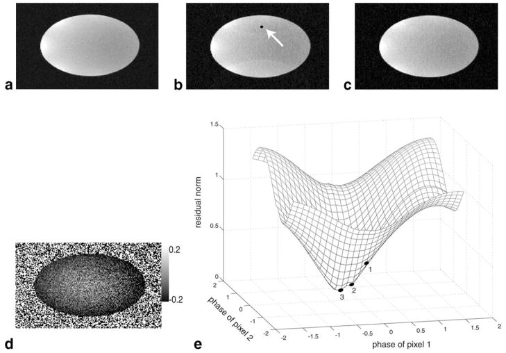
In reality, diag(exp(iϕ̂)) is not a perfect estimate. Figure 1 shows the effect of applying a phase-constrained SENSE reconstruction to a water phantom. The phantom data were acquired twice. The data from the first scan were used to compute the coil sensitivities for an undersampled set of the second scan. The coil sensitivities were calculated by normalizing the surface coil images by the square root of the sum-of-squares. An error in the phase estimate can arise from phase mismatches between the calibration scan and the undersampled acquisition. In addition, although the object itself is smooth, there normally exist some transient phases at the boundary between object and background. Figure 1d shows the phase difference between the two acquisitions, where phase mismatches and transient effects are present. Errors in phase estimates can also arise at boundaries between water and fat, where high spatial frequencies are insufficiently sampled by the phase estimate.

FIG. 1.

Phase-constrained magnitude-only SENSE reconstruction is very sensitive to phase errors in the coil sensitivity maps. a: Reference image of a fully-resolved water phantom. b: Phase-constrained SENSE reconstruction at R = 2. The sensitivity map was obtained from a separate scan with identical parameters. Clearly, a mismatch between the phase of the calibration scan and the undersampled scan is seen as residual aliasing at the reconstruction. c: TurboSENSE reconstruction with iterative phase refinement. The aliasing has been reduced considerably. The black point is a set of two aliased pixels. d: Phase difference between the two separate scans, scaled to display from − 0.2 to 0.2 radians. e: A residual norm surface as a function of different phases applied to the two aliased pixels. The numbers indicate the trajectory taken by the turboSENSE reconstruction during three iterations.

We model this error by introducing an error term to the phase-constrained formalism:

$$\left[\begin{array}{c}Re(\mathbf{s})\\ Im(\mathbf{s})\end{array}\right]=\left[\begin{array}{c}Re(\mathbf{C}\text{diag}(exp(i\widehat{\varphi })))\\ Im(\mathbf{C}\hspace{0.17em}\text{diag}(exp(i\widehat{\varphi })))\end{array}\right]Re({\mathbf{\rho }}^{\mathit{mag}})+\delta +\left[\begin{array}{c}Re(\epsilon )\\ Im(\epsilon )\end{array}\right]$$ [4]

Because the phase estimate has errors, the magnitude of the magnetization ρ^mag will be composed of both a real and an imaginary part. In fact,

$$\delta =\left[\begin{array}{c}-Im(\mathbf{C}\text{diag}(exp(i\widehat{\varphi })))\\ Re(\mathbf{C}\text{diag}(exp(i\widehat{\varphi })))\end{array}\right]Im({\mathbf{\rho }}^{\mathit{mag}}).$$

This term is obtained by inferring from a non-phase-constrained acquisition:

$$\left[\begin{array}{c}Re(\mathbf{s})\\ Im(\mathbf{s})\end{array}\right]=\left[\begin{array}{cc}Re(\mathbf{C}\text{dg}(exp(i\widehat{\varphi })))& -Im(\mathbf{C}\text{dg}(exp(i\widehat{\varphi })))\\ Im(\mathbf{C}\text{dg}(exp(i\widehat{\varphi })))& Re(\mathbf{C}\text{dg}(exp(i\widehat{\varphi })))\end{array}\right]\times \left[\begin{array}{c}Re({\mathbf{\rho }}^{\mathit{mag}})\\ Im({\mathbf{\rho }}^{\mathit{mag}})\end{array}\right]$$ [5]

The error term can be assumed to have a finite mean and variance, ${\sigma }_{\delta }^2$. The variance in the reconstruction, σ², is related to the error by:

$${\sigma }_k^2={\sigma }_{\delta }^2{({\mathbf{C}}^{{pc}^H}{\mathbf{C}}^{pc})}_k^{-1}$$ [6]

for the kth diagonal element (21). ${({\mathbf{C}}^{{pc}^H}{\mathbf{C}}^{pc})}_k^{-1}$ can be used as a measure of the noise amplification since it shows on average the increase in the variance.

TurboSENSE

TurboSENSE aims to reduce the reconstruction error by improving the phase estimate. If we know the phase mismatch, then we can adjust the phase in Eq. [3] and reestimate the reconstruction in the minimum least-squares sense.

To correct for the phase mismatch, we introduce an approach that was previously used to estimate field-map inhomogeneity in multipoint Dixon imaging (20). It is based on an iterative refinement of the phase estimate so that the norm of the residual error, which we call the residual norm, of Eq. [3] becomes a minimum. Figure 1e shows the residual norm as a function of ϕ̂ for the simple case of two aliased pixels. We note that the residual norm has a local minimum, and the initial phase-constrained SENSE reconstruction is not at the minimum. It is hypothesized that the combination of phases ϕ̂ to minimize the residual norm will produce a reconstruction that minimizes residual aliasing artifacts. Specifically, we define the residual error

$$\mathrm{\Delta }{\mathbf{s}}^{pc}={\mathbf{s}}^{pc}-{\mathbf{C}}^{pc}{\mathbf{\rho }}^{pc,\mathit{recon}},$$ [7]

which can be also can be expressed as the first-order differential:

$$\mathrm{\Delta }{\mathbf{s}}^{pc}=\sum _j\left(\frac{\partial {\mathbf{s}}^{pc}}{\partial {\rho }_j^{\mathit{mag}}}\right)\mathrm{\Delta }{\rho }_j^{\mathit{mag}}+\sum _j\left(\frac{\partial {\mathbf{s}}^{pc}}{\partial {\varphi }_j}\right)\mathrm{\Delta }{\varphi }_j$$ [8]

where Δϕ_j is the phase error of the jth pixel, and $\mathrm{\Delta }{\rho }_j^{\mathit{mag}}$ is the magnitude error. To find the derivative in Eq. [8], we return to Eq. [1] and expand the kth k-space sampling point in s:

$$s_k=\sum _j{C}_{kj}exp(i{\varphi }_j){\rho }_j^{\mathit{mag}}$$ [9]

Taking the derivative of Eq. [9] with respect to ϕ_j and ${\rho }_j^{\mathit{mag}}$, we arrive at:

$${ds}_k=\sum _j{C}_{kj}d(exp(i{\varphi }_j){\rho }_j^{\mathit{mag}})$$ [10a]

$${ds}_k=\sum _j{C}_{kj}\left(\frac{\partial }{\partial {\rho }_j^{\mathit{mag}}}(exp(i{\varphi }_j){\rho }_j^{\mathit{mag}}){d\rho }_j^{\mathit{mag}}+\frac{\partial }{\partial {\varphi }_j}(exp(i{\varphi }_j){\rho }_j^{\mathit{mag}})d{\varphi }_j\right)$$ [10b]

$${ds}_k=\sum _j{C}_{kj}(exp(i{\varphi }_j){d\rho }_j^{\mathit{mag}}+i\text{exp}(i{\varphi }_j){\rho }_j^{\mathit{mag}}d{\varphi }_j)$$ [10c]

$$\mathrm{\Delta }{s}_k\approx \sum _j{C}_{kj}(exp(i{\varphi }_j)\mathrm{\Delta }{\rho }_j^{\mathit{mag}}+i\text{exp}(i{\varphi }_i){\rho }_j^{\mathit{mag}}\mathrm{\Delta }{\varphi }_j)$$ [10d]

Equation [10] can be generalized into a matrix equation:

$$\mathrm{\Delta }\mathbf{s}=\mathbf{\Delta }\mathbf{C}\mathbf{\Delta }\mathbf{\rho }$$ [11]

with the elements as follows:

$$\begin{array}{c}\mathrm{\Delta }\text{s}={[\begin{array}{cccc}\mathrm{\Delta }{s}_1& \mathrm{\Delta }{s}_1& \cdots & \mathrm{\Delta }{s}_{\mathit{NkNc}}\end{array}]}^T,\mathrm{\Delta }\mathbf{\rho }={[\begin{array}{cccccc}\mathrm{\Delta }{\rho }_1^{\mathit{mag}}& \cdots & \mathrm{\Delta }{\rho }_{N^2}^{\mathit{mag}}& \mathrm{\Delta }{\varphi }_1& \cdots & \mathrm{\Delta }{\varphi }_{N^2}\end{array}]}^T\\ \mathrm{\Delta }\mathbf{C}=\left[\begin{array}{cccccc}{C}_{1,1}exp(i{\varphi }_1)& \cdots & C_{1,N^2}exp(i{\varphi }_{N^2})& C_{1,1}i\text{exp}(i{\varphi }_1){\rho }_1^{\mathit{mag}}& \cdots & C_{1,N^2}i\text{exp}(i{\varphi }_{N^2}){\rho }_{N^2}^{\mathit{mag}}\\ ⋮& \ddots & ⋮& ⋮& \ddots & ⋮\\ C{\{}_{N_k{N}_c}\},1exp(i{\varphi }_1)& \cdots & C_{\{N_k{N}_c\},N^2}i\text{exp}(1{\varphi }_{N^2})& C_{\{N_k{N}_c\},1}i\text{exp}(1{\varphi }_1){\rho }_1^{\mathit{mag}}& \cdots & C_{\{N_k{N}_c\},N^2}i\text{exp}(1{\varphi }_{N^2}){\rho }_{N^2}^{\mathit{mag}}\end{array}\right].\end{array}$$ [12]

The final step is to split the matrix system into real and imaginary components. Equation [11] represents a set of linear equations with 2N_kN_c equations and 2N² unknowns that can be solved in the least-squares sense. The number of unknown phases is reduced by masking out pixels of background noise, which may lead to a more well-conditioned solution. This is similar to the masking process in conventional SENSE reconstruction (7). The estimated Δφ_j are used to update the phase estimate in the diag(exp(iϕ̂)) matrix in Eq. [3], which is solved once again to produce a new image. Specifically, the (n + 1)th iteration of the phase estimate is given by:

$${\widehat{\varphi }}_j^{n+1}={\widehat{\varphi }}_j^n+\mathrm{\Delta }{\varphi }_j^n$$ [13a]

The phase-constrained matrix is then updated:

$$C^{pc,n+1}=\left[\begin{array}{c}Re(\mathbf{C}\text{diag}(exp(i{\widehat{\varphi }}^{n+1})))\\ Im(\mathbf{C}\text{diag}(exp(i{\widehat{\varphi }}^{n+1})))\end{array}\right]$$ [13b]

The real magnetization is estimated by least squares:

$${\mathbf{\rho }}^{pc,\mathit{recon},n+1}={({\mathbf{C}}^{pc,n+1^H}{\mathbf{\Psi }}^{{pc}^{-1}}{\mathbf{C}}^{pc,n+1})}^{=1}{\mathbf{C}}^{pc,n+1^H}{\mathbf{\Psi }}^{{pc}^{-1}}{\mathbf{s}}^{pc}$$ [13c]

The residual error is recalculated:

$$\mathrm{\Delta }{\mathbf{s}}^{pc,n+1}={\mathbf{s}}^{pc}-{\mathbf{C}}^{pc,n+1}{\mathbf{\rho }}^{pc,\mathit{recon},n+1}$$ [13d]

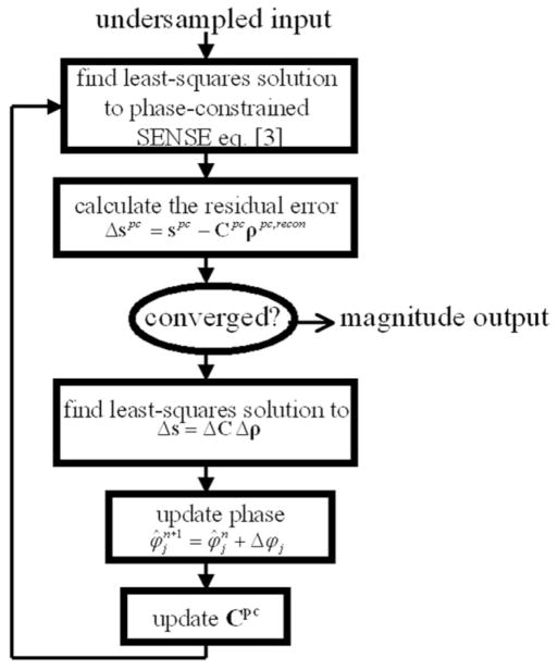
The Δφ_j are again estimated, and the process repeats itself until some convergence is reached. Figure 2 shows a flow chart detailing the steps in this reconstruction process.

FIG. 2.

The steps involved in the turboSENSE process with iterative phase refinement.

In the SENSE formalism, block diagonalization along regular Cartesian sampling schemes can be used to simplify the encoding matrix and decrease the reconstruction time (7). The reconstruction is then done entirely in the image domain. In this work, image-domain reconstructions were employed.

g-Factor

The g-factor for the phase-constrained formalism is intuitively expected to be smaller than that of SENSE since we are dealing with fewer unknowns and a matrix that is better conditioned. We analytically derive the amount of improvement in the g-factor (see Appendix). For SENSE, the g-factor is expressed as:

$$g_p=\sqrt{{({\mathbf{C}}^H{\mathbf{\Psi }}^{-1}\mathbf{C})}_p^{-1}{({\mathbf{C}}^H{\mathrm{\Psi }}^{-1}\mathbf{C})}_p}$$ [14]

The g-factor for phase-constrained SENSE is extended into a similar equation:

$$g_p^{pc}=\sqrt{{({\mathbf{C}}^{{pc}^H}{\mathbf{\Psi }}^{{pc}^{-1}}{\mathbf{C}}^{pc})}_p^{-1}{({\mathbf{C}}^H{\mathbf{\Psi }}^{-1}\mathbf{C})}_p}$$ [15]

We note the connection of the g-factor to the variance of the reconstruction in light of modeling errors. We summarize the result from the Appendix. The g-factor of phase-constrained SENSE and SENSE differ by an additive term:

$${({\mathbf{C}}^H\mathbf{C})}_p^{-1}={({\mathbf{C}}^{{pc}^H}{\mathbf{C}}^{pc})}_p^{-1}+{({((-\mathbf{M}){\mathbf{L}}^{-1})}^H{(\mathbf{L}+\mathbf{M}{\mathbf{L}}^{-1}\mathbf{M})}^{-1}(-\mathbf{M}){\mathbf{L}}^{-1})}_p$$ [16]

where L = (C^pcHC^pc)⁻¹ and M = −Im(C diag(exp(iϕ̂)))^H Re(C diag(exp(iϕ̂))) + Re(C diag(exp(iϕ̂)))^H Im(C diag(exp(iϕ̂))). The additive term can be shown to be positive semidefinite, leading to a g-factor for phase-constrained SENSE that is no larger than that of conventional SENSE.

MATERIALS AND METHODS

Simulations

Simulations were performed on a brain phantom that was scanned using an SE sequence (TE = 10 ms, TR = 200 ms, resolution = 256 × 256, flip angle = 25°) on a GE Signa CV/I 1.5T scanner with an eight-channel head coil (GE Medical Systems, Waukesha, WI, USA). Comparisons were performed among four reconstruction techniques: 1) SENSE, 2) phase-constrained SENSE, 3) turboSENSE with iterative phase refinement as described in our approach, and 4) turboSENSE with a fully resolved phase. To accomplish the latter technique, SENSE reconstruction was performed with a reduction factor of 1. The phase of the resulting reconstruction was used to approximate the ideal phase refinement, which was then fed into phase-constrained SENSE to reconstruct the data. In this fashion, we can surmise a “best-case” reconstruction with turboSENSE.

The fully sampled image was used as the reference. Undersampling was performed by removing phase-encode profiles from the full-resolution data. In this manner, comparisons will have no variability from interscan differences. To calculate the coil sensitivities, the central 48 phase encodes of each surface coil data were first apodized with a Hamming window of length 48. A global phase mismatch, such as can be expected from varying eddy currents, was then added. The coil sensitivities were then calculated by normalizing the surface coil images by the square root of the sum-of-squares. The coil sensitivities contained both the coil receiver information and the phase estimate. Measurements were taken from the image after pixels below a noise threshold were removed. The resultant image would preserve any aliasing artifact in the reconstruction. With the iterative method, we marked convergence when the residual error norm (Eq. [7]) had changed less than 1% from the previous iteration. The reduction factor refers to the amount of undersampling, and does not include the central lines used for coil sensitivity calculation.

In one simulation, reduction factors of 2, 3, 4, 5, 6, and 7 were performed. Gaussian noise at a level of 5% of the peak intensity was added to the real and imaginary channels of each coil. The g-factor was computed analytically for the image after thresholding (Eqs. [14] and [15]). Histograms of the g-factor are plotted for the various reduction factors. In addition, for the four reconstruction methods, the root-mean-squared (RMS) value of the difference between the reference and reconstructed magnitudes was also calculated. This was normalized by the mean of the reference magnitude image. The RMS is an indicator of the artifact power in the reconstructions.

In a second simulation, Gaussian noise at various levels from 1% to 13% was added to the real and imaginary channels of each coil. Reduction factors of 4 and 6 were performed. RMS differences between the reference image and each of the four reconstructed images were calculated to gauge the accuracy of the reconstructions.

In Vivo Applications

Images of human volunteers were acquired using GE Signa CV/I and TwinSpeed 1.5T scanners. The institutional review board approved the protocol, and informed consent was obtained prior to the scan. Undersampling was performed on fully sampled datasets in order to obtain comparable image quality for assessment. As in the simulations, the four reconstruction techniques were performed. In addition, SENSE with Tikhonov regularization was used as another comparison. The regularization parameter was chosen to be optimal in the L-curve sense and is based on the Twomey method proposed by Lin et al. (23,24) to trade off the dependence on the reference scan and the aliased images.

Balanced steady-state free precession (bSSFP) cine imaging data were acquired on an eight-channel cardiac phased-array coil (GE Medical Systems, Waukesha, WI, USA). The scan parameters were as follows: acquisition matrix = 256 × 224, flip angle = 20°, bandwidth = ±31.25 kHz, TR/TE = 4.5 ms/2.4 ms, FOV = 30 cm, and slice thickness = 10 mm. Ten views per segment were acquired for 20 cardiac phases, and retrospective cardiac gating was applied. The volunteers were instructed to hold their breath at inhalation to mitigate respiratory artifacts. The overall scan time took approximately 23 heartbeats. The full dataset was undersampled with a reduction factor of 5. As for the calibration, cardiac imaging has been shown to benefit from self-calibration techniques (2,22). To simulate self-calibration, the coil sensitivities were created by taking the central 32 phase encodes of the fully-sampled dataset and apodizing them through a Hamming window of length 32. In self-calibrated parallel imaging (22), the combination of apodization and a high number of central phase encodes is useful for minimizing Gibbs ringing artifacts from the central k-space profiles. The phase was estimated from the central 32 phase encodes.

Also, T₂-weighted FSE images of the brain were acquired using an eight-channel head coil. The acquisition parameters were as follows: acquisition matrix = 256 × 256, bandwidth = ±15.63 kHz, TR/TE = 5000/85 ms, flip angle = 90°, FOV = 28 cm, slice thickness = 3 mm, 18 slices, gap = 1.5 mm. The data were subsampled with a reduction factor of 7. The scan time was 2 min 45 s. A separate FSE scan was used for the calibration. It had a scan time of 45 s, 128 × 128 acquisition matrix, ±62.5 kHz bandwidth, and TR/TE = 4000/60 ms. The coil sensitivities were created by taking the central 48 phase encodes and apodizing them with a Hamming window of length 48. The phase was estimated from the central 48 phase encodes.

With the FSE images, the convergence behavior of turboSENSE with iterative phase refinement was investigated. The phase refinement process was iterated 100 times. The RMS error was calculated as function of the iteration number. The fractional change in the residual norm from the previous iteration was calculated. The accumulated time to perform the reconstruction was also tracked. Our reconstruction was implemented with Matlab software (Mathworks, Natick, MA, USA).

RESULTS

Simulations

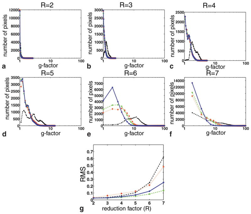
Figure 3 shows the results for the simulation with a varying reduction factor R. The g-factor histograms (Fig. 3a–f) among phase-constrained SENSE, turboSENSE with the fully-resolved phase, and turboSENSE with iterated refinement show similar bin distributions. The effects of different phase estimates do not vary substantially with the g-factor distributions. We will refer to these techniques in this discussion as magnitude-only techniques. Relative to SENSE, the g-factor histograms of the magnitude-only techniques show benefits.

FIG. 3.

a–f: g-Factor histograms for SENSE (black line), phase-constrained SENSE (red line), turboSENSE with the fully-resolved phase (green line), and turboSENSE with iterative phase refinement (blue line) for different reduction factors (R = 2–7). The latter three have similar histograms and lower g-factors than SENSE. g: RMS measurements as a function of reduction factor.

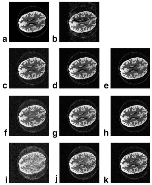
Further examination of the RMS plot (Fig. 3g) and images (Fig. 4), however, shows marginal improvement in image quality at R < 5. At R < 5, the g-factor histograms for both SENSE and the magnitude-only techniques have peaks at a g-factor value less than 2. The noise enhancement is small. At higher reduction factors, the conditioning for SENSE becomes increasingly ill conditioned, and the g-factor grows quickly. In contrast, the g-factor for the magnitude-only techniques grows but at a far lesser rate. The RMS plot (Fig. 3g) also shows that at R > 4 these differences between SENSE and turboSENSE become substantial. This can be also seen in the underlying reconstructions for these acceleration factors (Fig. 4). Of note, the phase-constrained SENSE reconstruction exhibits strong residual aliasing due to the mismatched phase. The RMS for turboSENSE with iterated refinement closely matches that of the fully-resolved phase until R > 5. TurboSENSE with the fully-resolved phase exhibits the best reconstruction of all the techniques.

FIG. 4.

Images of the phantom simulations: (a) the reference phantom, (b) a phase-constrained reconstruction at R = 4, and reconstructions for (c–e) R = 4, (f–h) 5, and (i–k) 6. c–k (left to right): SENSE, turboSENSE with iterative phase refinement, and turboSENSE with the fully-resolved phase.

The second set of simulations is shown in Fig. 5. The RMS values show increasing values as more noise is added. It is observed that because of the poorer conditioning of the SENSE reconstruction matrix at high reduction factors, SENSE reconstructions show more noise enhancement than turboSENSE reconstructions, leading to higher deviation. TurboSENSE with iterated refinement is close to turboSENSE with the fully-resolved phase at low noise levels, and it gradually deviates more at higher noise. Phase-constrained SENSE has a high RMS overall, and it is consistently higher than that of turboSENSE. Residual aliasing is a dominant factor, even when large amounts of noise are added. TurboSENSE with iterated refinement provides diminishing returns for higher noise. For R = 6, the RMS value actually surpasses phase-constrained SENSE.

FIG. 5.

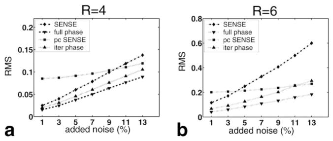
RMS measurements for SENSE, phase-constrained SENSE (“pc SENSE”), turboSENSE with the fully-resolved phase (“full phase”), and turboSENSE with iterative phase refinement (“iter phase”) as a function of the amount of added Gaussian noise. The amount of noise is the percent of the peak. Measurements were performed for (a) R = 4 and (b) R = 6.

In Vivo Applications

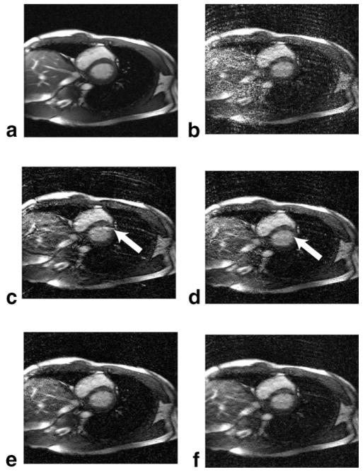
Images from one application to cine imaging are shown in Fig. 6. The SENSE reconstruction suffers from strong g-factor noise from ill-conditioned matrices. With Tikhonov regularization, the reconstruction removes much of the noise. The phase-constrained SENSE reconstruction presents strong residual aliasing, particularly of the chest wall. High fluctuations of the phase due to fat in the chest wall have caused artifacts at the left ventricular wall. The turboSENSE images do not suffer from such residual aliasing and have reduced noise amplification. TurboSENSE with iterative refinement approaches that of the fully-resolved phase. The turboSENSE images also generally have lower background noise compared to the SENSE images, an indication of higher SNR.

FIG. 6.

Comparisons of various reconstructions at R = 5: (a) fully-sampled reference image, (b) SENSE, (c) phase-constrained SENSE, (d) turboSENSE with iterative phase refinement, (e) turboSENSE with fully-resolved phase, and (f) SENSE with Tikhonov regularization. The turboSENSE images have recovered the mismatch phase of the phase-constrained reconstructions. The images from peak-systole were shown here. Ringing of the chest walls is evident due to insufficient coil-sensitivity resolution.

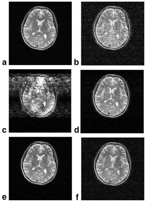
Similarly, the T₂-weighted FSE scans (Fig. 7) show a noticeable improvement with turboSENSE. The SENSE reconstruction shows more noise than turboSENSE. The reconstruction produced by phase-constrained SENSE is highly distorted by the phase mismatch. TurboSENSE recovers from this phase mismatch. It is comparable in image quality to SENSE with Tikhonov regularization. Due to the high reduction factor, residual aliasing is evident in both the regularized and turboSENSE images. The turboSENSE images have some higher edge enhancement at the cost of more salt-and-pepper noise relative to the regularized SENSE images.

FIG. 7.

Comparisons for R = 7 reconstructions of the T₂-weighted FSE images of the brain: (a) reference, (b) SENSE, (c) phase-constrained SENSE, (d) turboSENSE with iterative phase refinement, (e) turboSENSE with fully-resolved phase, and (f) SENSE with Tikhonov regularization. The phase-encoding direction is left to right.

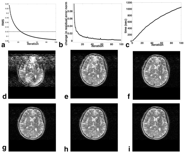
Iterative phase refinement shows no substantial change in image quality approximately around iteration number 60 (Fig. 8). The fractional change in the residual error norm and the RMS error both reflect this trend. The turboSENSE algorithm takes about 800 s (13.3 min) in total to reconstruct the image for 60 iterations. Our implementation of the SENSE algorithm takes 10 s on average. We note that our implementations are not optimized to minimize reconstruction time.

FIG. 8.

Behavior of R = 7 reconstructions of the T₂-weighted FSE images as a function of iteration number. a: RMS error. The RMS error of the SENSE reconstruction is also shown (dashed line). b: Fractional change in residual error norm from the previous iteration. c: Cumulative reconstruction time. Images are shown at iteration numbers (d) 1, (e) 20, (f) 40, (g) 60, (h) 80, and (i) 100.

DISCUSSION

The general results show that a “perfect” recovery of the spatial frequencies of the phase can lead to superior reconstructions, as is evident in the images reconstructed by turboSENSE with fully-resolved phase. Since the fully-resolved phase was obtained from a fully-sampled set, this ideal cannot be accomplished in actuality. The iterated phase-refinement approach attempts to recover the spatial frequencies from a limited dataset.

Iterative refinement in turboSENSE reduces aliasing at the possible cost of noise amplification. The in vivo images show that residual aliasing due to phase at high spatial frequencies has been removed to a large extent. However, the iterative nature of the phase refinement uses the acquired noisy dataset to improve the phase and consequently adds noise during the process of updating the phase to the coil sensitivity matrix. The noise simulations (Fig. 5) show a relatively constant difference between turboSENSE with iterative phase refinement and the fully-resolved phase at up to 9% of added noise. Above 9%, the difference grows as the effectiveness of the iterative refinement diminishes. In addition, at higher reduction factors, the conditioning of the phase refinement matrix, ΔC (Eq. [12]), will also affect the accuracy of the phase refinement. Our approach may lose some of the SNR relative to conventional phase-constrained SENSE, as is evident in the in vivo images. The iterative technique may be considered a compromise between the strong residual artifacts of phase-constrained SENSE and the high noise enhancement of conventional SENSE. Suppressing residual artifacts may be paramount at the cost of some SNR with respect to a particular patient, where, for example in Fig. 6, accurate delineation of the left ventricle is important for measurement of wall thickness. It would be also useful for detecting lesions on the edge of visibility, where it is critical to eliminate artifacts and suppress large amounts of noise.

TurboSENSE with iterative phase-refinement reconstruction offers a significant improvement over SENSE when reduction factors approach the theoretical limit. With the eight-channel coil systems used throughout the course of this investigation, reduction factors greater than 4 showed an improvement in g-factor noise mitigation. At lower reduction factors, the difference between SENSE and the new reconstruction approach was harder to distinguish visually, although both theory and measurements documented SNR benefits. It is suspected that the symmetrical layout of the coils allows for relatively good conditioning of the coil sensitivity matrix. The low g-factor values at reduction factors of 2, 3, and 4 reaffirm this belief. The depth sensitivity from the lateral coils is not high enough to produce good sensitivity at factors higher than 4. Finally, the in vivo examples exhibited image quality comparable to that of the phantom images with higher reduction factors, in spite of the more realistic coil sensitivities with noisy estimates.

The diminished impact of phase-constrained SENSE and its turboSENSE offshoot at lower reduction factors may also be fundamentally limited by the use of the image phase to improve the reconstruction. The general smoothness of the image phase correlates the real and imaginary components of the coil sensitivities. The conditioning of the unfolding matrix for phase-constrained SENSE relative to conventional SENSE at low reduction factors is improved only a little.

It is important to note that the g-factor alone is insufficient to determine the quality of the image reconstruction. The integration of phase into the decoding matrix does not appear to significantly alter the g-factor among phase-constrained SENSE, turboSENSE with iterated refinement, and turboSENSE with the fully-resolved phase, as shown in the histograms, but it substantially affects image quality. Specifically, phase-constrained SENSE also has lower g-factors than SENSE, but it is clearly limited by the errors in the phase estimate, leading to inaccurate rather than imprecise image reconstructions. The simulations furthermore show that a phase offset added to the coil sensitivities can cause strong residual aliasing in conventional phase-constrained SENSE. Investigating the RMS, difference, or other similar scheme will complement and support g-factor calculations. Equation [5] serves as a method to measure the effects of both noise and modeling errors on the SENSE reconstruction.

TurboSENSE with iterative phase refinement exhibits slow convergence behavior, especially with high reduction factors. Performing two matrix inversions per phase update is costly. Our implementation requires about an 80-fold increase over a SENSE reconstruction. The convergence of turboSENSE would benefit from methods such as improving the initial estimate or adaptively changing the rate of the phase update.

It was previously shown (15,16) that phase-constrained SENSE techniques can be applied with partial-Fourier sampling schemes. The theory of the iterative phase-refinement technique was developed in k-space and conceivably can be extended to these sampling schemes. As shown with our simulations, turboSENSE can use a phase estimate that was estimated at a lower resolution, which makes it compatible with partial-Fourier schemes. In addition, imperfect phase estimates in partial-Fourier techniques have been known to contribute to ringing in the reconstruction. Iterative phase refinement may help recover some of this phase mismatch and diminish the ringing, although this would require further investigation. Applying iterative phase refinement from the k-space domain would, however, considerably lengthen the reconstruction time.

CONCLUSIONS

TurboSENSE with iterative phase refinement provides a new way to approach the phase-constrained SENSE problem. The greatest benefits occur at high reduction factors where the SENSE matrix is extremely ill conditioned. TurboSENSE can be considered a trade-off of the SENSE and phase-constrained SENSE techniques. The iterative technique offers SNR improvement over SENSE while reducing residual aliasing compared to phase-constrained SENSE.

APPENDIX

To relate the g-factor of phase-constrained SENSE and SENSE, we reformulate the SENSE matrix in a form similar to the phase-constrained SENSE formulation. We examine the effects on the g-factor along the way.

Consider the SENSE matrix C with reduction factor r. Let the g-factor be $g_p^c$ and p ∈ {1, …,r}. Let c be the diagonal of the covariance coil sensitivity matrix (C^HC)⁼¹,

$${\mathbf{c}}_p={({\mathbf{C}}^H\mathbf{C})}_p^{-1}$$ [A1]

By definition, $g_p^C=\sqrt{{\mathbf{c}}_p{({\mathbf{C}}^H\mathbf{C})}_p}$.

SENSE can be reexpressed into real and imaginary parts with no loss of generality:

$$\mathbf{D}=\left[\begin{array}{cc}Re(\mathbf{C})& -Im(\mathbf{C})\\ Im(\mathbf{C})& Re(\mathbf{C})\end{array}\right]$$ [A2]

The g-factor for D remains the same for both the real and imaginary components of the magnetization, and p ∈ {1, …,2r}. In other words,

$$g_p^D=\{\begin{array}{cc}{g}_p^C,& 1\le p\le r\\ g_{p-r}^C,& r<p\le 2r\end{array}$$ [A3]

We will use this result later in the Appendix.

Now, we consider the case in which we right-multiply the SENSE matrix by the phase estimate. Let B = CF, where F is an invertible orthogonal diagonal matrix. F can represent the phase estimate, diag(exp(iϕ̂)), for example. We derive the g-factor, $g_p^B$, by examining the diagonal of the covariance coil sensitivity matrix of B:

$$\begin{array}{c}{({\mathbf{B}}^H\mathbf{B})}_p^{-1}={({(\mathbf{CF})}^H(\mathbf{CF}))}_p^{-1}={({\mathbf{F}}^H({\mathbf{C}}^H\mathbf{C})\mathbf{F})}_p^{-1}\\ ={({\mathbf{F}}^{-1}{({\mathbf{C}}^H\mathbf{C})}^{-1}\mathbf{F})}_p,\text{since}\mathbf{F}\text{is}\text{invertible}\text{and}\text{orthogonal}\\ ={({\mathbf{C}}^H\mathbf{C})}_p^{-1},\text{since}\mathbf{F}\text{is}\text{diagonal}\\ ={\mathbf{c}}_p,\text{by}[\text{A}1]\end{array}$$ [A4]

Therefore, the diagonals are the same, and consequently, $g_p^B=g_p^C$. So far, as we would expect, the reformulation does not change the noise amplification.

We add that splitting B into its real and imaginary components will not change the g-factor. This is analogous to the result from Eq. [A2]. Specifically, we define a matrix U:

$$\mathbf{U}=\left[\begin{array}{cc}Re(\mathbf{B})& -Im(\mathbf{B})\\ Im(\mathbf{B})& Re(\mathbf{B})\end{array}\right]$$ [A5]

and we have the g-factor of U, $g_p^U=g_p^D$. From this result, right-multiplying the SENSE matrix by the phase estimate and subsequently splitting the matrix into real and imaginary components do not change the noise amplification.

Using the above results, we can finally relate the g-factor of phase-constrained SENSE to SENSE. We approach this by deriving the relationship between the diagonal of the covariance coil sensitivity matrix of phase-constrained SENSE to that of SENSE. Let

$${\mathbf{C}}^{pc}=\left[\begin{array}{c}Re(\mathbf{B})\\ Im(\mathbf{B})\end{array}\right]$$ [A6]

Let v be the diagonal of the phase-constrained SENSE matrix:

$${\mathbf{v}}_p={({\mathbf{C}}^{{pc}^H}{\mathbf{C}}^{pc})}_p^{-1},p\in \{1,\dots ,r\}$$ [A7]

$$={(Re{(\mathbf{B})}^{H}Re(\mathbf{B})+Im{(\mathbf{B})}^{H}Im(\mathbf{B}))}_p^{-1}={\mathbf{L}}_p^{-1}$$ [A8]

where L = (Re(B)^HRe(B) + Im(B)^HIm(B)) for convenience.

On the other hand, for SENSE,

$${\mathbf{u}}_p={({\mathbf{U}}^H\mathbf{U})}_p^{-1},p\in \{1,\dots ,2r\}={\left[\begin{array}{cc}Re{(\mathbf{B})}^{H}Re(\mathbf{B})+Im{(\mathbf{B})}^{H}Im(\mathbf{B})& Im{(\mathbf{B})}^{H}Re(\mathbf{B})-Re{(\mathbf{B})}^{H}Im(\mathbf{B})\\ -Im{(\mathbf{B})}^{H}Re(\mathbf{B})+Re{(\mathbf{B})}^{H}Im(\mathbf{B})& Re{(\mathbf{B})}^{H}Re(\mathbf{B})+Im{(\mathbf{B})}^{H}Im(\mathbf{B})\end{array}\right]}_{\text{p}}^{-1}={\left[\begin{array}{cc}\mathbf{L}& -\mathbf{M}\\ \mathbf{M}& \mathbf{L}\end{array}\right]}_p^{-1}$$ [A9]

where M = −Im(B)^HRe(B) + Re(B)^HIm(B). We observe that M is skew-symmetric. The inverse of Eq. [A9] can be rewritten by its Schur decomposition (25):

$$\begin{array}{c}{\mathbf{u}}_p={\left(\left[\begin{array}{cc}\mathbf{I}& \mathbf{0}\\ -{\mathbf{L}}^{-\mathbf{1}}\mathbf{M}& \mathbf{I}\end{array}\right]\left[\begin{array}{cc}{(\mathbf{L}+\mathbf{M}{\mathbf{L}}^{-\mathbf{1}}\mathbf{M})}^{-\mathbf{1}}& \mathbf{0}\\ \mathbf{0}& {\mathbf{L}}^{-\mathbf{1}}\end{array}\right]\left[\begin{array}{cc}\mathbf{I}& \mathbf{M}{\mathbf{L}}^{-\mathbf{1}}\\ \mathbf{0}& \mathbf{I}\end{array}\right]\right)}_p\\ ={\left[\begin{array}{ll}{(\mathbf{L}+\mathbf{M}{\mathbf{L}}^{-\mathbf{1}}\mathbf{M})}^{-1}\hfill & {(\mathbf{L}+\mathbf{M}{\mathbf{L}}^{-\mathbf{1}}\mathbf{M})}^{-\mathbf{1}}\mathbf{M}{\mathbf{L}}^{-\mathbf{1}}\hfill \\ -{\mathbf{L}}^{-\mathbf{1}}\mathbf{M}{(\mathbf{L}+\mathbf{M}{\mathbf{L}}^{-\mathbf{1}}\mathbf{M})}^{-\mathbf{1}}\hfill & {\mathbf{L}}^{-\mathbf{1}}+{((-\mathbf{M}){\mathbf{L}}^{-\mathbf{1}})}^H{(\mathbf{L}+\mathbf{M}{\mathbf{L}}^{-\mathbf{1}}\mathbf{M})}^{-\mathbf{1}}(-\mathbf{M}){\mathbf{L}}^{-\mathbf{1}}\hfill \end{array}\right]}_p\end{array}$$ [A10a]

where (L + ML⁻¹M)⁻¹ is the Schur complement. u can also alternatively be decomposed as:

$$\begin{array}{c}{\mathbf{u}}_p={\left(\left[\begin{array}{cc}\mathbf{I}& {\mathbf{L}}^{-\mathbf{1}}\mathbf{M}\\ \mathbf{0}& \mathbf{I}\end{array}\right]\left[\begin{array}{cc}\mathbf{L}& \mathbf{0}\\ \mathbf{0}& {(\mathbf{L}+\mathbf{M}{\mathbf{L}}^{-\mathbf{1}}\mathbf{M})}^{-\mathbf{1}}\end{array}\right]\left[\begin{array}{cc}\mathbf{I}& \mathbf{0}\\ -\mathbf{M}{\mathbf{L}}^{-\mathbf{1}}& \mathbf{I}\end{array}\right]\right)}_p\\ ={\left[\begin{array}{cc}{\mathbf{L}}^{-\mathbf{1}}+{((-\mathbf{M}){\mathbf{L}}^{-\mathbf{1}})}^H{(\mathbf{L}+\mathbf{M}{\mathbf{L}}^{-\mathbf{1}}\mathbf{M})}^{-1}(-\mathbf{M}){\mathbf{L}}^{-\mathbf{1}}& {\mathbf{L}}^{-\mathbf{1}}\mathbf{M}{(\mathbf{L}+\mathbf{M}{\mathbf{L}}^{-\mathbf{1}}\mathbf{M})}^{-\mathbf{1}}\\ -{(\mathbf{L}+\mathbf{M}{\mathbf{L}}^{-\mathbf{1}}\mathbf{M})}^{-\mathbf{1}}\mathbf{M}{\mathbf{L}}^{-\mathbf{1}}& {(\mathbf{L}+\mathbf{M}{\mathbf{L}}^{-\mathbf{1}}\mathbf{M})}^{-\mathbf{1}}\end{array}\right]}_p\end{array}$$ [A10b]

$$={\left[\begin{array}{ll}{\mathbf{L}}^{-\mathbf{1}}+{((-\mathbf{M}){\mathbf{L}}^{-\mathbf{1}})}^H{(\mathbf{L}+\mathbf{M}{\mathbf{L}}^{-\mathbf{1}}\mathbf{M})}^{-1}(-\mathbf{M}){\mathbf{L}}^{-\mathbf{1}}\hfill & {\mathbf{L}}^{-\mathbf{1}}\mathbf{M}{(\mathbf{L}+\mathbf{M}{\mathbf{L}}^{-\mathbf{1}}\mathbf{M})}^{-\mathbf{1}}\hfill \\ -{(\mathbf{L}+\mathbf{M}{\mathbf{L}}^{-\mathbf{1}}\mathbf{M})}^{-\mathbf{1}}\mathbf{M}{\mathbf{L}}^{-\mathbf{1}}\hfill & {\mathbf{L}}^{-\mathbf{1}}+{((-\mathbf{M}){\mathbf{L}}^{-\mathbf{1}})}^H{(\mathbf{L}+\mathbf{M}{\mathbf{L}}^{-\mathbf{1}}\mathbf{M})}^{-\mathbf{1}}(-\mathbf{M}){\mathbf{L}}^{-\mathbf{1}}\hfill \end{array}\right]}_p,$$ [A11]

by inspecting the elements of [A10a] and [A10b].

To relate phase-constrained SENSE and SENSE, we compare the block matrices on the diagonals of v and u, which are L⁻¹ and L⁻¹ + ((−M)L⁻¹)^H(L + ML⁻¹M)⁻¹ (−M)L⁻¹, respectively. By inspection, the difference between u and v is the term:

$${((-\mathbf{M}){\mathbf{L}}^{-1})}^H{(\mathbf{L}+\mathbf{M}{\mathbf{L}}^{-\mathbf{1}}\mathbf{M})}^{-1}(-\mathbf{M}){\mathbf{L}}^{-\mathbf{1}}$$ [A12]

We now observe that, by Eq. [A9], u_p is positive semidefinite. A property of positive semidefinite matrices is that the diagonal elements are nonnegative. The Schur complement is also positive semidefinite. Equation [A12] is positive semidefinite and its diagonal elements are guaranteed to be nonnegative. Thus, the g-factor of SENSE is no smaller than that of phase-constrained SENSE.

We can now relate the g-factor of SENSE to the g-factor of phase-constrained SENSE:

$$\begin{array}{l}{\mathbf{u}}_p={({\mathbf{U}}^H\mathbf{U})}_p^{-1}={({\mathbf{D}}^H\mathbf{D})}_p^{-1},\text{by}[\text{A}5]\\ ={({\mathbf{C}}^H\mathbf{C})}_p^{-1},\text{for}p\in \{1,\dots ,r\},\text{by}[\text{A}3]\end{array}$$ [A13a]

Also,

$$\begin{array}{l}{\mathbf{u}}_p={\mathbf{L}}_p^{-1}+{({((-\mathbf{M}){\mathbf{L}}^{-\mathbf{1}})}^H{(\mathbf{L}+\mathbf{M}{\mathbf{L}}^{-1}\mathbf{M})}^{-1}(-\mathbf{M}){\mathbf{L}}^{-\mathbf{1}})}_p,\text{by}[\text{A}10],[\text{A}11]\\ ={({\mathbf{C}}^{{pc}^H}{\mathbf{C}}^{pc})}_p^{-1}+{(((-\mathbf{M}){\mathbf{L}}^{-\mathbf{1}})H{(\mathbf{L}+\mathbf{M}{\mathbf{L}}^{-1}\mathbf{M})}^{-1}(-\mathbf{M}){\mathbf{L}}^{-\mathbf{1}})}_{\mathbf{p}},\text{by}[\text{A}8]),\end{array}$$ [A13b]

Thus we have a relationship for the covariance coil-sensitivity matrix, and consequently the g-factor between phase-constrained SENSE (Eq. [A13b]) and SENSE (Eq. [A13a]).

References

- 1.Thunberg P, Karlsson M, Wigstrom L. Accuracy and reproducibility in phase contrast imaging using SENSE. Magn Reson Med. 2003;50:1061–1068. doi: 10.1002/mrm.10634. [DOI] [PubMed] [Google Scholar]
- 2.Kellman P, Epstein F, McVeigh ER. Adaptive sensitivity encoding incorporating temporal filtering (TSENSE) Magn Reson Med. 2001;45:846– 852. doi: 10.1002/mrm.1113. [DOI] [PubMed] [Google Scholar]
- 3.Yoshioka H, Takahashi N, Yamaguchi M, Lou D, Saida Y, Itai Y. Double arterial phase dynamic MRI with sensitivity encoding (SENSE) for hypervascular hepatocellular carcinomas. J Magn Reson Imaging. 2002;16:259–266. doi: 10.1002/jmri.10146. [DOI] [PubMed] [Google Scholar]
- 4.Bammer R, Keeling SL, Augustin M, Pruessmann KP, Wolf R, Stollberger R, Hartung HP, Fazekas F. Improved diffusion-weighted single-shot EPI in stroke using sensitivity encoding. Magn Reson Med. 2001;46:548–554. doi: 10.1002/mrm.1226. [DOI] [PubMed] [Google Scholar]
- 5.Bammer R, Auer M, Keeling SL, Augustin M, Stables LA, Prokesch RW, Stollberger R, Moseley ME, Fazekas F. Diffusion tensor imaging using single-shot SENSE-EPI. Magn Reson Med. 2002;48:128–136. doi: 10.1002/mrm.10184. [DOI] [PubMed] [Google Scholar]
- 6.Pelc NJ, Herfkens RJ, Shimakawa A, Enzmann DR. Phase contrast cine magnetic resonance imaging. Magn Reson Q. 1991;7:229–254. [PubMed] [Google Scholar]
- 7.Pruessman KP, Weiger M, Scheidegger MB, Boesiger P. SENSE: sensitivity encoding for fast MRI. Magn Reson Med. 1999;42:952–962. [PubMed] [Google Scholar]
- 8.Noll DC, Nishimura GD, Macovski A. Homodyne detection in magnetic resonance imaging. IEEE Trans Med Imaging. 1991;10:154–163. doi: 10.1109/42.79473. [DOI] [PubMed] [Google Scholar]
- 9.Cuppen JM. U.S. Patent 4,853,635. Method of reconstructing a nuclear magnetization distribution from a partial magnetic resonance measurement. 1989
- 10.McGibney G, Smith MR, Nichols ST, Crawley A. Quantitative evaluation of several partial Fourier reconstruction algorithms used in MRI. Magn Reson Med. 1993;30:51–59. doi: 10.1002/mrm.1910300109. [DOI] [PubMed] [Google Scholar]
- 11.Haacke EM, Lindskogj ED, Lin W. A fast, iterative, partial-Fourier technique capable of local phase recovery. J Magn Reson. 1991;92:126–145. [Google Scholar]
- 12.Clayton DB, Bammer R. Methods for SENSE reconstruction with partial k-space acquisition. Proceedings of the 13th Annual Meeting of ISMRM; Miami Beach, FL, USA. 2005. p. Abstract 686. [Google Scholar]
- 13.Samsonov AA, Kholmovski EG, Parker DL, Johnson CR. POCSENSE: POCS-based reconstruction for sensitivity encoded magnetic resonance imaging. Magn Reson Med. 2004;52:1397–1406. doi: 10.1002/mrm.20285. [DOI] [PubMed] [Google Scholar]
- 14.Samsonov AA, Kholmovski EG. Method for quality improvement of images reconstructed from sensitivity encoded data. Proceedings of the 10th Annual Meeting of ISMRM; Honolulu, HI, USA. 2002. p. Abstract 2408. [Google Scholar]
- 15.Willig-Onwuachi JD, Yeh EN, Grant AK, Ohliger MA, McKenzie CA, Sodickson DK. Phase-constrained parallel MR image reconstruction. J Magn Reson. 2005;176:187–198. doi: 10.1016/j.jmr.2005.06.004. [DOI] [PubMed] [Google Scholar]
- 16.Bydder M, Robson MD. Partial Fourier partially parallel imaging. Magn Reson Med. 2005;53:1393–1401. doi: 10.1002/mrm.20492. [DOI] [PubMed] [Google Scholar]
- 17.Samsonov AA, Bydder M. Adaptive phase-constrained reconstruction for partial Fourier partially parallel imaging. Proceedings of the 13th Annual Meeting of ISMRM; Miami Beach, FL, USA. 2005. p. Abstract 2454. [Google Scholar]
- 18.Lew C, Spielman D, Bammer R. TurboSENSE: phase estimation in temporal phase-constrained phase imaging. Proceedings of the 12th Annual Meeting of ISMRM; Kyoto, Japan. 2004. p. Abstract 2646. [Google Scholar]
- 19.Lew C, Spielman D, Chan F, Bammer R. Improved TurboSENSE with iterated conjugate gradient phase refinement. Proceedings of the 13th Annual Meeting of ISMRM; Miami Beach, FL, USA. 2005. p. Abstract 2443. [Google Scholar]
- 20.Reeder SB, Wen Z, Yu H, Pineda AR, Gold GE, Markl M, Pelc NJ. Multicoil Dixon chemical species separation with iterative least-squares estimation method. Magn Reson Med. 2004;51:35–45. doi: 10.1002/mrm.10675. [DOI] [PubMed] [Google Scholar]
- 21.Kay SM. Fundamentals of statistical signal processing: estimation theory. Saddle River, NJ: Prentice-Hall, Inc; 1993. [Google Scholar]
- 22.McKenzie CA, Yeh EN, Ohliger MA, Price MD, Sodickson DK. Self-calibrating parallel imaging with automatic coil sensitivity extraction. Magn Reson Med. 2002;47:529–538. doi: 10.1002/mrm.10087. [DOI] [PubMed] [Google Scholar]
- 23.Lin FH, Kwong KK, Belliveau JW, Wald LL. Parallel imaging reconstruction using automatic regularization. Magn Reson Med. 2004;51:559–567. doi: 10.1002/mrm.10718. [DOI] [PubMed] [Google Scholar]
- 24.Twomey S. On the numerical solution of Fredholm integral equations of the first kind by the inversion of the linear system produced by quadrature. J Assoc Comput Mach. 1963;10:97–101. [Google Scholar]
- 25.Golub G, Van Loan C. Matrix computations. Baltimore: John Hopkins University; 1996. [Google Scholar]