Comparison of hemodynamics of intracranial aneurysms between MR fluid dynamics using 3D cine phase-contrast MRI and MR-based computational fluid dynamics

Abstract

Introduction

Hemodynamics is thought to play a very important role in the initiation, growth, and rupture of intracranial aneurysms. The purpose of our study was to compare hemodynamics of intracranial aneurysms of MR fluid dynamics (MRFD) using 3D cine PC MR imaging (4D-Flow) at 1.5 T and MR-based computational fluid dynamics (CFD).

Methods

4D-Flow was performed for five intracranial aneurysms by a 1.5 T MR scanner. 3D TOF MR angiography was performed for geometric information. The blood flow in the aneurysms was modeled using CFD simulation based on the finite element method. We used MR angiographic data as the vascular models and MR flow information as boundary conditions in CFD. 3D velocity vector fields, 3D streamlines, shearing velocity maps, wall shear stress (WSS) distribution maps and oscillatory shear index (OSI) distribution maps were obtained by MRFD and CFD and were compared.

Results

There was a moderate to high degree of correlation in 3D velocity vector fields and a low to moderate degree of correlation in WSS of aneurysms between MRFD and CFD using regression analysis. The patterns of 3D streamlines were similar between MRFD and CFD. The small and rotating shearing velocities and higher OSI were observed at the top of the spiral flow in the aneurysms. The pattern and location of shearing velocity in MRFD and CFD were similar. The location of high oscillatory shear index obtained by MRFD was near to that obtained by CFD.

Conclusion

MRFD and CFD of intracranial aneurysms correlated fairly well.

Introduction

Hemodynamics is thought to play a very important role in the initiation, growth, and rupture of intracranial aneurysms. Therefore, accurate hemodynamic information would be very useful for understanding pathogenesis of aneurysms. To obtain hemodynamic information, we need time-resolved three-dimensional (3D) and three-directional flow velocity data set (3D velocity vector fields) of the vascular structure. We can generate 3D streamlines, 3D particle traces, or 3D pathlines using information of 3D velocity vector fields to visualize the blood flow [1]. Wall shear stress (WSS) and oscillatory shear index (OSI) are important biological parameters affecting the vascular wall [2, 3]. WSS is a dynamic frictional force induced by a viscous fluid moving across a surface of solid material and is defined as the multiplication of fluid viscosity and shearing velocity of the neighboring vascular wall. OSI shows the degree of the fluctuation of the WSS during cardiac cycle. WSS and OSI can be calculated using flow velocities near the wall.

Three main methods are used to obtain the data set of the 3D velocity vector fields, which are as follows: (1) experimental fluid dynamics or in vitro fluid dynamics including laser Doppler velocimetry (LDV) [4] and particle image velocimetry [5]; (2) in vivo fluid dynamics including cine phase-contrast (PC) MR imaging [6–9] and Doppler ultrasound; and (3) computational fluid dynamics (CFD) or in silico fluid dynamics [10–20]. This study focused on in vivo fluid dynamics using 3D cine PC MR imaging and CFD.

CFD is a computer simulation based on many assumptions that requires vascular morphological information, boundary conditions (i.e., temporal flow information of the inlet and outlet surfaces), and initial conditions. CFD for intracranial aneurysms has been performed recently [10–20]. If we use accurate vascular models and accurate boundary conditions, CFD can provide us with precise 3D velocity vector fields with high spatial resolution and high temporal resolution. On the contrary, 3D cine phase-contrast MR imaging (time-resolved three-dimensional phase-contrast MRI, 4D-Flow) can measure blood flow velocities (i.e., 3D velocity vector fields) in the vessels in living human beings [6–9], although its spatial resolution and temporal resolution are somewhat lower than those of CFD. There have been few papers comparing the hemody-namics of intracranial aneurysms between MR fluid dynamics (MRFD) using 4D-Flow and MR-based CFD.

The purpose of our study was to compare MRFD using 4D-Flow and CFD based on 3D velocity vector fields, 3D streamlines, shearing velocity, WSS, and OSI of intracranial aneurysms. In this study, we used MR angiographic data for the vascular models and MR flow information for the boundary conditions in CFD.

Materials and methods

Subjects

This study was approved by the institutional review board of our university. Five patients (two male, three female, 51 to 71 years old, 62.8 years old on average) had the following five unruptured aneurysms (their diameters ranged from 3 to 8 mm, 5.7 mm on average); one basilar artery-superior cerebellar artery (BA-SCA) aneurysm, two internal carotid-posterior communicating (IC-PC) artery aneurysms, one middle cerebral artery (MCA) bifurcation aneurysm, and one internal carotid-ophthalmic (IC-Oph) artery aneurysm. Informed consent was obtained from all patients.

MR imaging

MR imaging was performed by a 1.5T MR scanner (Signa Infinity Twinspeed with Excite (version 12), GE Healthcare, Milwaukee, WI, USA) with a commercially available eight-channel head array coil. 4D-Flow provides us with time-resolved 3D voxel data, each of which has three-directional flow velocity components [6]. Imaging parameters for 4D-Flow were as follows: repetition time (TR)/echo time (TE)/number of excitation (NEX), 5.8/2.1/1; flip angle (FA), 15; field of view (FOV), 160×160×32 mm; matrix, 160×160× 20; voxel size, 1×1×1.6 mm; reconstructed matrix with the aid of zero filled interpolation processing (ZIP), 160×160× 40; reconstructed voxel size with the aid of ZIP, 1×1× 0.8 mm; velocity encoding, 60–100 cm/s; band width (BW), 62.5 kH; slew rate, 77 mT/m/ms; imaging time, 15 to 25 min; transaxial direction; and retrospective gating with ECG, 20 phases. Row data of 4D-Flow was transferred to a personal computer (Intel Pentium4 CPU, 3.2 GHz, 2,048 MB RAM, Linux). 4D-Flow imaging provided five kinds of images, i.e., magnitude images, x-, y-, z-encoded PC MR images and speed images. Therefore, a total of 2,000 images were reconstructed in about 170 min. Details are described elsewhere [6].

3D time-of-flight (TOF) MR angiography was performed for geometric information. Imaging parameters for 3D TOF MR angiography were as follows: TR/TE/NEX, 40/2.2/1; FA, 30; FOV, 160×160×32 mm; matrix, 160× 160×20; reconstructed matrix with the aid of ZIP, 160× 160×40; voxel size, 1×1×1.6 mm; reconstructed voxel size with the aid of ZIP, 1×1×0.8 mm; BW, 32 kH; imaging time, 2 min 40 s; and transaxial direction.

MR fluid dynamics

4D-Flow data set and MR angiographic data set mentioned in the above section were transferred to a personal computer (Intel Pentium4 CPU, 3.2 GHz, 2,048 MB RAM, Microsoft Windows XP) in DICOM format. We decided region of interest including the aneurysm and the parent arteries from the 4D-Flow and MR angiographic data set. Segmentation was performed for vascular wall structures from 3D data sets of MR angiography or one proper phase of magnitude images of 4D-Flow with the aid of region growing method [21]. At the beginning of the segmentation of vessel by region growing method, we chose one point inside the vessel, another point outside of the vessel, and the parameter, determining whether points were inside or outside of the vessel. Regions inside or outside of the vessel grew from each reference point until the whole vascular structure was segmented. Vascular shapes were then created by marching cubes method [22]. We changed the reference points and the parameter for segmentation until the final vascular shape matched the edge of the vascular shape on the original MR angiographic images or magnitude images of 4D-Flow.

3D and three-directional flow information was interpolated with the spatial resolution of 0.5×0.5×0.5 mm using the 3D data sets obtained by 4D-Flow. We visualized 3D velocity vector fields based on the flow information included in 4D-Flow data. We set several planes traversing the aneurysm and the parent arteries and generated 3D streamlines with the use of Runge–Kutta method [1]. 3D streamlines are integrated traces along instantaneous velocity vector field, color coded according to the local velocity magnitude.

WSS is a dynamic frictional force induced by a viscous fluid moving across a surface of solid material [2]. Shearing velocity is calculated by dividing velocity along the wall by distance from wall to the velocity measuring point. WSS is defined as the multiplication of fluid viscosity and shearing velocity of the neighboring vascular wall [2]. We chose one WSS calculation point (S₀) and three reference points (S₁ to S₃) at regular interval d of the normal to the wall (Fig. 1). S₀ was located at the wall and S₁ to S₃ were located in the vascular structure. Velocity vectors at S₁, S₂, and S₃ were linearly interpolated by the surrounding data points with the use of linear interpolation method. The slope of the curve (derivative value) of the velocity vector profile at S₀ was the velocity vector gradient at S₀. We set the velocity at S₀ to zero, and the velocity vector gradient at the wall was estimated with Lagrange’s polynomial interpolation formula. WSS vector at S₀ was calculated by multiplying viscosity by the tangential velocity vector gradient perpendicular to the normal to the wall (i.e., tangential shearing velocity vector). WSS was the strength of the WSS vector. We used a blood viscosity of 0.0038 Pas for the calculation. Our method was similar to those reported by Masaryk [23] and Cheng [24], with the main difference being that our method was three-dimensional not two-dimensional. In this method the probability that the WSS calculation point (S₀) and the three reference points (S₁ to S₃) were located in different and neighboring voxels was as high as possible. The distance necessary to maximize probability that S₀ to S₃ occupied neighboring voxels was determined by numerical experiment for each model and was set as approximately 1.15 times voxel spacing, 0.575 mm in this study. We calculated shearing velocity and WSS and obtained contour maps of these.

Fig. 1.

Calculation method of wall shear stress (WSS). For one arbitrary calculation point (S₀) on the wall surface, we choose three reference points (S₁ to S₃) of the normal to the wall inside of the lumen at regular interval d. Velocity vectors at S₁, S₂, and S₃ are interpolated by surrounding data points with the use of linear interpolation method. The slope of velocity profile (derivative value=f′ (S₀)) of S₀ is the velocity vector gradient at S₀. We set the velocity at S₀ to zero and the velocity vector gradient at the wall is estimated with Lagrange’s polynomial interpolation formula. WSS vector at S₀ is calculated by multiplying viscosity by the tangential velocity vector gradient perpendicular to the normal to the wall (i.e., tangential shearing velocity vector). WSS is the strength of the WSS vector. f′(S₀), velocity vector gradient at the wall

Because endothelial cells are reported to be very sensitive to the instantaneous fluctuation of WSS [3], we calculated OSI based on the WSS vector. OSI was defined as $\text{OSI}=\frac{1}{2}\left(1-\frac{\left|\underset{0}{\overset{\tau }{\int }}\mathit{wssidt}\right|}{\underset{0}{\overset{\tau }{\int }}\mid \mathit{wssi}\mid dt}\right)$ where WSS_i was instantaneous WSS vectors [3]. OSI ranged from 0 to 0.5 and larger OSI meant that instantaneous WSS vector fluctuated more from the main stream direction at the calculated point during one cardiac cycle.

Segmentation and creation of vascular model, calculation of 3D streamlines, shearing velocity, WSS, and OSI mentioned previously were done in about 1 h by our in-house software, which was written by one of the authors (Y.O.) in Visual C++ language.

Computational Fluid Dynamics

We created a tetrahedral mesh in each aneurysm model, the same model used for MRFD, with a fine mesh near the wall for more accurate calculation of flow velocities around the wall using commercially available software (Amira, Mercury Computer Systems, Inc., USA). The size of the mesh increased away from the wall. The minimum, maximum, and average length of the nodes were 0.009, 0.777, and 0.220 mm, respectively. The total number of meshes ranged from 237,687 to 753,178.

CFD was performed for the models with the use of a finite element solver (Acusolve, ACUSIM Software, Inc., USA) under the governing equations of mass conservation and Navie–Stokes, and 3D velocity vector fields were obtained for the models. We assumed the circulating fluid as Newtonian and incompressible with a specific density of 1.054 kg/m³ and viscosity of 0.0038 Pas. A rigid wall with no-slip conditions was applied. The flow measurement using 4D-Flow data demonstrated that the timing of peak velocity of the inflow and outflow of the parent arteries of the aneurysms was the same for all aneurysms. Thus, these aneurysms were thought not to significantly change their volume during cardiac cycle and so, CFD using rigid vascular model might be acceptable to simulate hemodynamics of the aneurysms.

Temporal flow vectors for each point on the inlet surface, which were linearly interpolated based on the 4D-Flow data, were used as boundary conditions for CFD. A traction-free boundary condition was applied to the outlets for the BA-SCA aneurysm with three outlets, one IC-PC artery aneurysm with one outlet and the IC-Oph artery aneurysm with one outlet. We set the flow volume ratio of the outlets based on the 4D-Flow data set for the MCA bifurcation aneurysm with two outlets and another IC-PC artery aneurysm with two outlets.

Three cardiac cycles were calculated with 90 or 180 steps per one cardiac cycle, and the result of CFD was based on the third cycle. The calculation time for CFD was from 10 to 15 h using the CPU with 2.5 GHz.

We visualized 3D velocity vector fields and calculated 3D streamlines, shearing velocities, WSS, and OIS using the same method used for MRFD. In calculating WSS, the regular interval of three reference points was set at 0.575 mm.

We also obtained WSS based on the shearing velocities calculated from the flow velocities of nodes located at the outermost layer of the vasculature. The shearing velocities were calculated by dividing tangential velocities, perpendicular to the normal to the wall of nodes located at the outermost layer of the wall by distance of nodes from the wall (0.009 mm).

Evaluation

We correlated the 3D velocity vector fields and WSS of MRFD with those of MR-based CFD using a regression analysis for all five aneurysms. Analyses were made for corresponding intravascular data points for 3D velocity vector fields and for corresponding surface points for WSS. We analyzed both aneurysms and parent arteries. As MRFD consisted of voxel data set and CFD consisted of tetrahedral meshes, the locations of data points were different. Therefore, voxel data set was created by linearly interpolating velocity data set of CFD. We compared the 3D velocity vector fields including X-component, Y-component, Z-component, and magnitude at temporal average velocity, at the phases of the highest and lowest velocities in the parent artery of MRDF and CFD. Comparison of WSS was made at temporal average velocity, at the phases of the highest and lowest velocities in the parent artery.

We also evaluated WSS obtained by calculating the shearing velocities based on flow velocities of nodes located at the outermost layer of the vasculature in CFD. We qualitatively compared the pattern of the shearing velocity and the pattern of OSI between MRFD and CFD.

Results

There was a moderate to high degree of correlation (0.213< R<0.898, P<0.01) between the 3D velocity vector fields of aneurysm models obtained with MRFD and CFD (Table 1, Figs. 2 and 3b) by regression analysis. 3D velocity vector fields and 3D streamlines patterns in MRFD and CFD were similar (Fig. 3b, c).

Table 1.

Correlation coefficient of 3D velocity vector fields and wall shear stress of MRFD and CFD.

Patient number	Aneurysms			Velocity vectors													WSS
	Location	Size (mm)	Number of outlet	X-component			Y-component			Z-component			Magnitude			Number of samples	Sys	Dia	Ave	Number of samples
				Sys	Dia	Ave	Sys	Dia	Ave	Sys	Dia	Ave	Sys	Dia	Ave
1	BA-SCA	8	3	0.763	0.684	0.742	0.846	0.852	0.880	0.880	0.886	0.898	0.626	0.611	0.648	4,197	0.468	0.400	0.470	9,453
2a	IC-PC	6	2	0.653	0.821	0.795	0.661	0.868	0.869	0.715	0.670	0.731	0.603	0.629	0.653	2,449	0.458	0.348	0.356	6,165
3	IC-PC	3	1	0.457	0.705	0.730	0.807	0.852	0.876	0.684	0.713	0.753	0.364	0.419	0.474	1,564	0.251	0.308	0.356	3,791
4a	MCA	6	2	0.799	0.597	0.818	0.736	0.422	0.774	0.762	0.609	0.775	0.579	0.213	0.568	2,600	0.442	0.095	0.387	7,170
5	IC-Oph	5.7	1	0.749	0.796	0.831	0.757	0.796	0.818	0.666	0.675	0.704	0.500	0.518	0.552	3,842	0.434	0.494	0.476	9,285

There are significant correlations for all (P<0.01)

^aThe flow volume ratio of the outlets was set in CFD based on the 4D-Flow data set. Otherwise, a traction-free boundary condition was applied to the outlets in CFD

Abbreviations: MRFD MR fluid dynamics, CFD computational fluid dynamics, BA-SCA basilar artery-superior cerebellar artery aneurysm, IC-PC internal carotid-posterior communicating artery aneurysm, MCA middle cerebral artery bifurcation aneurysm, IC-Oph internal carotid-ophthalmic artery aneurysm, Sys the systolic phase when the velocities of parent artery is maximum during one cardiac cycle, Dia the diastolic phase when the velocities of parent artery is lowest during one cardiac cycle, Ave average velocity during one cardiac cycle, WSS wall shear stress

Fig. 2.

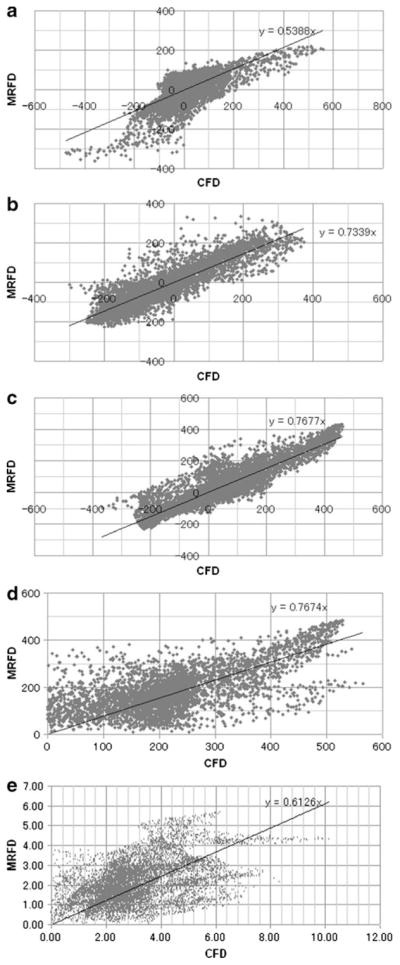
Examples of correlation charts of 3D velocity vector fields and WSS of BA-SCA aneurysm (temporal average) for MRFD and CFD. a X-component of velocity vectors. b Y-component of velocity vectors. c Z-component of velocity vectors. d Magnitude of velocity vectors. e WSS. BA-SCA basilar artery-superior cerebellar artery, WSS wall shear stress, MRFD MR fluid dynamics, CFD computational fluid dynamics

Fig. 3.

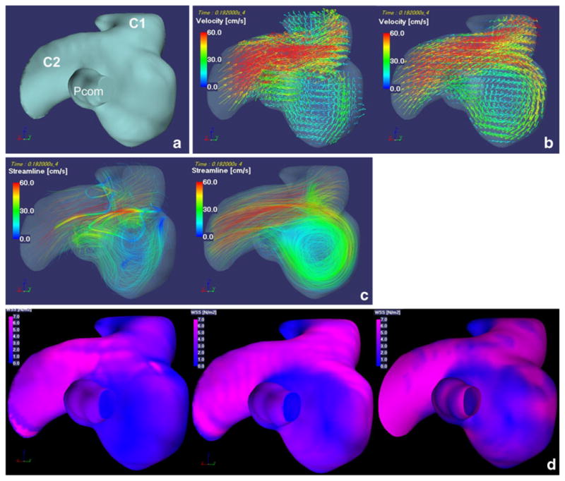
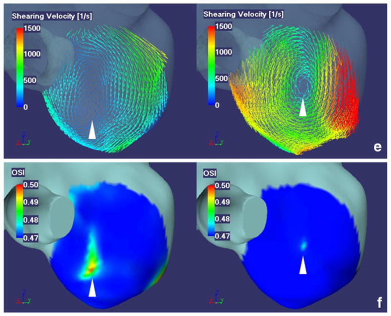
Fifty-one-year-old female with right IC-PC aneurysm with a diameter of 6 mm. a A left posterior oblique view of surface rendered image shows a right IC-PC aneurysm with two outlets. C1 C1 segment of ICA, C2 C2 segment of ICA, Pcom posterior communicating artery. b 3D velocity vector fields (at the systolic phase when the velocities of parent artery is maximum during one cardiac cycle). c 3D streamlines (at the systolic phase when the velocities of parent artery is maximum during one cardiac cycle). d 3D WSS distribution map (temporal average). e Shearing velocity image facing the apex of the spiral flow (temporal average). f 3D OSI maps facing the apex of the spiral flow. Images in b, c, e, f, from the left to the right, present MRFD and CFD. Images in d, from the left to the right, present WSS obtained by MRFD, CFD with the regular interval of the WSS calculation point and the three reference points of 0.575 mm, and WSS by the shearing velocities calculated from the flow velocities of nodes located at the outermost layer of the vasculature (the distance of nodes from the wall, 0.009 mm) in CFD. 3D velocity vector fields (b) and 3D streamlines (c) demonstrate that blood flow enter via the distal aneurysmal neck, rotate very smoothly, and create one spiral flow in the aneurysm. 3D velocity vector fields (b) and 3D streamlines (c) of MRFD and CFD are similar. WSS distribution map (d) obtained from MRFD shows wider area with low WSS around the top of the spiral flow than that from CFD. WSS distribution maps (d) obtained from CFD with the different interval between the calculation point and the reference point(s) are similar. Small and rotating shearing velocities are noted at the top of the spiral flow in the aneurysm (e). This area in MRFD is near that in CFD, however, the magnitude of shearing velocities are different from each other (e). These areas correspond with the high OSI areas (f). IC-PC internal carotid-posterior communicating, ICA internal carotid artery, 3D three-dimensional, WSS wall shear stress, MRFD MR fluid dynamics, CFD computational fluid dynamics, OSI oscillatory shear index

There was also a low to moderate degree of correlation (0.095<R<0.494, P<0.01) between the WSS of aneurysm models obtained with MRFD and CFD (Table 1, Figs. 2 and 3d) by regression analysis. In spite of the difference (0.575 versus 0.009 mm) of the interval of the WSS calculation point and the reference point(s); there was almost no difference of WSS distribution on the aneurysmal surface in the CFD (Fig. 3d).

The small and rotating shearing velocities and higher OSI were observed at the top of the spiral flow of the 3D streamlines (Fig. 3e, f). The location and the extent of these areas in MRFD did not always correspond with those of CFD. However, the center of rotating shearing velocity and high OSI was located in a similar area for both MRFD and CFD

In this study, we used 4D-Flow data set as a boundary condition for CFD. There are almost no differences in correlation efficient against MRFD between CFD using 4D-Flow data set as outlets flow information and CFD without using 4D-Flow data set as outlets flow information (Table 1).

Discussion

Hemodynamics, especially WSS, is thought to play a very important role in the initiation, development, and rupture of intracranial aneurysms. Aneurysms may occur at sites with low and rotating WSS [10] or high WSS [11, 12]. There are two main theories regarding the cause of bleb formation and development or rupture of aneurysms: high WSS [13] or low WSS [11, 14–17]. Other theories focus on flow patterns such as small impingement area on the aneurysmal wall, jet flow, or flow separation causing intimal injury [18–20]. To address these unresolved issues, accurate blood flow information and accurate WSS measurement or accurate WSS calculation are needed.

4D-Flow has the advantage of being able to measure flow velocities in the vessels in living human beings [6–9], although, its spatial resolution and temporal resolution are lower than those of CFD. Accuracy of 4D-Flow has been confirmed using 2D cine PC MR imaging [6]. In this study, we wanted to confirm the accuracy of MRFD using CFD data as a gold standard. We performed regression analysis for 3D velocity vector fields, which showed a moderate to high degree of correlation between MRFD and MR-based CFD (Table 1, Figs. 2 and 3b). The patterns of 3D streamlines were qualitatively well correlated between MRFD and CFD (Fig. 3c). There are several papers comparing velocity vector fields of MRFD obtained by 2D or 3D cine PC MR imaging and LDV or CFD [4, 25–29]. The authors in these papers, however, compare the velocity vectors on a limited number of cine PC MR images with those of CFD, while we compared all velocity vectors in the region of interest with those of corresponding velocity vectors obtained from CFD. Comparative studies [4, 25, 27–29] using 3 T MR scanners or high spatial resolution show better agreements in velocity vector fields between MRFD and LDV or CFD than shown in this study. Our 4D-Flow data set was obtained by a 1.5-T MR scanner and had less signal-to-noise ratio. Perhaps, this was because the larger voxel size of 4D-Flow data used in our study may cause inaccuracy of flow information in each voxel due to partial volume averaging and intravoxel dephasing.

There was a low to moderate degree of correlation between WSS obtained with MRFD and CFD. The degree of the correlation was less in WSS than 3D velocity vector field because WSS was the result of the calculation based on the velocity gradient (derivative value) obtained from the velocity vectors of the reference points, and subtle differences of velocity vectors near the wall were thought to have an enormous effect on the shearing velocity at the wall. WSS measurements were also thought to be sensitive to localization of the wall and slow velocity near the wall. 3D TOF MR angiography might not provide us with accurate geometric information due to slow flow or turbulent flow. 4D-Flow may be susceptible to measurement errors due to slow flow velocities near the wall. Several papers have shown good correlation between MRFD and CFD [26, 29–32]. Unlike previous papers, however, our method compared WSS at all surface points in the region of interest.

The center of rotating shearing velocity and high OSI was located in a similar area for both MRFD and CFD. These points may correspond to the regions with fluctuating WSS at the top of the spiral flow in the aneurysms. These areas may be very important in clinical situations; so, further study is needed.

The time needed for CFD calculation depends on the ability of the computer system, the number of mesh, and the calculation conditions. It takes about 10 h to 2 days. MRFD needed 20 min for MR examination, 170 min for image reconstruction, and less than 1 h for postprocessing. Therefore, MRFD was thought to be a simple and easy method to analyze hemodynamics of intracranial aneurysms. As shown in this study, the results of MRFD were not the same as those obtained by CFD; however, there was a good degree of correlation in 3D velocity vector fields. We thought that MRFD and CFD are complementary methods. We examined five cases, so further study is needed to validate the accuracy of MRFD.

Conclusions

We compared 3D velocity vector fields, 3D streamlines, shearing velocity, WSS, and OSI of five intracranial aneurysms of MRFD using 3D cine PC MR imaging at 1.5 T and MR-based CFD. There was a moderate to high degree of correlation in 3D velocity vector fields and a low to moderate degree of correlation in WSS of intracranial aneurysms between MRFD and CFD. The pattern and location of shearing velocity in MRFD and CFD were similar. The location of high OSI obtained by MRFD was near to that obtained by CFD.

References

- 1.Press W, Teukolsky S, Vetterling W, et al. Numerical recipes in C. Cambridge University Press; Cambridge: 1992. [Google Scholar]
- 2.Malek AM, Alper SL, Izumo S. Hemodynamic shear stress and its role in atherosclerosis. JAMA. 1999;282:2035–2042. doi: 10.1001/jama.282.21.2035. [DOI] [PubMed] [Google Scholar]
- 3.He X, Ku DN. Pulsatile flow in the human left coronary artery bifurcation: average conditions. J Biomech Eng. 1996;118:74–82. doi: 10.1115/1.2795948. [DOI] [PubMed] [Google Scholar]
- 4.Hollnagel DI, Summers PE, Kollias SS, Poulikakos D. Laser Doppler velocimetry (LDV) and 3D phase-contrast magnetic resonance angiography (PC-MRA) velocity measurements: validation in an anatomically accurate cerebral artery aneurysm model with steady flow. J Magn Reson Imaging. 2007;26:1493–1505. doi: 10.1002/jmri.21179. [DOI] [PubMed] [Google Scholar]
- 5.Tateshima S, Tanishita K, Omura H, Villablanca JP, Vinuela F. Intra-aneurysmal hemodynamics during the growth of an unruptured aneurysm: in vitro study using longitudinal CT angiogram database. AJNR Am J Neuroradiol. 2007;28:622–627. [PMC free article] [PubMed] [Google Scholar]
- 6.Markl M, Chan FP, Alley MT, et al. Time-resolved three-dimensional phase-contrast MRI. J Magn Reson Imaging. 2003;17:499–506. doi: 10.1002/jmri.10272. [DOI] [PubMed] [Google Scholar]
- 7.Yamashita S, Isoda H, Hirano M, et al. Visualization of hemodynamics in intracranial arteries using time-resolved three-dimensional phase-contrast MRI. J Magn Reson Imaging. 2007;25:473–478. doi: 10.1002/jmri.20828. [DOI] [PubMed] [Google Scholar]
- 8.Bammer R, Hope TA, Aksoy M, et al. Time-resolved 3D quantitative flow MRI of the major intracranial vessels: initial experience and comparative evaluation at 1.5 T and 3.0 T in combination with parallel imaging. Magn Reson Med. 2007;57:127–140. doi: 10.1002/mrm.21109. [DOI] [PMC free article] [PubMed] [Google Scholar]
- 9.Wetzel S, Meckel S, Frydrychowicz A, et al. In vivo assessment and visualization of intracranial arterial hemodynamics with flow-sensitized 4D MR imaging at 3 T. AJNR Am J Neuroradiol. 2007;28:433–438. [PMC free article] [PubMed] [Google Scholar]
- 10.Mantha A, Karmonik C, Benndorf G, et al. Hemodynamics in a cerebral artery before and after the formation of an aneurysm. AJNR Am J Neuroradiol. 2006;27:1113–1118. [PMC free article] [PubMed] [Google Scholar]
- 11.Shojima M, Oshima M, Takagi K, et al. Magnitude and role of wall shear stress on cerebral aneurysm: computational fluid dynamic study of 20 middle cerebral artery aneurysms. Stroke. 2004;35:2500–2505. doi: 10.1161/01.STR.0000144648.89172.0f. [DOI] [PubMed] [Google Scholar]
- 12.Meng H, Wang Z, Hoi Y, et al. Complex hemodynamics at the apex of an arterial bifurcation induces vascular remodeling resembling cerebral aneurysm initiation. Stroke. 2007;38:1924–1931. doi: 10.1161/STROKEAHA.106.481234. [DOI] [PMC free article] [PubMed] [Google Scholar]
- 13.Hassan T, Timofeev EV, Saito T. Computational replicas: anatomic reconstructions of cerebral vessels as volume numerical grids at three-dimensional angiography. AJNR Am J Neuroradiol. 2004;25:1356–1365. [PMC free article] [PubMed] [Google Scholar]
- 14.Jou LD, Wong G, Dispensa B, et al. Correlation between lumenal geometry changes and hemodynamics in fusiform intracranial aneurysms. AJNR Am J Neuroradiol. 2005;26:2357–2363. [PMC free article] [PubMed] [Google Scholar]
- 15.Jou LD, Lee DH, Morsi H, et al. Wall shear stress on ruptured and unruptured intracranial aneurysms at the internal carotid artery. AJNR Am J Neuroradiol. 2008;29:1761–1767. doi: 10.3174/ajnr.A1180. [DOI] [PMC free article] [PubMed] [Google Scholar]
- 16.Boussel L, Rayz V, McCulloch C, et al. Aneurysm growth occurs at region of low wall shear stress: patient-specific correlation of hemodynamics and growth in a longitudinal study. Stroke. 2008;39:2997–3002. doi: 10.1161/STROKEAHA.108.521617. [DOI] [PMC free article] [PubMed] [Google Scholar]
- 17.Valencia A, Morales H, Rivera R, et al. Blood flow dynamics in patient-specific cerebral aneurysm models: the relationship between wall shear stress and aneurysm area index. Med Eng Phys. 2008;30:329–340. doi: 10.1016/j.medengphy.2007.04.011. [DOI] [PubMed] [Google Scholar]
- 18.Cebral JR, Castro MA, Burgess JE, Pergolizzi RS, Sheridan MJ, Putman CM. Characterization of cerebral aneurysms for assessing risk of rupture by using patient-specific computational hemodynamics models. AJNR Am J Neuroradiol. 2005;26:2550–2559. [PMC free article] [PubMed] [Google Scholar]
- 19.Szikora I, Paal G, Ugron A, et al. Impact of aneurysmal geometry on intraaneurysmal flow: a computerized flow simulation study. Neuroradiology. 2008;50:411–421. doi: 10.1007/s00234-007-0350-x. [DOI] [PubMed] [Google Scholar]
- 20.Ohshima T, Miyachi S, Hattori K, et al. Risk of aneurysmal rupture: the importance of neck orifice positioning-assessment using computational flow simulation. Neurosurgery. 2008;62:767–773. doi: 10.1227/01.neu.0000318160.59848.46. [DOI] [PubMed] [Google Scholar]
- 21.Shimai H, Yokota H, Nakamura S, et al. Extraction from biological volume data of a region of interest with non-uniform intensity. In: Sumi Kazuhiko., editor. Optomechatronic Machine Vision; Proceedings of SPIE; 2005. p. 605115. [Google Scholar]
- 22.Lorensen WE, Cline HE. Marching cubes: a high resolution 3D surface construction algorithm. Comput Graph. 1987;21:163–169. [Google Scholar]
- 23.Masaryk AM, Frayne R, Unal O, et al. In vitro and in vivo comparison of three MR measurement methods for calculating vascular shear stress in the internal carotid artery. AJNR Am J Neuroradiol. 1999;20:237–245. [PMC free article] [PubMed] [Google Scholar]
- 24.Cheng CP, Parker D, Taylor CA. Quantification of wall shear stress in large blood vessels using Lagrangian interpolation functions with cine phase-contrast magnetic resonance imaging. Ann Biomed Eng. 2002;30:1020–1032. doi: 10.1114/1.1511239. [DOI] [PubMed] [Google Scholar]
- 25.Zhao SZ, Papathanasopoulou P, Long Q, Marshall I, Xu XY. Comparative study of magnetic resonance imaging and image-based computational fluid dynamics for quantification of pulsatile flow in a carotid bifurcation phantom. Ann Biomed Eng. 2003;31:962–971. doi: 10.1114/1.1590664. [DOI] [PubMed] [Google Scholar]
- 26.Marshall I, Zhao S, Papathanasopoulou P, Hoskins P, Xu Y. MRI and CFD studies of pulsatile flow in healthy and stenosed carotid bifurcation models. J Biomech. 2004;37:679–687. doi: 10.1016/j.jbiomech.2003.09.032. [DOI] [PubMed] [Google Scholar]
- 27.Canstein C, Cachot P, Faust A, et al. 3D MR flow analysis in realistic rapid-prototyping model systems of the thoracic aorta: comparison with in vivo data and computational fluid dynamics in identical vessel geometries. Magn Reson Med. 2008;59:535–546. doi: 10.1002/mrm.21331. [DOI] [PubMed] [Google Scholar]
- 28.Karmonik C, Klucznik R, Benndorf G. Comparison of velocity patterns in an AComA aneurysm measured with 2D phase contrast MRI and simulated with CFD. Technol Health Care. 2008;16:119–128. [PubMed] [Google Scholar]
- 29.Marshall I, Zhao S, Papathanasopoulou P, et al. MRI and CFD studies of pulsatile flow in healthy and stenosed carotid bifurcation models. J Biomech. 2004;37:679–687. doi: 10.1016/j.jbiomech.2003.09.032. [DOI] [PubMed] [Google Scholar]
- 30.Moore JA, Steinman DA, Holdsworth DW, Ethier CR, et al. Accuracy of computational hemodynamics in complex arterial geometries reconstructed from magnetic resonance imaging. Ann Biomed Eng. 1999;27:32–41. doi: 10.1114/1.163. [DOI] [PubMed] [Google Scholar]
- 31.Papathanasopoulou P, Zhao S, Köhler U, et al. MRI measurement of time-resolved wall shear stress vectors in a carotid bifurcation model, and comparison with CFD predictions. J Magn Reson Imaging. 2003;17:153–162. doi: 10.1002/jmri.10243. [DOI] [PubMed] [Google Scholar]
- 32.Ahn S, Shin D, Tateshima S, Tanishita K, Vinuela F, Sinha S. Fluid-induced wall shear stress in anthropomorphic brain aneurysm models: MR phase-contrast study at 3 T. J Magn Reson Imaging. 2007;25:1120–1130. doi: 10.1002/jmri.20928. [DOI] [PubMed] [Google Scholar]