

Abstract
The class of autocalibrating “data-driven” parallel imaging (PI) methods has gained attention in recent years due to its ability to achieve high quality reconstructions even under challenging imaging conditions. The aim of this work was to perform a formal comparative study of various data-driven reconstruction techniques to evaluate their relative merits for certain imaging applications. A total of five different reconstruction methods are presented within a consistent theoretical framework and experimentally compared in terms of the specific measures of reconstruction accuracy and efficiency using one-dimensional (1D)-accelerated Cartesian datasets. It is shown that by treating the reconstruction process as two discrete phases, a calibration phase and a synthesis phase, the reconstruction pathway can be tailored to exploit the computational advantages available in certain data domains. A new “split-domain” reconstruction method is presented that performs the calibration phase in k-space (kx, ky) and the synthesis phase in a hybrid (x, ky) space, enabling highly accurate 2D neighborhood reconstructions to be performed more efficiently than previously possible with conventional techniques. This analysis may help guide the selection of PI methods for a given imaging task to achieve high reconstruction accuracy at minimal computational expense.
Keywords: parallel imaging, autocalibrating, GRAPPA, reconstruction, MRI
Over the last decade, parallel imaging (PI) technology in MRI has progressed from early research prototype to established clinical tool. PI accelerates data acquisition by exploiting the spatial dependence of phased-array receiver coil sensitivity. This acceleration has been used to satisfy a variety of imaging objectives, including reduced scan time, decreased image artifacts, increased spatial resolution, greater volumetric coverage, or some combination of the above, depending on the specific application.
Many different PI techniques have been developed to date. While most methods employ the same approach of accelerating data acquisition by using coil sensitivity encoding to supplement gradient encoding, they differ in how they solve the reconstruction problem to generate the final, unaliased image. Existing PI methods can be divided into two classes based on how they model the reconstruction. The first class consists of methods that require explicit knowledge of the coil sensitivity functions in order to separate aliased signals, including methods such as sensitivity encoding (SENSE) (1), modified SENSE (mSENSE) (2), simultaneous acquisition of spatial harmonics (SMASH) (3), and sensitivity profiles from an array of coils for encoding and reconstruction in parallel (SPACE RIP) (4), among others (5,6). We refer to this class of PI methods as “physically-based” reconstructions because they closely model the underlying physical process that occurs during image acquisition. However, images reconstructed with physically-based methods can suffer from artifacts caused by inaccuracies in coil sensitivity calibration. Common sources of calibration error include insufficient signal-to-noise ratio (SNR), Gibbs ringing, motion, or tight field-of-view (FOV) prescription (7,8).
The second class of PI methods does not require explicit coil sensitivity information but rather uses a data fitting approach to calculate the linear combination weights that reconstruct output or “target” data from neighboring input or “source” data. We refer to this second class of methods as “data-driven” reconstructions because they are based on a limited knowledge of the underlying physical process and rely on training data to calibrate the relationship between input and output data. This class of methods includes AUTO-SMASH (9), variable density AUTO-SMASH (VD-AUTO-SMASH) (10), and generalized autocalibrating partially parallel acquisitions (GRAPPA) (11), among others (12–14). Data-driven methods such as GRAPPA that perform a coil-by-coil reconstruction offer improved image quality over those that generate a composite-coil complex sum image such as VD-AUTO-SMASH owing to the lack of phase cancellation effects (11). Furthermore, because they require no sensitivity maps, coil-by-coil data-driven (CCDD) methods can be advantageous compared to physically-based methods for situations in which accurate coil sensitivity estimation is difficult (7).
Even among the subset of CCDD reconstructions, a variety of different methods have been proposed. In general, CCDD reconstructions can be described as generating skipped data on a single coil via a linear combination of neighboring data on all coils, with the linear combination weights determined by fitting to fully sampled training data, or autocalibrating signals (ACS). However, the particular approach used to derive and apply the weights varies significantly from one method to another. Given the variety of CCDD reconstruction approaches, the question arises as to how one might choose a particular method from among these choices. The goal of this work was to perform a formal comparison of five types of CCDD reconstruction methods to evaluate their relative merits for certain imaging applications. A complete analysis of a given reconstruction method should consider both its reconstruction accuracy as well as its computational efficiency. Reconstruction accuracy plays a chief role in determining final image quality, whereas computational efficiency impacts software and hardware requirements, total reconstruction time, and ease of integration into routine practice. While the ideal method would optimize both parameters, tradeoffs must sometimes be made in favor of one parameter or the other depending on the application. Thus all CCDD methods under consideration were compared in terms of the specific measures of reconstruction accuracy and efficiency to identify the relevant practical differences between methods. Based on this analysis, a flexible method is proposed for tailoring the CCDD reconstruction pathway to exploit the computational advantages available in certain data domains.
THEORY
This section presents the theoretical framework for five different CCDD methods evaluated in this work, using a consistent notation to enable quantitative and qualitative comparisons. All five reconstruction methods are assumed to share the same general acquisition scheme shown in Fig. 1a, whereby multicoil k-space data collection is accelerated by a reduction factor R by acquiring only every Rth phase-encode line on a Cartesian grid. (Throughout this work, we assume data sampling on a Cartesian grid only.) A small number of ACS lines are additionally acquired to form a fully sampled calibration region, indicated by region II in Fig. 1a. The acquisition of calibration lines can either be embedded within the accelerated scan itself, or performed before or after accelerated data collection. The former approach is commonly used because it minimizes artifacts from misregistration. For purposes of this work, the analysis is restricted to acceleration in only one dimension, although the results could also be extended to 2D acceleration, i.e., acceleration in both phase-encoding directions in 3D imaging.
FIG. 1.

a: Example data acquisition pattern in which k-space data from each of four coils is accelerated by acquiring every other phase-encode line (R = 2). Additional ACS lines are acquired in the central k-space region, forming the fully sampled calibration region denoted II. The outer k-space regions, denoted I, are undersampled by reduction factor R. b–f: Spatial representation of the reconstruction weights generated by Methods 1–5, assuming the sampling pattern in a. The green dots represent the linear combination weights that are applied to source data at the corresponding locations in the same data space to synthesize data on a single coil at the location indicated by the magenta dot. b: Method 1 uses a 1D neighborhood of width Dy in the ky-direction that can be calculated in either (x, ky) or (kx, ky) space. c: In Method 2, unique 1D neighborhood reconstruction weights are calculated for each x-location in hybrid (x, ky) space. d: Method 3 extends the reconstruction to a 2D k-space neighborhood of size [Dy × dx]. e: Method 4 begins with the same 2D k-space weights as Method 3, then zero-pads to full size and performs a 2DFT to transform the weights into (x, y) image space. f: Method 5 also begins with a 2D k-space weights, then zero-pads to full size in kx, followed by a 1DFT to transform the weights into hybrid (x, ky) space such that a unique set of weights exists at each x-location.
CCDD reconstruction can be conceptually divided into two discrete processing phases: 1) a “calibration phase,” in which the linear combination weights that fit known source data to known target data are calculated using fully sampled calibration data as a training guide (region II in Fig. 1a); and 2) a “synthesis phase,” in which unacquired data (region I in Fig. 1a) is synthesized from acquired data using the reconstruction weights derived in the calibration phase. This division into two processing phases is important because the various CCDD methods differ in their treatment of each phase. Specifically, the particular data domain or space (i.e., k-space, hybrid-space, or image space) in which each phase occurs can vary from one CCDD method to the next, leading to differences in reconstruction accuracy and efficiency. The five types of CCDD reconstructions analyzed in this work are summarized as follows:
Method 1: k-Space-based 1D neighborhood CCDD reconstruction
- Method 2: Hybrid-space-based CCDD reconstruction, including three different calibration schemes:
- Calibration A: independent calibration
- Calibration B: segmented calibration
- Calibration C: smoothly varying calibration
Method 3: k-Space-based 2D neighborhood reconstruction
Method 4: k-Space-calibration, image-space synthesis CCDD reconstruction
Method 5: k-Space calibration, hybrid-space synthesis CCDD reconstruction
FIG. 2.

(left column) Images generated using five different CCDD reconstruction methods on the same 1D-accelerated brain phantom dataset (R = 3). (right column) Reconstruction error images (window/level decreased by 10×). a, f: Method 1. b, g: Method 2A. c, h: Method 2B. d, i: Method 2C. e, j: Methods 3, 4, and 5 generated identical images. Phase-encode direction is horizontal, and ACS lines were removed from the final images.
For each method, the general reconstruction model is first presented, followed by details of calibration and synthesis phase calculation. An estimate of computational expense is calculated as the number of basic operations needed to perform the dominant or “rate-limiting” step in each reconstruction phase.1 For simplicity, we chose to define a basic unit of operation as a single complex-valued multiplication. Measuring computational efficiency in terms of operations rather than computation time allowed us to compare methods strictly on the basis of computational complexity and avoid dependencies on system-specific variables such as computer platform, compiler, coding routines, etc. Furthermore, expressing computational cost as a function of imaging and reconstruction variables helps predict how the computation scales as those parameters are varied. The computational expense calculation included all CCDD reconstruction steps required to convert an initial accelerated dataset into a final unaliased dataset, including the calibration phase, weight conversion (if necessary), and synthesis phase. However, the cost associated with performing the two 1D Fourier transforms (FT) (one in kx, one in ky) necessary to transform k-space data into image space, as well as the cost to perform coil combination or any other subsequent data processing steps, were excluded since all reconstructions were assumed to share these steps in common. A validation of the theoretical computational expense estimates is deferred to a later section.
Method 1: k-Space-Based 1D-Neighborhood CCDD Reconstruction
The original CCDD reconstruction, GRAPPA (11), was formulated as a 1D-neighborhood reconstruction performed entirely in k-space. The underlying assumption of GRAPPA is that every k-space data point on a single coil can be represented as a linear combination of its neighbors on all coils and that the set of linear combination weights is shift invariant in k-space. The signal at each skipped k-space location from coil n was modeled as follows (adapted from Griswold et al. (11)):
| (1) |
where R is the acceleration factor, r is the phase-encode offset from an acquired reference line to an unacquired line (r = 1, … , R − 1), Δky is the distance from one phase-encode line to the next, index j counts through Nc individual coils, and index τy spans dy acquired points within a local 1D neighborhood along the ky direction. Wn,r,j(τy) represents the weight applied to acquired k-space data at phase-encode offset location τyR on coil j to reconstruct data at phase-encode offset location r on coil n. The local 1D neighborhood has width Dy (Dy = (dy − 1)*R + 1) and can either be centered symmetrically about the missing data point or shifted asymmetrically to one side. Throughout this work, a single, symmetric neighborhood is assumed (as opposed to a sliding block reconstruction (11) or other asymmetric neighborhood formulation). An illustration of the 1D neighborhood weights for Method 1 is shown in Fig. 1b.
We can rewrite the reconstruction model in Eq. [1] in compact matrix form as follows:
| (2) |
where contains the synthesized data generated by linearly combining the acquired data points in Sacq with the reconstruction weights in W. Whereas the summation formulation in Eq. [1] describes only the synthesis of a single data point at a particular phase-encode offset location r on coil n, the matrix formulation in Eq. [2] can conveniently be written to encompass the synthesis of all R − 1 phase-encode offset locations on all Nc coils. The matrix assembly procedures are described in detail below.
Calibration
The weight matrix W used in the reconstruction must be derived during an initial calibration phase by finding a solution to the linear system
| (3) |
where the matrices Ssrc and Stgt are comprised of known source and target data, respectively, taken from the fully sampled calibration region. The weights in W can be found to minimize the error ε1 in the fit between source and target data as follows:
| (4) |
where ∥·∦2 denotes the L2 norm. The position of source points with respect to target points matches the sampling pattern encountered in the accelerated regions of k-space. For each of Nt available target points in the calibration region, the corresponding dy source points that fall within the local 1D neighborhood of width Dy along the ky direction are identified on all coils and assembled into a row of Ssrc. The target points for a given coil and phase-encode offset location are assembled into a column of Stgt. Thus matrix Ssrc has dimension [Nt × dyNc], matrix Stgt has dimension [Nt × (R − 1)Nc], and matrix W has dimension [dyNc × (R − 1)Nc].
The total number of target points Nt represents the number of training examples for the reconstruction. Generally, the greater the number of training examples, the more accurate the fitting process becomes in the presence of noise (10). Furthermore, even in the absence of noise, additional training examples can allow improved characterization of how the coil sensitivity functions relate to the local neighborhood. The acquisition of multiple ACS lines, originally proposed in Ref. 10, serves to increase the number of available target points at the expense of acquisition efficiency. A “floating net” calibration approach, as defined in Ref. 13, can also be used to take full advantage of all available target points along ky. In addition, since the reconstruction is shift invariant, the calibration can be performed at all Nx locations along the kx direction (15), further increasing Nt; we refer to such a calibration strategy as “full-width readout calibration.” Fewer than Nx samples could be used to reduce computation time, but for this work, full-width readout calibration is assumed. If we define Nf as the number of possible fit locations along the phase-encode direction, then the total number of target points Nt equals NfNx, a number that can easily exceed several thousand for typical scan parameters. As a result, the linear system to be solved is highly overdetermined (Nt ⪢ dyNc). Thus W can be calculated using a least-squares fitting approach:
| (5) |
where + denotes the pseudoinverse and H the conjugate transpose. When Nt is large, performing the series of matrix multiplications specified in Eq. [5] can require a substantial number of computations. By taking advantage of the associative property of matrix multiplication, we can rewrite Eq. [5] as
| (6) |
which simplifies the computation by removing the Nt dimension from the product . It can be shown that the dominant calibration cost of Method 1 is the calculation of , which requires NfNx(Ncdy)2 complex-valued multiplications.
Synthesis
In the synthesis phase, the missing data is synthesized according to Eq. [2], where each row of matrix Sacq contains the acquired points within a local 1D neighborhood about a given unacquired point on all coils, each column of matrix W contains the precalculated weights, and each column of matrix Sacq consists of Ns total points to be synthesized for a given coil (Ns = NuNx, where Nu is the number of phase-encode lines to be synthesized at a particular phase-encode offset location). Thus matrix Sacq has dimension [NuNx × dyNc], matrix Ssyn has dimension [NuNx × (R − 1)Nc], and matrix W has dimension [dyNc × (R − 1)Nc]. Accordingly, the cost to synthesize Nc complete k-space datasets is dyNuNxN2c(R − 1) multiplications. If desired, the ACS lines can be retained in the final datasets for improved image quality and SNR (10,11).
From the foregoing description, it can be seen that both the training and synthesis phases of Method 1 are performed in k-space. Thus, GRAPPA has historically been referred to as a “k-space reconstruction.” However, it should be noted that due to system linearity and Fourier transform separability, Method 1 can equivalently be performed in a hybrid (x, ky) space into which data has been transformed via 1D FT along kx (FTkx):
| (7) |
where S′ denotes the acquired signal transformed into hybrid (x, ky) space. Otherwise all steps in the calibration and synthesis phases would remain the same as described above. For a 1D neighborhood CCDD reconstruction, the weights Wn,r,j(τy) will be the same in either (kx, ky) space or in hybrid (x, ky) space because they have no dependency on the transformed direction. While there is no reconstruction accuracy or efficiency advantage to performing Method 1 in hybrid-space, it is mentioned here for completeness. More sophisticated hybrid-space reconstruction methods that model x-position dependency are described in the next section.
Method 2: Hybrid-Space-Based CCDD Reconstruction
More recent studies have formulated the entire CCDD reconstruction not in (kx, ky) space but rather in hybrid (x, ky) space. These hybrid-space techniques model the reconstruction as:
| (8) |
where W′n,r,j(x,τy) denotes the hybrid-space reconstruction weights, which now contain a dependency on x. In this case, a unique set of linear combination weights exists at each x-location, as shown in Fig. 1c. By allowing variable reconstruction weights along the x-direction, this hybrid-space formulation can offer better system conditioning and image quality compared to Method 1. The synthesis and calibration phases for Method 2 can similarly be written in the compact matrix form of Eqs. [2] and [3], respectively, except with the signal and weight matrices composed of data in hybrid-space.
A number of different calibration strategies have been presented for generating hybrid-space reconstruction weights with x-dependency. Three of these calibration strategies are described below.
Calibration A: Independent Calibration
One calibration option is to calculate a unique set of reconstruction weights independently for each x-location (16). In this case, the number of target points Nt is limited to Nf, the number of fit locations at a single x-position, which generally results in an underdetermined (Nf < dyNc), critically determined (Nf = dyNc), or only slightly overdetermined (Nf > dyNc) problem, which in practice can lead to poor quality reconstructions. Although it is possible to increase the number of ACS lines to improve system determination, this reduces net acceleration. Using this “independent calibration” approach, a weight matrix W of size [dyNc × (R − 1)Nc] can be calculated for each x-location using Eq. [5] (which is now more efficient than Eq. [6] because Nt is small), with matrix Ssrc of size [Nf × dyNc] and matrix Stgt of size [Nf × (R−1)Nc]. The estimated cost to perform this calibration requires NfNx(Ncdy)2 multiplications to compute SHsrcSsrc a total of Nx times, not to mention Nx matrix inversions—one for every x-location. For the purpose of this work, it suffices to say that the computational cost for this approach is greater than for Method 1.
Calibration B: Segmented Calibration
Another method for generating hybrid-space weights that has been mentioned in the literature (17–19) divides the x-direction into Nseg segments over which the reconstruction weights are assumed to remain constant, improving system determination by increasing the number of training examples by the width of the segment (Nt = NfNx/Nseg). The basic assumption is that coil sensitivity varies slowly in the spatial domain (i.e., over the x-direction) and therefore reconstruction weights can be approximated as having fixed values over discrete segments along this axis. Using this “segmented calibration” scheme, we can write the hybrid-space weights in Eq. [8] as
| (9) |
where:
indicating an even step-wise weight variation over x. Another version of segmented calibration uses overlapping segments followed by interpolation of weights between segments (19).
A weight matrix W of size [dyNc × (R − 1)Nc] can be calculated for each segment using either Eq. [5] or [6] (the more computationally efficient choice will depend on the size of Nt), where matrix Ssrc has dimension [NfNx/Nseg × dyNc] and matrix Stgt has dimension [NfNx/Nseg × (R−1)Nc]. In either case, the computation required for segmented calibration will again be at least as great as that reported for Method 1, requiring NfNx(Ncdy)2 multiplications to compute SHsrcSsrc a total of Nseg times, as well as Nseg matrix inversions.
Calibration C: Smoothly Varying Calibration
A third hybrid-space calibration method has been shown to improve upon the accuracy of both independent and segmented calibration by modeling the weights as smoothly varying functions of x (14,19). Rather than estimating the weights independently over discrete segments, “smoothly varying calibration” considers all data along x simultaneously and relates the weights to one another with continuous weight functions. Smoothly varying hybrid-space weights can be modeled as a linear combination of Norder terms of a basis function, as follows:
| (10) |
where represents the coefficient for the cxth term (cx = 0,… Norder) of basis function f(x,cx). A variety of basis functions could be used. As described in Skare and Bammer (14), smoothly varying weight functions can be represented in compact matrix form:
| (11) |
where Q is the fixed and sparse basis set matrix of size [dyNxNc × NcdyNorder], H is the coefficient matrix of size [NcdyNorder × (R − 1)Nc], and W’ is the weight matrix of size [dyNxNc × (R − 1)Nc]. In the calibration phase, rather than calculating the weights W’ directly, the basis function coefficient matrix H is derived by finding a solution to the linear system
| (12) |
The solution that minimizes the error ε2 can be found by evaluating the following least-squares expression:
| (13) |
where the sparse matrices Ssrc and Stgt are comprised of hybrid-space source and target data and have sizes [NfNx × dyNxNc] and [NfNx × (R−1)Nc], respectively.
The dominant term in evaluating Eq. [13] is the multiplication of (SsrcQ)H by (SsrcQ), which requires NfNx-(NcdyNorder)2 multiplications—a factor of Norder2 more computations than the corresponding step for Method 1. To this one must add the cost of calculating both the product SsrcQ as well as the product QH to find the final weight matrix W’ in Eq. [11]. Although these steps can be performed fairly efficiently due to matrix sparsity, they nevertheless add extra complexity to calibration phase computation.
Synthesis
No matter what calibration method is used, the application of the weights in the synthesis phase is similar for all for hybrid-space methods. Synthesis can be performed by evaluating the matrix expression in Eq. [2] for each x-location, where each row of matrix Sacq contains the acquired hybrid-space data from all coils within a local 1D neighborhood of an unacquired point, and each column of matrix W contains the precalculated hybrid-space weights for that x-location. Thus matrix Sacq has dimension [Nu × dyNc] and matrix W has dimension [dyNc × (R − 1)Nc]. (W’ in Calibration C can be recast into Nx matrices of dimension [dyNc × (R − 1)Nc] to take the form of W.) Accordingly, the cost to synthesize Nc complete hybrid-space datasets is dyNuNxN2c(R − 1), which is the same computation required for the synthesis step for Method 1. The ACS lines can be retained in the final hybrid-space datasets for improved image quality and SNR.
Method 3: k-Space-Based 2D-Neighborhood CCDD Reconstruction
Several authors have demonstrated a variation on k-space-based CCDD reconstruction whereby the local neighborhood is expanded to 2D to include data along both the phase- and frequency-encode directions (12,13,20,21). Extending the formulation in Eq. [1], the signalŜ at each skipped k-space location from coil n can be written as a linear combination of neighboring acquired data along the kx and ky directions from all coils:
| (14) |
where the reconstruction weights Wn,r,j(τx,τy) contain an additional dependence on position index τx, which spans dx acquired points along the kx direction. A graphical illustration of 2D neighborhood k-space weights is shown in Fig. 1d. As before, Eq. [14] can be rewritten in the compact matrix form of Eq. [2], where Sacq now consists of the acquired data within the local 2D neighborhood that when linearly combined using the weights in W will synthesize data in Ŝsyn.
Calibration
During the calibration phase, the reconstruction weights in matrix W are found by solving Eq. [4], where the matrices Ssrc and Stgt are comprised of source and target k-space data, respectively. For each possible target point location in the calibration region, the corresponding dxdy source points that fall within the local 2D neighborhood of width [dx × Dy] are identified on all coils and assembled into a row of Ssrc. The target points for a given coil are assembled into a column of Stgt. Thus matrix Ssrc has dimension [NfNx × dxdyNc] and matrix Stgt has dimension [NfNx × (R − 1)Nc].
While the number of unknown weights in Method 3 is greater than in Method 1 owing to the inclusion of source data along the kx dimension, the system is still typically overdetermined (Nt ⪢ dxdyNc), especially if full-width readout calibration is used. Thus the reconstruction weights W can be calculated using Eq. [6]. In this case, the dominant term in evaluating Eq. [6] is the computation of SHsrcSsrc, which requires NfNx(Ncdxdy)2 complex-valued multiplications, or dx2 times more computations than the same step in Method 1.
Synthesis
In the synthesis phase, the missing k-space data are synthesized from local acquired data by evaluating Eq. [2], where each row of matrix Sacq is comprised of acquired points within a local 2D neighborhood about a given unacquired point on all coils, and matrix W contains the precalculated weights. Thus matrix Sacq has dimension [NuNx × dxdyNc] and matrix W has dimension [dxdyNc × (R − 1)Nc]. Accordingly, the cost to synthesize Nc complete k-space datasets is dxdyNuNxNc2(R − 1), or dx × more computations than the synthesis step in Methods 1 or 2. The ACS lines can be retained in the final k-space datasets.
Method 4: k-Space Calibration, Image-Space Synthesis CCDD Reconstruction
All of the foregoing CCDD reconstruction methods perform both the calibration and synthesis phases in the same data space: Methods 1 and 3 were entirely performed in k-space, while Method 2 was performed entirely in hybrid-space. We now turn our attention to “split-domain” approaches that perform the calibration and synthesis phases in different data domains.
Several authors have noted that k-space-based CCDD reconstructions can be viewed as convolution operations (15,18,20,22). The 2D-neighborhood k-space reconstruction model used in Eq. [14] can be reformulated as the following discrete 2D convolution sum (23):
| (15) |
where is a 2D k-space convolution kernel with indices Ωx and Ωy spanning a 2D neighborhood of size [dx × Dy]. The convolution kernel can be formed from the reconstruction weights Wn,r,j(τx,τy) from Eq. [14] by filling zeroes in the appropriate unacquired locations to match the accelerated sampling pattern. In addition, for the set of kernels for which the source and target data are on the same coil (i.e., j = n), the weight at the synthesis location should be set to 1 for the convolution to retain the original k-space lines for that coil. The 2D convolution operation assumes that S is uniformly sampled in both the kx and ky directions, a condition that can be achieved by ensuring the ACS lines are removed from S prior to data synthesis.
As previously mentioned (18,20), expressing the reconstruction as a convolution allows one to easily extend the CCDD technique from k-space to image-space. According to Fourier theory (23), Eq. [15] can be converted into image-space via 2D FT as follows:
| (16) |
where w is the set of weights obtained by centering and zero-padding the k-space convolution kernel W̃ up to size [Nx × Ny] and performing a 2DFT, and s is the aliased image of size [Nx × Ny], obtained by zero-filling the unacquired k-space points in S and performing a 2DFT. While performing a multiplication in image space is mathematically equivalent to a 2D convolution in k-space (assuming circular convolution is employed at the k-space boundaries), it can offer computational advantages because a point-by-point multiplication is more efficient than a 2D convolution, as enumerated below. A diagram of image-based reconstruction weights derived from 2D k-space weights is shown in Fig. 1e.
Calibration
Because the calibration phase for Method 4 is performed in k-space, the estimated cost for the calculation of k-space weights is identical to Method 3 (assuming a 2D kernel neighborhood is used), namely NfNx(Ncdxdy)2 complex-valued multiplications. However, one must also include the nontrivial additional cost of converting the k-space weights to image-space: after zero-padding to size [Ny × Nx], two fast Fourier transforms (FFTs) can be performed (each of order NlogN), requiring a total of (logNx + logNy)NxNyNc2 operations for all coils.
Synthesis
The synthesis phase of Method 4 consists of performing the point-by-point multiplication in Eq. [16] for each coil n and phase-encode offset r, requiring a total of NxNyNc2(R − 1) multiplications to reconstruct Nc individual coil images. A primary disadvantage of image-space synthesis is the requirement that acquired data be uniformly undersampled, precluding the reconstruction of nonuniform sampling patterns (for example, if different integer acceleration factors are used in different k-space regions) and necessitating the removal of ACS lines prior to image-space synthesis.
Method 5: k-Space Calibration, Hybrid-Space Synthesis CCDD Reconstruction
With Method 5, we introduce a split-domain approach that improves upon the computational efficiency of Method 3 while preserving its flexibility to reconstruct non-uniform sampling patterns (24). Returning to the 2D k-space reconstruction model of Method 3, we perform a 1D FT along the fully sampled kx-direction to transform Eq. [14] into hybrid (x, ky) space:
| (17) |
which can be shown to reduce to:
| (18) |
where
| (19) |
Equations [17]–[19] imply that 2D reconstruction weights Wn,r,j(τx,τy) can be found in k-space, zero-padded in kx and 1D Fourier transformed into hybrid-space, then applied to accelerated data that has similarly been transformed into hybrid-space. A diagram of hybrid-space weights derived from 2D k-space weights in this manner is shown in Fig. 1f. While performing data synthesis as a 1D linear combination in hybrid-space is mathematically equivalent to performing a 2D linear combination in k-space (assuming circular k-space boundary conditions are employed), it offers computational advantages owing to the reduction in neighborhood dimension. Moreover, unlike Method 4, since the phase-encode direction remains in ky-space, the ACS lines can be retained in the final hybrid-space dataset.
One may note that the hybrid-space synthesis equation of Method 5 (Eq. [18]) is identical to that of Method 2 (Eq. [8]). The two methods differ in how they arrive at the hybrid-space reconstruction weights: Method 2 calculates the reconstruction weights in hybrid-space using one of several calibration strategies, whereas Method 5 calculates 2D weights in k-space and then transforms them into hybrid-space via 1DFT. As described in Eq. [10], when the calibration strategy of Method 2C is used, the hybrid-space weights are modeled with a basis function f to enforce smoothly varying weights over x. Comparing that equation with the hybrid-space weight derivation used in Eq. [19], it becomes apparent that these two equations take very similar forms. In fact, if a complex exponential basis function is used for f (as proposed in (19)), and Wn,r,j(τx,τy) and cx span the same number of terms, then the two equations are equivalent. From this perspective, solving for the 2D neighborhood weights Wn,r,j(τx,τy) in k-space can be viewed as finding the complex Fourier series coefficients that generate a smoothly varying weight function in hybrid-space, and vice versa.
Calibration
The theoretical cost to calculate 2D neighborhood k-space weights for Method 5 is NfNx(Ncdxdy)2 multiplications, identical to that of Method 3. After zero-padding to size [dy × Nx], the additional cost of converting the k-space weights to hybrid-space via 1D FFT along the x dimension amounts to (NxlogNx)dyNc2 operations.
Synthesis
The synthesis phase for Method 5 is identical to Method 2, requiring dyNuNxNc2(R − 1) multiplications to synthesize Nc hybrid-space datasets. The fully sampled ACS lines can be retained in the final hybrid-space dataset.
METHODS
Reconstruction Accuracy Measurements
A series of experiments were performed to compare the reconstruction accuracy of CCDD methods. Because reconstruction performance depends on several factors such as coil geometry, subject, and acceleration factor, we performed phantom and in vivo experiments using two different imaging configurations. First, a 2D fast spin echo axial dataset of a brain phantom (Hoffman 3-D Brain Phantom™, Data Spectrum, Chapel Hill, NC, USA) was acquired on a 1.5T Signa HD scanner (GE Healthcare, Waukesha, WI, USA) using an eight-channel head coil (MRI Devices, Pewaukee, WI, USA) (eight-coil elements arranged circularly about a cylinder) with the following imaging parameters: TE/TR = 13 ms/400 ms, FOV = 21 cm, bandwidth (BW) =±16 kHz, slice thickness = 4 mm, 240 × 240 pixels. The phantom dataset was retrospectively downsampled by a reduction factor of R = 3, and ACS lines at the k-space center were retained for a fully sampled calibration region spanning 20 phase-encode lines.
Next, an axial 3D fat-suppressed gradient echo volunteer abdominal dataset was acquired using an eight-channel torso array coil (GE Healthcare) (2 × 2 anterior coil elements and 2 × 2 posterior elements) with the following imaging parameters: TE/TR = 2.2 ms/4.6 ms, FOV = 36 cm, BW = ±62 kHz, slice thickness = 3 mm, matrix size = 320 × 256 × 60. This dataset was retrospectively downsampled by R = 2 in the phase-encode direction and included a fully sampled central region spanning 20 phase-encode lines. Volunteer scanning was approved by our Institutional Review Board and was performed with informed consent.
CCDD Methods 1 through 5, including all three calibration variations for Method 2, were implemented in Matlab 7.0 (The Mathworks, Inc, Natick, MA, USA) and used to reconstruct both datasets according to the details in the Theory section, with floating net calibration in ky, full-width readout calibration in kx (where applicable), and a single, symmetric neighborhood about the target point with two neighbors in the ky direction (dy = 2). For 2D neighborhood k-space calibration, a neighborhood width of five was used in the kx direction (dx = 5); for segmented hybrid-space calibration (Method 2B), eight independent, nonoverlapping segments were used along the x-direction (Nseg = 8); for smoothly varying hybrid-space calibration (Method 2C), the weights over x were modeled according to Eq. [10] using the following cosine basis function:
| (20) |
Where applicable, circular boundary conditions were assumed at the edges of k-space. For each dataset, the same number of ACS lines was used with all methods to compare reconstruction results based on equivalent net acceleration. For Method 4, the ACS lines were necessarily removed prior to image-based synthesis to achieve a uniform sampling pattern. Thus to enable a fair comparison among different CCDD methods, the ACS lines were similarly removed from all datasets prior to synthesis.
An accelerated coil-combined image was reconstructed for each CCDD method, and a reconstruction error image was calculated as the magnitude of the difference between the unaccelerated reference image and the accelerated image. In an attempt to quantify the reconstruction performance of each method, a net reconstruction error was calculated as the relative root mean squared (RRMS) error between the unaccelerated and accelerated image, normalized by the signal intensity of the reference image, as used in previous work (25,26):
| (21) |
where M is the total number of pixels in the image, Ireference is the reference image, and Irecon is the reconstructed image.
Reconstruction Efficiency Measurement
To experimentally validate the theoretical computational expense estimates reported in the Theory section, measurements of actual computation times were compared for a subset of CCDD methods. Because of the considerable computational overhead associated with interpreted software languages such as Matlab, it can be difficult to obtain accurate timing results. Therefore, we chose to measure computation times using C, a compiled programming language, on a 32-bit 2.8-GHz Linux workstation equipped with 2 GB of random access memory (RAM), without any code parallelization.
A 1D-accelerated spoiled gradient echo phantom dataset was acquired using the same experimental setup as the brain phantom with an acceleration factor of R = 3. For this timing experiment, a dataset with 124 slice locations was acquired to reduce bias due to inter-slice processing time variability. The accelerated dataset was reconstructed using Methods 3 and 5 with a kx neighborhood width that varied from 1 to 9. In each case, the computation time required to reconstruct all 124 slices was measured and an average computation time per slice was calculated.
RESULTS
Reconstruction Accuracy Measurements
The first set of reconstruction accuracy results are demonstrated in Fig. 2, which compares accelerated brain phantom images (R = 3) acquired with the eight-channel brain coil reconstructed using the five different CCDD methods. Reconstructed images are shown in the left column, and reconstruction error images are shown in the right column (window/level decreased by 10×). The phase-encoding direction was horizontal. The edge of the brain phantom is visible in the MR images as a bright ring around the object, providing a convenient marker for the edges of the FOV and the areas of signal overlap.
Considerable reconstruction error was seen using Method 1 (first row). Residual aliasing is visible in both the reconstructed image (Fig. 2a) and the error image (Fig. 2f), and the RRMS error is relatively large (0.1261). The independent calibration approach of Method 2A (second row) offers somewhat reduced residual aliasing, but numerous horizontal noise streaks appear across both the reconstructed image (Fig. 2b) and the error image (Fig. 2g), resulting in a high RRMS error (0.1283). In this case, the system is just slightly overdetermined and thus vulnerable to noise in the calibration data, causing the reconstruction weights to become disproportionately large for some x-locations and leading to the streaks seen here. Image quality is somewhat improved with Method 2B (third row), where hybrid-space calibration is performed over eight independent segments along the x-direction. Coherent residual aliasing is diminished, as seen in Figs. 3c, but a significant amount of noise remains in the error image (Fig. 2h; RRMS error = 0.0416). Moreover, the noise in Fig. 2h exhibits discontinuities at the junctions between segments along the vertical x-direction, caused by the independent calculation of reconstruction weights within each segment.
FIG. 3.

(left column) Images reconstructed using five different CCDD methods on the 1D-accelerated 3D abdominal dataset (R = 2). (right column) Reconstruction error images (window/level decreased by 5×). a, f: Method 1. b, g: Method 2A. c, h: Method 2B. d, i: Method 2C. e, j: Methods 3, 4, and 5 generated identical images. Phase-encode direction is vertical, and ACS lines were removed from the final images.
Using the smoothly varying hybrid-space calibration model of Method 2C (fourth row), reconstructed image quality is considerably improved (Fig. 2d), with minimal residual aliasing and noise in the error image (Fig. 2i) and low RRMS error (0.0187). The number of cosine basis function terms for Method 2C was chosen such that image quality matched that of Methods 3–5 as closely as possible, resulting in Norder = 6. The last row of Fig. 2 shows the results from Methods 3–5, which share the same calibration step of calculating 2D neighborhood reconstruction weights in k-space, but differ in the data space in which the synthesis step is performed. As expected from theory, the reconstructed images were identical for Methods 3–5 (within the limits of machine precision), thus only one image is displayed here (Fig. 2e). All three methods produced high quality images with minimal residual aliasing and noise (Fig. 2j) and low RRMS error (0.0188).
Figure 3 compares the CCDD reconstruction results from a single slice of the accelerated in vivo abdominal dataset (R = 2) acquired with the eight-channel torso array coil. Reconstructed images are shown in the left column, and corresponding reconstruction error images are shown in the right column (window/level decreased by 5×). Phase-encoding was performed in the vertical direction. Method 1 demonstrated residual aliasing artifacts in the reconstruction error image (Fig. 3f), particularly near the anterior chest wall (RRMS error = 0.0709), while Method 2A caused prominent vertical streaks in both the reconstructed image (Fig. 3b) and the error image (Fig. 3g; RRMS error = 0.1826). Methods 2B, 2C, and 3–5 all performed comparably well, with minimal residual aliasing or noise in the error images (Figs. 3h–j; RRMS error = 0.0597, 0.0571, and 0.0575, respectively). In this case, the number of cosine basis function terms for Method 2C, or Norder, was chosen to be 5 to match Methods 3–5 as closely as possible.
To compare the spatial variation of the reconstruction weights generated using various methods, a representative weight from the brain phantom dataset for a particular source coil, target coil, phase-encode offset, and ky offset is plotted for all methods as a function of x-location in Fig. 4. Method 1 weights demonstrate a flat profile with no dependence on x since the 1D neighborhood reconstruction model does not account for spatial variation over this dimension. Method 2A weights fluctuate wildly with each increment in x due to independent calibration at each location. Method 2B weights display a stepped profile across eight segments over x owing to the independent weight calculation for each segment. Method 2C weights, calculated using the smoothly varying calibration method, demonstrate a continuous, slowly varying profile. Method 5 weights, found by calculating 2D neighborhood reconstruction weights in k-space and transforming them into hybrid-space, similarly display a smoothly varying spatial profile, with slight deviations from Method 2C due to the use of different basis functions of different order. Note that the weights calculated for Methods 3 and 4 would have identical profiles to Method 5 if transformed into hybrid-space since they are calculated using the same calibration procedure.
FIG. 4.
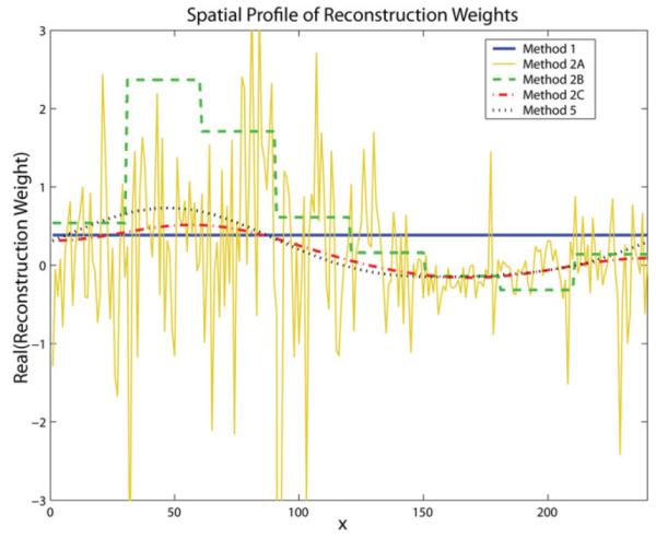
Representative reconstruction weights for the dataset in Fig. 2 are plotted vs. x-position for different CCDD methods. Method 1 weights exhibit no dependence on x (horizontal line), Method 2A weights fluctuate with each increment in x, Method 2B weights display a segmented dependence on x (Nseg = 8), whereas Method 2C and 5 weights exhibit smooth, low-frequency spatial variation over x. [Color figure can be viewed in the online issue, which is available at http://www.interscience.wiley.com.]
Reconstruction Efficiency Measurements
Generalized formulas estimating the number of complex-valued multiplications required for each phase of CCDD reconstruction were given in the Theory section and are summarized in Table 1. To provide a more intuitive sense of the magnitude of these values, numerical examples of computation expense are also reported, found by evaluating the generalized expressions using the following parameters: dx = 5, dy = 2, Nc = 8, Nx = 240, Ny = 240, Nu = 80, Nf = 20, Norder = 5, and R = 3. These numerical values are provided merely as examples; each imaging situation may require a different set of parameters that can alter the relative computational expense of these methods. Thus the generalized formulas should be consulted to predict the approximate computational cost for a particular set of parameters.
Table 1.
Approximate Number of Multiplications Required for CCDD Reconstruction*
| Calibration phase |
Weight conversion |
Synthesis phase |
||||
|---|---|---|---|---|---|---|
| Method | Generalized formula | Numerical example |
Generalized formula | Numerical example |
Generalized formula | Numerical example |
| 1 | NfNx(Ncdy)2 | 1,228,800 | – | – | dyNuNxNc2(R − 1) | 4,915,200 |
| 2A | >NfNx(Ncdy)2 | >1,228,800 | – | – | dyNuNxNc2(R − 1) | 4,915,200 |
| 2B | >NfNx(Ncdy)2 | >1,228,800 | – | – | dyNuNxNc2(R − 1) | 4,915,200 |
| 2C | >NfNx(NcdyNorder)2 | >30,720,000 | – | – | dyNuNxNc2(R − 1) | 4,915,200 |
| 3 | NfNx(Ncdxdy)2 | 30,720,000 | – | – | dxdyNuNxNc2(R − 1) | 24,576,000 |
| 4 | NfNx(Ncdxdy)2 | 30,720,000 | (logNx + logNy)NxNyNc2(R − 1) | 35,097,643 | NxNyNc2(R − 1) | 7,372,800 |
| 5 | NfNx(Ncdxdy)2 | 30,720,000 | (NxlogNx)dyNc2(R − 1) | 146,240 | dyNuNxNc2(R − 1) | 4,915,200 |
Approximate computational expense required to reconstruct coil-by-coil images using the five methods analyzed in this work, measured as the dominant number of complex-valued multiplications required for each phase of reconstruction. Generalized formulas expressed in terms of known acquisition and reconstruction parameters are reported, as well as example numerical values found by evaluating the formulas using the parameters used for the brain phantom in Fig. 2: dx = 5, dy = 2, Nc = 8, Nx = 240, Ny = 240, Nu = 80, Nf = 20, Norder = 5, R = 3.
It is clear from Table 1 that Method 1 has the most efficient calibration phase, requiring only NfNx(Ncdy)2 multiplications. As the dimensionality of the reconstruction model increases to account for 2D coil sensitivity variation, the computational expense increases significantly. For example, calculating smoothly varying hybrid-space reconstruction weights using Method 2C requires over NfNx(NcdxNorder)2 multiplications, a factor of at least Norder2 more than the same phase for Method 1. Although the computational expense of the calibration phase increases from Method 1 to Method 2C, the synthesis phase cost remains constant because in each case a 1D linear combination requiring dyNuNxNc2(R − 1) operations is performed, no matter whether the synthesis is performed in hybrid-space or k-space.
On the other hand, Methods 3–5 all share the same calibration phase expense to calculate 2D linear combination weights in k-space, requiring NfNx(Ncdxdy)2 multiplications each, but differ in their synthesis phase efficiency. Performing a 2D linear combination in k-space using Method 3 requires dxdyNuNxNc2 (R − 1) multiplications, or ~25 million operations in our example, whereas a 1D linear combination in hybrid-space using Method 5 requires only dyNuNxNc2 (R − 1) multiplications, or ~5 million operations—a computational savings factor of dx (the width of the 2D neighborhood along the kx-direction). Performing a point-by-point multiplication in image-space with Method 4 also offers computational savings over Method 3, requiring NxNyNc2 (R − 1) multiplications—a factor of dxdyNu/Ny fewer multiplications than synthesis in k-space. However, the computation required to convert the reconstruction weights from k-space into hybrid-space or image-space should also be considered for a complete assessment of computational burden. The weight conversion to image-space requires a considerable (logNx + logNy)NxNyNc2(R − 1) operations (assuming two FFTs are used). In our example, this conversion amounts to over 35 million extra multiplications—more than the cost of simply applying the weights in k-space. Though it is possible to achieve roughly a two-fold conversion efficiency improvement by interleaving the zero-padding and FFT operations, this conversion step still remains quite costly. On the other hand, the weight conversion to hybrid-space in Method 5 requires only (NxlogNx)dyNc2(R − 1) operations, or 146,240 operations in this example, a trivial expense by comparison.
The reconstruction accuracy results in Figs. 2 and 3 combined with the computational efficiency estimates in Table 1 emphasize an important trend observed in CCDD reconstruction: the better the image quality, the more computationally demanding the reconstruction. Methods 1, 2A, and 2B were relatively efficient but tended to be less accurate, whereas Methods 2C and 3–5 were less efficient but more accurate by comparison. The remainder of the analysis was thus focused on the latter group of methods in order to compare the relative efficiency of the most accurate reconstruction methods. According to our computational expense predictions, Method 3 was expected to be the least efficient method with its demanding calibration and synthesis phases, while Method 5 was expected to be most efficient due to its efficient weight conversion and synthesis. To validate the expected improvement in reconstruction speed of Method 5 over Method 3, actual measured reconstruction times for both methods were measured using the 124-slice phantom dataset. In Fig. 5a, the average reconstruction time per slice, including the calibration, weight conversion, and synthesis phases, is plotted as a function of dx for each method. As expected from theory, the reconstruction times for Methods 3 and 5 were convex functions of dx. For dx values greater than 1, Method 5 offered about a 40% reduction in total reconstruction time compared to Method 3.
FIG. 5.

a: Average measured computation time required to reconstruct a single-slice of a 124-slice dataset is plotted vs. dx, the neighborhood width in the kx-direction, using Methods 3 and 5. b: Measured reconstruction times to reconstruct the weight conversion (if applicable) and synthesis phase only. Dataset was acquired and reconstructed with the same parameters as the brain phantom in Fig. 2. [Color figure can be viewed in the online issue, which is available at http://www.interscience.wiley.com.]
To isolate the source of the computational efficiency improvement, the average time required to perform only the conversion and synthesis phase for each slice is plotted in Fig. 5b as a function of dx. In this case, the data for Method 3 was shown to perfectly fit a linear equation with a slope of 0.048 (with a small intercept value), indicating that the variable synthesis phase cost scaled proportionally with dx, as predicted in Table 1. On the other hand, the computation time for Method 5 remained fixed at 0.051 s per slice for all dx values because data synthesis was efficiently performed as a 1D linear combination in hybrid-space, eliminating the dependence on dx altogether. Using this data, the anticipated synthesis phase computational advantage of Method 5 over Method 3 was confirmed to be roughly dx in practice.
DISCUSSION
By treating CCDD reconstruction as two distinct phases and separately analyzing the computational expense of each phase, the most computationally intensive steps can easily be identified. This knowledge allows one to tailor the reconstruction pathway for a given application to exploit the computational advantages available in certain data domains. Fig. 6 presents a flowchart of various CCDD reconstruction methods described in this work, illustrating the possible processing pathways from accelerated input data to reconstructed output data. The data domains are indicated along the vertical direction and the reconstruction phases progress from left to right. All processing steps that are shared among all methods, such as the two 1D FTs required to convert k-space data to image-space data, are ignored in this figure; only steps imposing unique computational requirements are shown. The estimated computational expense for each step is indicated within each processing block, using the numerical examples from Table 1. The net reconstruction cost for a given pathway can be calculated by summing the expenses over all steps.
FIG. 6.
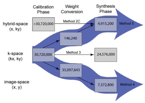
Flowchart illustrating various possible CCDD reconstruction pathways. Data domains are indicated vertically and reconstruction phases progress from left to right. The estimated computational expense for each step is indicated within each processing block, using the numerical examples from Table 1. The central horizontal pathway (Method 3) represents the conventional approach of performing the entire reconstruction in k-space. The reconstruction can also be performed entirely in hybrid-space, as indicated by the top horizontal pathway (Method 2C), which offers a more efficient synthesis phase than Method 3. The thick downward array illustrates “split-domain” Method 4, whereby calibration is performed in k-space and synthesis is performed efficiently image-space, with a costly weight conversion step in between. The other split-domain method, indicated by the thick upward arrow (Method 5), performs the calibration phase in k-space and the synthesis phase in hybrid-space, with a negligible weight conversion step in between. [Color figure can be viewed in the online issue, which is available at http://www.interscience.wiley.com.]
The central horizontal pathway in Fig. 6, labeled Method 3, represents the conventional, computationally intensive approach of performing the entire reconstruction in k-space. Alternatively, the reconstruction can be performed entirely in hybrid-space, as indicated by the top horizontal pathway labeled Method 2C, which requires a slightly more intensive calibration phase but offers a more efficient synthesis phase than Method 3. Another option is to use a split-domain approach. For example, the thick downward array illustrates the Method 4 pathway, whereby calibration is performed in k-space and synthesis is performed efficiently image-space, with a costly weight conversion step in between. For reconstruction of a single image, Method 4 may not be preferable over Method 3 due to the former method’s computationally demanding weight conversion step and uniform undersampling requirement. For reconstruction of multiple images in a time series, however, Method 4 becomes a more attractive option because ACS lines can be acquired once (or intermittently) during a scan and then applied to multiple subsequent images acquired with full acceleration. In that case, the computationally intensive conversion step would only need to be performed once (or only periodically), and the benefit of improved image-space synthesis efficiency could more fully be realized. Another consideration for Method 4 is its demanding memory allocation requirements: Nc2(R − 1) different weight images of size [Nx × Ny] must be stored and accessed during reconstruction, compared to the same number of smaller [dx × dy] k-space kernels required for Method 3. Although in this work we did not explicitly look at memory issues, it is worth noting that reconstruction pathways such as Method 4 may also impact memory requirements, especially as Nc and R increase.
The other split-domain method, indicated by the thick upward arrow in Fig. 6 labeled Method 5, performs the calibration phase in k-space and the synthesis phase in hybrid-space, with a negligible weight conversion step in between. Method 5 offers the most efficient reconstruction pathway for a majority of imaging applications by exploiting the computational efficiency afforded by the combination of k-space calibration and hybrid-space synthesis, while retaining the ability to reconstruct nonuniform sampling patterns, such as datasets with ACS lines included.
It should be clear that Fig. 6 is not an exhaustive list of all possible CCDD pathways but merely the most practical ones. For example, calibration and synthesis could conceivably both be performed in image-space; however, this would require the direct calculation of reconstruction weights for each image-space location, increasing the size of the matrix inversion problem to a prohibitively large size.
The flexibility of CCDD reconstruction to perform the calibration and synthesis phases in any data domain challenges the conventional wisdom that CCDD is exclusively a “k-space method.” CCDD reconstruction was shown to perform with equivalent accuracy in k-space (kx, ky), hybrid-space (x, ky), and image-space (x, y). Thus it is not that CCDD reconstruction is performed in a particular data space that distinguishes it from other methods but rather the data-driven nature of the CCDD reconstruction model itself. For instance, while Method 4 bears a resemblance to SENSE in that the unaliasing step is performed in image-space, the reconstructed image quality has been shown to vary significantly due to inherent calibration differences between physically-based and data-driven methods (27).
The results presented here demonstrate that reconstruction accuracy and efficiency varies considerably among CCDD reconstruction methods. Whereas the original 1D neighborhood k-space-based reconstruction (Method 1) was the most efficient method, it resulted in considerable residual aliasing for the configurations tested, presumably due to inadequate mathematical modeling of the underlying physical system. Calculating unique 1D neighborhood reconstruction weights at each x-location in hybrid-space (Method 2A) allowed for the possibility of weight variation over the x-direction, but poor system conditioning gave rise to noisy, low quality reconstructions. While reconstruction accuracy for Method 2A could be improved in practice by acquiring more ACS lines, this would reduce calibration phase efficiency as well as net acceleration. Expanding Method 2 to segmented calibration (Method 2B) improved image quality considerably without impacting net acceleration; however, there remained the possibility of signal discontinuities at the junctions between segments. These discontinuities could potentially be avoided by using an overlapping segment approach followed by interpolation (19), although this approach was not tested in this work.
Smoothly varying hybrid-space calibration (Method 2C) related the weights along x to one another in a continuous manner, offering improved image quality but slightly increased calibration complexity. While only one type of basis function was employed here, Method 2C may offer additional benefits because the choice of basis function can be flexibly adjusted to satisfy a particular parameter or configuration. Methods 3–5 produced the highest image quality by extending the reconstruction model to include a second dimension of coil sensitivity while still being highly overdetermined. Among Methods 3–5, Method 5 was shown to have the least computational cost due to its efficient application of weights in hybrid-space during data synthesis.
While split-domain methods such as Method 5 improve synthesis phase efficiency, the calibration phase cost to calculate 2D k-space neighborhood weights can represent a disproportionately large part of total reconstruction cost, resulting in diminished net computational benefit. This scenario highlights the need for techniques to alleviate the calibration phase burden to further speed up overall reconstruction. Recently, Beatty et al. (28) have demonstrated a new implementation for improving calibration phase efficiency that can be incorporated with split-domain methods for added gains in net reconstruction speed.
This work investigated five basic categories of CCDD methods; however, due to space considerations, some variations proposed in the literature were omitted. For example, non-shift-invariant k-space-based reconstructions that segment the reconstruction along kx (25) or kx and ky (29) have been demonstrated. For these and other cases, the qualitative imaging results and computational expense predictions reported above may be extrapolated to provide a general assessment of reconstruction accuracy and efficiency.
In Table 1, CCDD reconstruction cost was shown to grow proportionally with several imaging and system parameters, including image size, reduction factor, and the square of the number of coils. These relationships should help predict how computational complexity would scale as these parameters are varied. In particular, the squared computational dependence on the number of coils will become an increasingly important consideration with the availability of high-channel systems capable of supporting greater number of coils and higher accelerations.
CONCLUSIONS
This work compared various CCDD methods in order to identify their relative merits for a given imaging application. We showed that by treating the calibration and synthesis phases as discrete steps in the CCDD reconstruction, each step could be independently optimized for accuracy and/or efficiency. The choice of data domain in which each step occurs can be flexibly tailored to a given application, enabling split-domain approaches such as Methods 4 and 5. Method 5 was shown to combine the accuracy of a 2D k-space neighborhood calibration with the efficiency of a 1D neighborhood reconstruction in hybrid-space, offering image quality and computational advantages over previous techniques. This evaluation of the accuracy and efficiency tradeoffs associated with various CCDD reconstruction pathways may help guide the selection of appropriate PI reconstruction methods for a particular imaging task.
Footnotes
This measure is akin to the “big O” notation used in computer science to describe the asymptotic upper bound of algorithmic complexity.
REFERENCES
- 1.Pruessmann KP, Weiger M, Scheidegger MB, Boesiger P. SENSE: sensitivity encoding for fast MRI. Magn Reson Med. 1999;42:952–962. [PubMed] [Google Scholar]
- 2.Wang J, Kluge T, Nittka M, Jellus V, Kuehn B, Kiefer B. 1st Workshop on Parallel MRI: Basics and Clinical Applications. Würzberg, Germany: 2001. Parallel acquisition techniques with modified SENSE reconstruction (mSENSE) p. 92. [Google Scholar]
- 3.Sodickson DK, McKenzie C. A generalized approach to parallel magnetic resonance imaging. Med Phys. 2001;28:1629–1643. doi: 10.1118/1.1386778. [DOI] [PubMed] [Google Scholar]
- 4.Kyriakos W, Panych L, Kacher D, Westin C, Bao S, Mulkern R, Jolesz F. Sensitivity profiles from an array of coils for encoding and reconstruction in parallel (SPACE RIP) Magn Reson Med. 2000;44:301–308. doi: 10.1002/1522-2594(200008)44:2<301::aid-mrm18>3.0.co;2-d. [DOI] [PubMed] [Google Scholar]
- 5.Griswold MA, Jakob PM, Nittka M, Goldfarb J, Haase A. Partially parallel imaging with localized sensitivities. Magn Reson Med. 2000;44:602–609. doi: 10.1002/1522-2594(200010)44:4<602::aid-mrm14>3.0.co;2-5. [DOI] [PubMed] [Google Scholar]
- 6.Pruessmann KP, Weiger M, Bornert P, Boesiger P. Advances in sensitivity encoding with arbitrary k-space trajectories. Magn Reson Med. 2001;46:638–651. doi: 10.1002/mrm.1241. [DOI] [PubMed] [Google Scholar]
- 7.Griswold MA, Kannengiesser S, Heidemann RM, Wang J, Jakob PM. Field-of-view limitations in parallel imaging. Magn Reson Med. 2004;52:1118–1126. doi: 10.1002/mrm.20249. [DOI] [PubMed] [Google Scholar]
- 8.Goldfarb J. The SENSE ghost: field-of-view restrictions for SENSE imaging. J Magn Reson Imaging. 2004;20:1046–1051. doi: 10.1002/jmri.20204. [DOI] [PubMed] [Google Scholar]
- 9.Jakob PM, Griswold MA, Edelman RR, Sodickson DK. AUTO-SMASH, a self-calibrating technique for SMASH imaging. MAGMA. 1998;7:42–54. doi: 10.1007/BF02592256. [DOI] [PubMed] [Google Scholar]
- 10.Heidemann RM, Griswold MA, Haase A, Jakob PM. VD-AUTO-SMASH imaging. Magn Reson Med. 2001;45:1066–1074. doi: 10.1002/mrm.1141. [DOI] [PubMed] [Google Scholar]
- 11.Griswold MA, Jakob PM, Heidemann RM, Nittka M, Jellus V, Wang J, Kiefer B, Haase A. Generalized autocalibrating partially parallel acquisitions (GRAPPA) Magn Reson Med. 2002;47:1202–1210. doi: 10.1002/mrm.10171. [DOI] [PubMed] [Google Scholar]
- 12.Kholmovski EG, Samsonov AA. GARSE: generalized autocalibrating reconstruction for sensitivity encoded MRI; Proceedings of the 13th Annual Meeting of ISMRM; Miami Beach, FL, USA. 2005; (Abstract 2672) [Google Scholar]
- 13.Wang Z, Wang J, Detre JA. Improved data reconstruction method for GRAPPA. Magn Reson Med. 2005;54:738–742. doi: 10.1002/mrm.20601. [DOI] [PubMed] [Google Scholar]
- 14.Skare S, Bammer R. Spatial modeling of the GRAPPA weights; Proceedings of the 13th Annual Meeting of ISMRM; Miami Beach, FL, USA. 2005; (Abstract 2422) [Google Scholar]
- 15.Griswold MA, Breuer F, Blaimer M, Kannengiesser S, Heidemann RM, Mueller M, Nittka M, Jellus V, Kiefer B, Jakob PM. Autocalibrated coil sensitivity estimation for parallel imaging. NMR Biomed. 2006;19:316–324. doi: 10.1002/nbm.1048. [DOI] [PubMed] [Google Scholar]
- 16.Blaimer M, Breuer F, Mueller M, Seiberlich N, Ebel D, Heidemann RM, Griswold MA, Jakob PM. 2D-GRAPPA-operator for faster 3D parallel MRI. Magn Reson Med. 2006;56:1359–1364. doi: 10.1002/mrm.21071. [DOI] [PubMed] [Google Scholar]
- 17.Blaimer M, Breuer F, Mueller M, Heidemann R, Griswold M, Jakob P. SMASH, SENSE, PILS, GRAPPA: how to choose the optimal method. Top Magn Reson Imaging. 2004;15:223–236. doi: 10.1097/01.rmr.0000136558.09801.dd. [DOI] [PubMed] [Google Scholar]
- 18.Wang J, Zhang B, Zhong K, Zhuo Y. Image domain based fast GRAPPA reconstruction and relative SNR degradation; Proceedings of the 13th Annual Meeting of ISMRM; Miami Beach, FL, USA. 2005. (Abstract 2428) [Google Scholar]
- 19.Kholmovski EG, Parker DL. Spatially variant GRAPPA; Proceedings of the 14th Annual Meeting of ISMRM; Seattle, WA, USA. 2006. (Abstract 285) [Google Scholar]
- 20.Griswold MA. Second International Workshop on Parallel MRI. Zurich, Switzerland: 2004. Advanced k-space techniques; pp. 16–18. [Google Scholar]
- 21.Qu P, Wu B, Wang C, Shen GX. Optimal utilization of acquired k-space points for GRAPPA reconstruction; Proceedings of the 13th Annual Meeting of ISMRM; Miami Beach, FL. 2005. (Abstract 2667) [DOI] [PubMed] [Google Scholar]
- 22.Bankson J, Wright S. Generalized partially parallel imaging with spatial filters; Proceedings of the 9th Annual Meeting of ISMRM; Honolulu, HI, USA. 2001. (Abstract 1795) [Google Scholar]
- 23.Bracewell R. Two-dimensional imaging. Prentice-Hall, Inc; Englewood Cliffs, NJ: 1995. [Google Scholar]
- 24.Brau AC, Beatty PJ, Skare S, Bammer R. Efficient computation of autocalibrating parallel imaging reconstructions; Proceedings of the 14th Annual Meeting of ISMRM; Seattle, WA, USA. 2006. (Abstract 2462) [Google Scholar]
- 25.Park J, Zhang Q, Jellus V, Simonetti O, Li D. Artifact and noise suppression in GRAPPA imaging using improved k-space coil calibration and variable density sampling. Magn Reson Med. 2005;53:186–193. doi: 10.1002/mrm.20328. [DOI] [PubMed] [Google Scholar]
- 26.Wang Z, Fernandez-Seara M. 2D partially parallel imaging with k-space surrounding neighbors-based data reconstruction. Magn Reson Med. 2006;56:1389–1396. doi: 10.1002/mrm.21078. [DOI] [PubMed] [Google Scholar]
- 27.Beatty PJ, Brau AC. Understanding the GRAPPA paradox; Proceedings of the 14th Annual Meeting of ISMRM; Seattle, WA, USA. 2006. (Abstract 246) [Google Scholar]
- 28.Beatty P, Brau A, Chang S, Joshi S, Michelich C, Bayram E, Nelson T, Herfkens R, Brittain J. A method for autocalibrating 2D-accelerated volumetric parallel imaging with clinically practical reconstruction times; Proceedings of the Joint Annual Meeting ISMRM-ESMRMB; Berlin, Germany. 2007. p. 1749. [Google Scholar]
- 29.Guo J-Y, Kholmovski EG, Zhang L, Jeong E-K, Parker DL. k-Space inherited parallel acquisition (KIPA): application on dynamic magnetic resonance imaging thermometry. Magn Reson Imaging. 2006;24:903–915. doi: 10.1016/j.mri.2006.03.001. [DOI] [PubMed] [Google Scholar]