Identifying systematic errors in quantitative dynamic-susceptibility contrast perfusion imaging by high-resolution multi-echo parallel EPI

Abstract

Several obstacles usually confound a straightforward perfusion analysis using dynamic-susceptibility contrast-based magnetic resonance imaging (DSC-MRI). In this work, it became possible to eliminate some of these sources of error by combining a multiple gradient-echo technique with parallel imaging (PI): first, the large dynamic range of tracer concentrations could be covered satisfactorily with multiple echo times (TE) which would otherwise result in overestimation of image magnitude in the presence of noise. Second, any bias from T₁ relaxation could be avoided by fitting to the signal magnitude of multiple TEs. Finally, with PI, a good tradeoff can be achieved between number of echoes, brain coverage, temporal resolution and spatial resolution. The latter reduces partial voluming, which could distort calculation of the arterial input function. Having ruled out these sources of error, a 4-fold overestimation of cerebral blood volume and flow remained, which was most likely due to the completely different relaxation mechanisms that are effective in arterial voxels compared with tissue. Hence, the uniform tissue-independent linear dependency of relaxation rate upon tracer concentration, which is usually assumed, must be questioned. Therefore, DSC-MRI requires knowledge of the exact dependency of transverse relaxation rate upon tracer concentration in order to calculate truly quantitative perfusion maps.

INTRODUCTION

Dynamic-susceptibility contrast-based magnetic resonance imaging (DSC-MRI) is an evolving technology for studying cerebral hemodynamics and blood flow. Thereby, $T_2^{\ast }$-weighted time series are acquired during the first pass of an intravascular tracer. It is commonly assumed that the resulting increase in relaxation rate, $\mathrm{\Delta }{R}_2^{\ast }$, is proportional to the tracer concentration. From these dynamic scans, it is then possible to estimate cerebral blood volume (CBV) in tissue by normalizing the integral of the concentration time course using that of an arterial voxel (with a known CBV) as a reference. Furthermore, pixel-wise deconvolution with an arterial input function (AIF) yields the tissue residue function, from which maps of mean transit time (MTT) and cerebral blood flow (CBF) can be calculated (1, 2).

Although DSC-MRI is a powerful technique for detection of abnormal perfusion, for example in acute cerebral ischemia, it remains unclear whether truly quantitative CBV/CBF analysis is possible with conventional techniques. This is because the following obstacles usually confound a straightforward quantitative CBV/CBF analysis:

1. Because CBV is normalized by the integral over the AIF, partial voluming in AIF voxels can lead to erroneous CBV and CBF. A correction scheme was proposed in (3, 4) based on fitting the complex signal to a spiral-like curve in the complex plane in order to eliminate the static offset arising from partial tissue volume. However, due to the periodic nature of the spiral, false minima exist which make the method less robust in the presence of noise. Furthermore, this scheme is only valid for arteries parallel to B₀, i.e. if the extravascular field and, hence, the signal around the vessel is left unaltered by the contrast agent.

2. It can be expected that the uniform (i.e. tissue-independent) linearity between $\mathrm{\Delta }{R}_2^{\ast }$ and tracer concentration, which is usually assumed, does not hold true for the large dynamic range of concentrations encountered in a DSC-MRI experiment. In particular, when comparing arterial voxels (containing bulk blood) with a tissue voxel (with a vascular network), the uniform linearity is questionable (5, 6). This is because completely different contrast mechanisms are effective: relaxation in bulk blood is due to molecular interactions and dynamic dephasing, i.e. water diffusion and/or exchange in the presence of field gradients and/or frequency shifts generated by compartments which contain the contrast agent. On the other hand, the mostly extravascular relaxation in tissue voxels is mainly due to static intra-voxel dephasing in the vicinity of blood vessels.

3. The dynamic range of the observable MR signal can be too small for high tracer concentrations in arterial voxels if an echo time (TE) of the order of 50–60 ms is used. Hence, the AIF amplitude is biased by the noise floor of MR magnitude data and is therefore underestimated. This leads to an overestimation of CBV and CBF.

4. Since the tracer not only decreases $T_2^{\ast }$, but also T₁, which has the opposite effect on signal intensity, the tracer concentration may be underestimated by a certain factor. As this factor generally depends nonlinearly on the tracer concentration, it is different in AIF and tissue voxels and therefore distorts CBV and CBF calculations.

5. An additional delay and dispersion during transport of the bolus from the site of AIF calculation (major arterial vessel) to the tissue voxel under observation can confound the residue function and could be falsely attributed to the voxel itself. Thus, this delay/dispersion introduces errors in MTT/CBF calculations.

To investigate which of these obstacles is most important, we used a multi-echo (ME) approach for gradient-echo based DSC-MRI (1,7–9) because it helps tackle items (C) and (D): First, if the signal magnitude of late echoes drops below detectability, i.e. the magnitude is equal to or less than the noise amplitude, the erroneous influence of these echoes on the calculated $\mathrm{\Delta }{R}_2^{\ast }$ can be suppressed using only the first echo (9), for example by a magnitude-weighted exponential fit. In other words, because the contrast-to-noise ratio is optimal at $TE\approx T_2^{\ast }$, ME provides an extended range of optimal sensitivity over a wider range of $T_2^{\ast }$ values in the presence of strong $T_2^{\ast }$ variations. Second, because $\mathrm{\Delta }{R}_2^{\ast }$ can be calculated by fitting to the signal magnitude as a function of TE, it is undisturbed from T₁ enhancement caused by the tracer, which is the same for all TEs. This is particularly advisable if the blood–brain barrier is disrupted, in which case significant T₁ relaxation can be expected in tissue.

In order to acquire multiple gradient echoes after a single excitation with high spatial resolution, parallel imaging (PI) can be employed for DSC-MRI (10) to shorten the EPI readouts. In addition, using PI has two advantages: First, image artifacts related to EPI are reduced by the increased bandwidth per pixel in phase encoding direction. This also reduces the spatial shift of arterial voxels during bolus passage which is observed due to the transient changes in magnetic susceptibility in the blood plasma. Second, partial-volume effects are decreased because of the spatial resolution enhancement achievable by PI, i.e. it helps circumvent item (A). We will refer to this technique, i.e. the combination of ME with PI, as perfusion with multiple echoes and temporal enhancement (PERMEATE).

Additionally, we will address the question whether the combination of ME with PI provides a significant gain in the accuracy of determining tracer concentration in comparison with those derived from single-echo techniques (optionally with PI). This accuracy is a prerequisite for quantitative CBV/CBF measurements. With data available from ME at different TEs, we had the opportunity to develop an optimal strategy to select arterial voxels for automatic AIF calculation (11,12). Furthermore, calculation of the AIF and tissue time course with respect to the underlying contrast-material concentration could be improved by ME. Also, it will be estimated whether or not there is a benefit in signal-to-noise ratio (SNR) from using ME over single-echo data when combined with PI. Finally, based on our results, we would like to answer the question whether truly quantitative DSC-MRI is possible with conventional single-shot EPI techniques and/or PERMEATE.

EXPERIMENTAL

In this section, the experimental setup will be described, and an optimal technique to calculate the AIF will be developed based on the ME data. In addition, different strategies will be presented to calculate concentration time courses from gray and white matter from the ME data. Finally, formulae will be given to estimate the gain in SNR of PERMEATE over single-echo techniques.

Experimental setup

All scans were performed on a 1.5 T scanner (Signa LX/i, GE Medical Systems, Waukesha, WI, USA) fitted with high performance gradients (maximum strength, 50 mT/m; rise time, 270 μs). PI was performed by means of an eight-element brain coil (MR Devices, Waukesha, WI, USA) and two different reduction factors: R = 3 and R = 4. A multi-echo multi-slice gradient-echo EPI sequence (13) was used to image 15 slices (5 mm thickness, 1 mm gap) with 240 mm FOV and an acquisition matrix size of 96 × 96. In our experiments, the number of echoes equaled the reduction factor. Sequence parameters were: TE = 13.8, 31.6 and 49.4 ms (R = 3) and TE = 12.4, 27.3, 42.2 and 57.1 ms (R = 4), 100 repetitions with TR = 1225 ms, ±100 kHz receiver bandwidth and a flip angle of 70°. To reach a steady state, data acquisition was preceded by six (R = 3) or eight (R = 4) dummy cycles. A single dose of 0.1 mmol/kg Gd-DTPA was administered at a rate of 4 ml/s followed by a 20 ml saline flush into the arm vein using a power injector. The technique was tested with 32 and 50-year-old healthy subjects with R = 3, 4 and R = 4, respectively. Image reconstruction was performed using a GRAPPA-based algorithm (14). To account for the differing acquisition time of different slices within one TR, image magnitudes were interpolated to the same point in time.

AIF selection

A completely automated selection of AIF (11) was used to avoid any bias from human interaction. The procedure and selection criteria of voxels contributing to the AIF were similar to those in (12): a Gaussian fit was applied to the time course of each voxel. The parameters of the Gaussian function, i.e. amplitude A, width τ and time offset t₀ were normalized by subtracting the mean value of all brain voxels and dividing by the standard deviation: x′ = (x − x̄)/〈x〉 with x = {A, τ, t₀}. The normalization makes the selection independent of scaling and shifting of values which may vary from scan to scan. The general criterion for an AIF voxel is a large A′, a small τ′ and an early $t_0^{\prime }$. Thus, all voxels with A′ <0, τ′>0 and $t_0^{\prime }>0$ were excluded and a score $A^{\prime }·(-t_0^{\prime })·(-{\tau }^{\prime })$ was assigned to each remaining voxel. The N voxels with the highest score were selected. Finally, isolated voxels, i.e. those voxels without any selected voxels as their next neighbors, were removed from the cluster to avoid bias from voxels included accidentally because of noise-based shape resembling a sharp bolus.

Using the above algorithm, there are several factors that can have an impact on the cluster of selected voxels, the AIF derived from these voxels, and hence on the CBV and CBF maps:

• The AIF can be derived separately from each echo and from an exponential fit, realized in the following by a linear regression of the logarithm of the magnitude as a function of TE. In the latter, the error σ, which was used in the fit to estimate the uncertainty of each data point (15), was set to σ = m^−w for magnitude m at a certain TE with w = 0, 1, 2.

• Averaging over a large number of arterial voxels stabilizes the AIF, but introduces more and more partial voluming as voxels with smaller arterial contribution or more distant from large arteries are incorporated. Thus, the dependency of the AIF upon N was studied with N = 10, 20, 40 and 80 to test whether the choice of N has a significant impact on the shape of the AIF.

• Slight in-plane smoothing is usually used to reduce noise, but can also affect the AIF due to non-arterial contributions coming from adjacent voxels. hence, the AIF was calculated as a function of smoothing with a Gaussian kernel with full-width-at-half-maximum (FWHM) of 0, 1 and 2 pixels.

To investigate the degree to which the shape of the AIF depends on the aforementioned parameters, different AIF were calculated from the data of the 32-year-old healthy subject (R = 4) by varying these parameters. After calculating the time course of each voxel with different settings, the algorithm to select AIF voxels was based on this differing data. An AIF was considered optimal if it had a high, early and sharp peak and minimal corruption by T₁ relaxation or noise.

CBV and CBF in gray/white matter

To estimate the benefit of using ME in comparison to a conventional single echo approach for CBV and CBF calculations, gray matter (GM) and white matter (WM) regions were selected manually in the frontal cortex and white matter (superior corona radiata), serving as masks for further calculations. The $\mathrm{\Delta }{R}_2^{\ast }$ time course resulting from each echo and the weighted fit was evaluated separately for each tissue type. Maps of CBV were generated according to (1), i.e. dividing the integrated time course by the integral over the AIF and correction for differences in hematocrit between large and small vessels. Pixel-wise calculation of the residue function, which finally yielded MTT and CBF, was performed by block-circulant singular-value decomposition for tracer arrival timing-insensitive deconvolution (16) with a tolerance threshold P_SVD = 10%. This block-circulant deconvolution prevents errors due to differences in bolus-arrival time between the feeding artery and the voxel in question, item (E).

SNR evaluations

Parallel imaging studies are normally penalized by an SNR loss of factor g√R over conventional studies, where g is the geometry factor of the coil used for PI. On the other hand, PI reduces EPI-related susceptibility artifacts. Thus, it is desirable to use it for functional studies, especially for DSC-MRI. In addition, by increasing the reduction factor and thereby decreasing the readout duration, it becomes possible to acquire multiple echoes, where, without PI, only a single echo could be acquired.

To estimate theoretically whether PERMEATE yields a gain or loss in SNR when calculating $\mathrm{\Delta }{R}_2^{\ast }$ in comparison to using single-echo PI or non-PI imaging, noise propagation was analyzed. The fluctuation σ_m of the signal magnitude m at different TEs is assumed to be independent of TE. This assumption is justified if σ_m can be considered as infinitesimally small, which in turn is a prerequisite for analyzing error propagation. Thus, it can be expressed relative to m₀, the signal magnitude at TE = 0: σ_m = ε · g√R with a dimensionless noise factor ε unique to each voxel. The factor g√R deviates from one if parallel imaging is employed.

Single echo

Assuming a single exponential decay, the signal magnitude is given by

$$m=m_0·exp(-[R_{2,0}^{\ast }+\mathrm{\Delta }{R}_2^{\ast }]TE)$$ (1)

with $R_{2,0}^{\ast }$ as the native tissue/blood relaxation rate without contrast agent. $\mathrm{\Delta }{R}_2^{\ast }$ from a single echo at TE is then obtained by

$$\mathrm{\Delta }{R}_2^{\ast }=-\frac{log(m)}{TE}+\frac{log(m_0)}{TE}-R_{2,0}^{\ast }$$ (2)

The term

$$\frac{log(m_0)}{TE}-R_{2.0}^{\ast }$$

in the above equation is usually calculated by averaging over pre-bolus values (with $\mathrm{\Delta }{R}_2^{\ast }=0$). It is assumed that a sufficiently large number of pre-bolus values are available so that fluctuations of this term can be neglected. Analysis of error propagation, i.e. how sample noise affects the precision of estimating $\mathrm{\Delta }{R}_2^{\ast }$, reveals that the noise of $\mathrm{\Delta }{R}_2^{\ast }$ is given by

$$\begin{array}{l}{\sigma }_{\mathrm{\Delta }{R}_2^{\ast }}^{\text{single}}=\left|\frac{\partial \mathrm{\Delta }{R}_2^{\ast }}{\partial m}\right|{\sigma }_m\\ =g\sqrt{R_{\text{single}}}\frac{\epsilon }{TE}exp([R_{2,0}^{\ast }+\mathrm{\Delta }{R}_2^{\ast }]TE)\end{array}$$ (3)

Multi-echo

If multiple signal magnitudes, m_i, at different echo times, TE_i, are measured, linear regression of

$$y_i=log(m_i)=log(m_0)-[R_{2,0}^{\ast }+\mathrm{\Delta }{R}_2^{\ast }]{TE}_i$$ (4)

yields the term in brackets. Further subtraction of $R_{2,0}^{\ast }$, averaged over pre-bolus results (and therefore considered noise-free), yields $\mathrm{\Delta }{R}_2^{\ast }$. The error σ_i of each y_i is given by

$${\sigma }_i=\left|\frac{\partial y_i}{\partial m_i}\right|{\sigma }_m=\epsilon ·s_i=\epsilon ·exp([R_{2,0}^{\ast }+\mathrm{\Delta }{R}_2^{\ast }]{TE}_i)$$ (5)

By using formulae in (15) to calculate the error propagation of linear regression, the noise of $\mathrm{\Delta }{R}_2^{\ast }$ is then

$${\sigma }_{\mathrm{\Delta }{R}_2^{\ast }}^{\text{multi}}=g\sqrt{R_{\text{multi}}}·\epsilon ·\sqrt{\frac{{\mathrm{\sum }}_{i}1/s_i^2}{({\mathrm{\sum }}_{i}1/s_i^2){\mathrm{\sum }}_i{TE}_i^2/s_i^2)-{({\mathrm{\sum }}_i{TE}_i/s_i^2)}^2}}$$ (6)

In conclusion, the ratio ${\sigma }_{\mathrm{\Delta }{R}_2^{\ast }}^{\text{single}}/{\sigma }_{\mathrm{\Delta }{R}_2^{\ast }}^{\text{multi}}$ is independent of ε and also independent of g√R if the same PI reduction is used, i.e. if R_single = R_multi. It is equivalent to the ratio of SNRs, SNR_multi/SNR_single, because the determined $\mathrm{\Delta }{R}_2^{\ast }$, the ‘signal’, is the same. The ratio yields the gain (or loss) in SNR of PERMEATE in comparison to simple single-echo PI or non-PI imaging.

RESULTS

AIF selection

In Fig. 1(a), the AIF is shown for different echoes from the same experiment. Apparently, the AIF from the echo with the shortest TE provides the AIF with highest amplitude and a shape that resembles a single sharp bolus most closely. This TE dependency can be explained by three effects: first, different TEs have different dynamic ranges and the signal magnitude bounces off the noise floor which leads to underestimation of tracer concentration for long TEs. Second, looking at the location of voxels which were automatically selected for AIF calculation revealed that those from the shortest TE are exclusively in the internal carotid arteries (ICA). Because the ICA is located adjacent to air cavities, the signal from later echoes in these voxels is strongly attenuated due to intra-voxel dephasing so that the algorithm chooses voxels which are further downstream for longer TEs (but still in the ICA). This may cause increased partial voluming and, hence, underestimation of tracer concentration. Third, if $T_2^{\ast }$ is different for the the intra- and extravascular compartment, partial voluming becomes TE-dependent, which could also explain the different shapes of the curves. Since CBV is normalized by the integral over the AIF, the decreased integral in Fig. 1(a) for longer TEs leads directly to an overestimation of CBV and, hence, CBF. Please note that the integral of the first echo is slightly less than that of the second echo because of post-bolus T₁ relaxation. Below, a strategy will be presented to circumvent this source of error.

Figure 1.

(a) AIF calculated from different echoes. The AIF averaged over the time course of ~30 automatically selected voxels. The FWHM of in-plane smoothing was 1.0. Please note that, owing to the differing input to the automatic selection of AIF voxels, different clusters of voxels were used for AIF calculation. The integral over each time course is given by Σ in arbitrary units. (b) AIF calculated from weighted fit with different error-weighting exponents w (see text). Other parameters were the same as in (a). (c) AIF calculated from the maximum of the AIF from the first echo and the weighted fit with w = 1. Please note that the actual values of the combined AIF are slightly different from those of the constituent curves because there is a minor variation of the locations of automatically selected voxels. (d) Influence of the number of AIF voxels on the shape of the AIF. Note that the actual number of voxels is less than N (which is specified in brackets) because of the next-neighbor analysis as described in the text. The integral over each time course is given by Σ in arbitrary units. (e) The effect of in-plane smoothing with a Gaussian kernel of different width on the shape of the AIF. Data is from 33 automatically selected voxels

Another observation is the negative $\mathrm{\Delta }{R}_2^{\ast }$ in the post-bolus range of the first echo in Fig. 1(a). It is a consequence of decreased T₁, which leads to increased signal intensity compared to pre-bolus values, that in turn computes to negative $\mathrm{\Delta }{R}_2^{\ast }$ if only a single echo is used [equation (2)].

Calculating $\mathrm{\Delta }{R}_2^{\ast }$ by a weighted fit with exponent w is shown in Fig. 1(b). Here, the non-zero weighting puts more emphasis on earlier, high signal echoes. The fit with w = 1 appears most practical as it provides higher amplitude during bolus passage in comparison to w = 0, which is an unweighted fit, and fewer fluctuations compared with w = 2, which has wildly varying values as a consequence of decreased data basis of the fit. However, due to the reduced dynamic range of the later echoes, the calculated $\mathrm{\Delta }{R}_2^{\ast }$ is only half of that calculated from the first echo. In addition, due to the fit, the post-bolus range is undisturbed by T₁ relaxation.

Taking into account these intermediate results, a simple, yet effective, strategy will be used in further calculations to ensure a possibly high AIF amplitude, which is desirable during and after bolus passage: a time course is calculated for each voxel which consists of the maximum of the first-echo and from a weighted fit (w = 1) at each point in time. Automatic selection of AIF voxels is then performed using these curves. The result of this strategy is shown in Fig. 1(c).

The result of varying the number of (potential) AIF voxels, N, is shown in Fig. 1(d). The curves are almost similar, although that with N = 10 has an earlier onset than those with more voxels. By looking at the location of the voxels selected (data not shown), it becomes apparent that, the more voxels are selected, the further they are downstream in the ICA. As vessel size decreases with downstream position, partial voluming could becomes more likely. However, because the integrals under the curves are almost identical, apparently no severe partial voluming was introduced by increasing N. Thus, as a trade-off, N = 40 was used in further calculations.

According to Fig. 1(e), the width of the Gaussian kernel used for in-plane denoising can modify the AIF due to increased (artificial) partial voluming if it is larger than 1 pixel. Therefore, FWHM = 1 was chosen as a trade-off between retaining spatial resolution and reducing noise in all further evaluations.

CBV and CBF in gray/white matter

The $\mathrm{\Delta }{R}_2^{\ast }$ time course for GM and WM during bolus passage, evaluated either from the last echo or from a weighted fit, is shown in Fig. 2(a). The curve pairs for each tissue type are similar, indicating that the tracer concentration is low enough to avoid a significant dynamic range overshoot at TE = 57.1 ms. This is in contrast to the strong variations encountered in the curves of arterial voxels [Fig. 1(a) and (b)], where significant saturation was apparent. From Fig. 2(a), it is also obvious that the post-bolus $\mathrm{\Delta }{R}_2^{\ast }$ of the weighted fit in GM is higher than $\mathrm{\Delta }{R}_2^{\ast }$ obtained from a single echo. This difference can be explained by signal enhancement due to decreased T₁ in GM. The faster relaxation leads to an underestimation of tracer concentration if only a single echo is used. This is because $\mathrm{\Delta }{R}_2^{\ast }$ is calculated using the pre-bolus signal as a reference, which is not increased by T₁ relaxation. Of course, this reference is not required if a multi-echo fit is used. Thus, the $\mathrm{\Delta }{R}_2^{\ast }$ time course of ME is undisturbed by T₁ relaxation and reflects only $T_2^{\ast }$ relaxation. This issue becomes increasingly relevant with decreasing TR. The effect is less pronounced in WM because of less CBV.

Figure 2.

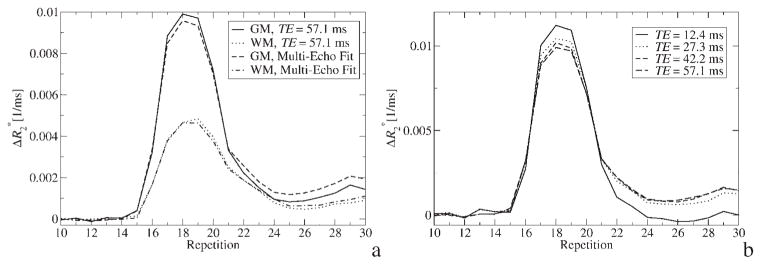
(a) $\mathrm{\Delta }{R}_2^{\ast }$ time course within GM and WM regions for the last echo with TE ms = 57.1 and for a weighted fit with w = 1. (b) $\mathrm{\Delta }{R}_2^{\ast }$ time course within GM regions for different TEs

Figure 2(b) depicts $\mathrm{\Delta }{R}_2^{\ast }$ curves in GM calculated from different echoes. Two observations can made: first, as in AIF voxels [Fig. 1(a)], dynamic range differences during the first pass of the bolus lead to different time courses for different TEs. However, the effect is less prominent than in AIF voxels since the tracer concentration is lower. Second, since there is residual plasma concentration after the first pass of the tracer, a calculated $\mathrm{\Delta }{R}_2^{\ast }$ of approximately zero in the post-bolus interval of TE = 12.4 ms indicates that the effects of $T_2^{\ast }$ and T₁ relaxation on the signal cancel each other. Thus, the time course of the echo with the shortest TE is heavily biased by T₁ relaxation. For later echoes, the $T_2^{\ast }$ effect outweighs T₁ relaxation.

Quantitative CBV (Fig. 3) and CBF (Fig. 4) maps are shown for the weighted fit with w = 1 and for the last echo, respectively. Although, the maps generated from the weighted fit are slightly less susceptible to intra-voxel dephasing by large-scale field inhomogeneities (as seen in the lower slices) because of the incorporation of data from early echoes, the maps are visually almost similar. However, quantitatively, CBV (and consequently CBF) values differ significantly (Table 1): the CBV values derived from the last echo are underestimated due to decreased T₁.

Figure 3.

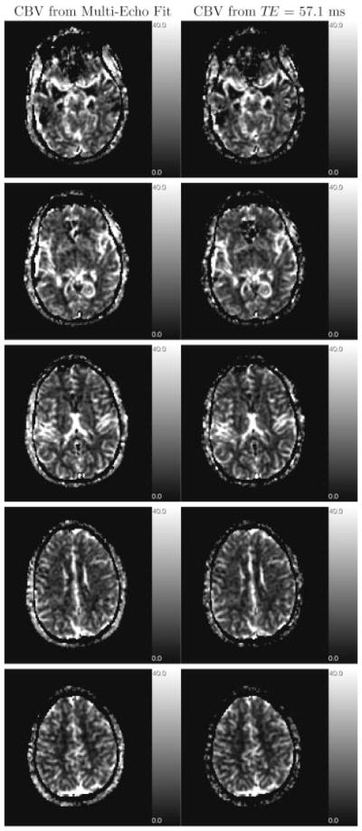
CBV maps, generated from weighted fit (left column), and from echo with TE = 57.1 ms (right column) of every other slice. Gray-scale coded values are in ml/100 g

Figure 4.

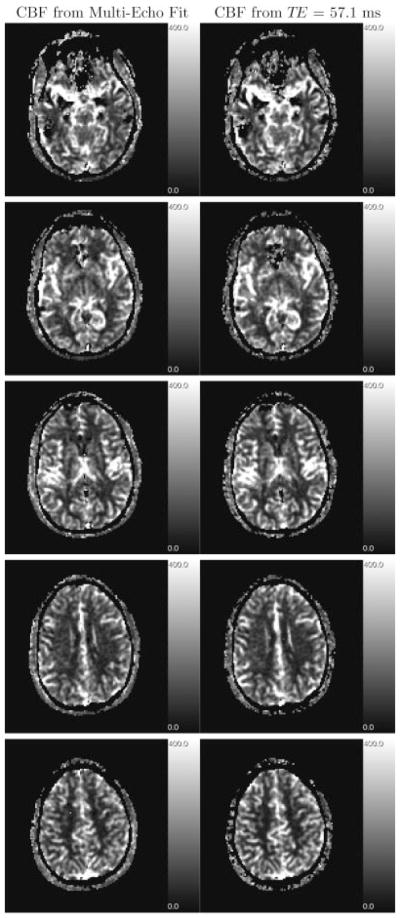
CBF maps, generated from weighted fit (left column), and from echo with TE = 57.1 ms (right column) of the same slices as in Fig. 3. Deconvolution was performed using an AIF calculated by the maximum method as described in the text. Gray-scale coded values are in ml/100 g/min

Table 1.

Measured values for CBV/CBF of a 32-year-old subject with R = 4. CBV values are in ml/100 g, CBF values are in ml/100 g/min. The AIF, calculated by the maximum strategy described in the text, was the same for all rows. The error interval is the standard deviation within the ROIs

Echo/fit	CBVGM	CBVWM	CBFGM	CBFWM
TE = 12.4	10.8 ± 11.2	6.8 ± 5.0	245 ± 202	118 ± 78
TE = 27.3	14.3 ± 10.8	7.7 ± 5.2	221 ± 147	104 ± 67
TE = 42.2	14.8 ± 9.9	8.0 ± 5.0	211 ± 132	102 ± 65
TE = 57.1	14.8 ± 8.9	8.1 ± 4.8	206 ± 122	99 ± 63
w = 0	16.0 ± 9.3	8.5 ± 5.2	199 ± 114	100 ± 62
w = 1	16.1 ± 9.6	8.5 ± 5.3	197 ± 114	99 ± 62
w = 2	16.2 ± 10.0	8.5 ± 5.5	198 ± 118	101 ± 62

Table 1 lists CBV and CBF values averaged over GM and WM regions. Except for the first two echoes, whose dynamic range is inadequate for $\mathrm{\Delta }{R}_2^{\ast }$ observed in tissue, the numbers and their standard deviation over the region are very similar. Differences in CBF could also be explained by using a uniform P_SVD for all TEs, which might not be optimal because of differing SNR. Table 2 lists the result from different experiments to estimate variability of the CBV and CBF values. The observed decline of the GM–WM contrast (CBV_GM/CBV_WM and CBF_GM/CBF_WM) with age has been reported previously (1). In comparison to literature values from different modalities (¹⁵O PET, Xe CT, DSC-MRI, T₁-weighted MRI, I CT) (1,17–28), which provide CBV and CBF values listed in Table 2, roughly, a factor 4 overestimation is observed.

Table 2.

Measured values for CBV/CBF for different subjects and reduction factors. Tissue time courses were derived from a multi-echo fit with w = 1. CBV values are in ml/100 g, CBF values are in ml/100 g/min. The error interval is the standard deviation within the ROIs

Subject	R	CBVGM	CBVWM	CBFGM	CBFWM
32-year-old	4	16.1 ± 9.6	8.5 ± 5.3	197 ± 114	99 ± 62
32-year-old	3	19.5 ± 17.1	6.7 ± 4.7	296 ± 218	106 ± 59
50-year-old	4	21.8 ± 14.0	15.2 ± 9.0	205 ± 111	159 ± 74
Mean value		19.1	10.1	233	121
Literature (1, 17–28)		5.5 ± 1.2	2.5 ± 0.9	53 ± 17	24 ± 6

SNR evaluation

In Fig. 5, the ratio SNR_multi/SNR_single is plotted for different TEs (of the single echo) and a typical $R_{2,0}^{\ast }=0.015/\text{ms}$ for tissue and the case that the same reduction factor is used for PI in both experiments. This comparison shows the gain (or loss) in SNR if PERMEATE is used instead of PI alone. The latter is commonly applied to diminish geometric distortions. For tracer concentrations in tissue ( $\mathrm{\Delta }{R}_2^{\ast }<0.01$), the SNR of PERMEATE is roughly the same as what would be obtained with a single echo with TE ≈ 50 ms and PI. However, at higher concentrations using the same TE, SNR is increased dramatically when using PERMEATE in comparison a single-echo PI technique. This is because the dynamic range is extended by the early echoes. On the other hand, for high arterial concentrations ( $\mathrm{\Delta }{R}_2^{\ast }>0.05$), using only the first echo is advisable because it provides a gain in SNR compared with a multi-echo fit.

Figure 5.

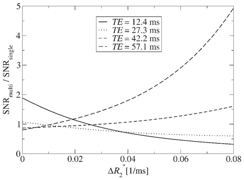
The gain (or loss) of SNR when using PERMEATE in comparison to single-echo parallel imaging with different TEs as a function of tracer concentration

DISCUSSION

The strategy developed to calculate the AIF, i.e. the calculation from the maximum of the first echo and weighted fit together with the automatic selection of arterial voxels, provides a robust estimation of the AIF. That is, it has the appropriate dynamic range for high tracer concentrations (using only the first echo) and the effect of T₁ relaxation is removed in the post-bolus range (using an exponential fit). If only a single echo would be available at TE ≈ 50 ms, CBV and CBF would be overestimated by the confounding additional difference in integral over the AIF time course in Fig. 1(a). Hence, using ME, i.e. having at least an early echo for the AIF estimation and a late echo for typical tracer concentrations in tissue, is crucial for quantitative DSC-MRI. However, a 4-fold overestimation of CBV (and consequently for CBF) values remains, most likely due to a combination of the obstacles mentioned in the Introduction. Each of these sources of error and their impact on CBV/CBF values will be discussed in the following to narrow down the main cause of the overestimation.

The nearly identical integral over AIFs in Fig. 1(d) (maximum abberation 30%) indicates that partial voluming [item (A)] can be ruled out as a source of decisive error at the present spatial resolution, i.e. those obtainable with PI. Otherwise, one would encounter a decrease in AIF amplitude with increasing N because more and more partial voluming would be introduced in case the voxel size exceeds the size of arterial vessels. Thus, the 4-fold overestimation cannot be explained by partial voluming alone.

Most likely, the tissue-dependent and nonlinear relationship between concentration and $\mathrm{\Delta }{R}_2^{\ast }$ [item (B)] is mainly responsible for the overestimation: if an arterial voxel, i.e. one which is selected for AIF calculation, is for the most part composed of blood, the measured $\mathrm{\Delta }{R}_2^{\ast }$ is caused by irreversible relaxation due to molecular interaction and dynamic dephasing/averaging (T₂ relaxation). On the other hand, the dominant contrast mechanism in a typical tissue voxel with a few percent blood is static dephasing due to field inhomogeneities in the extravascular space around the vessels. It has been argued recently on a theoretical basis (5) that the latter relaxation mechanism leads to a 3-fold higher relaxation rate than the former for the same tracer concentration (6). This agrees roughly with our experimental finding of a 4-fold overestimation of CBV and CBF. Thus, use of a uniform linear relationship between concentration and $\mathrm{\Delta }{R}_2^{\ast }$ must be discarded altogether if truly quantitative perfusion analysis based on DSC-MRI should be achieved. Instead, a nonlinear relationship depending on the blood volume fraction must be established. However, it remains unclear why this large discrepancy has not been observed in previous DSC-MRI studies. One explanation would be that the tissue signal in our study is unbiased by T₁ relaxation, which would otherwise diminish the overestimation because it has the opposite effect on CBV and CBF values (see above).

Another reason for the overestimation of CBV and CBF might be that the dynamic range of the first echo is not sufficient for high arterial tracer concentrations [item (C)]. However, the nearly identical AIF amplitude during bolus passage of the first and second echo (with roughly doubled TE) in Fig. 1(a) indicates that this cannot be the main reason for the overestimation. The TE necessary to avoid bias from noise depends on several factors, such as SNR or tracer dose.

Furthermore, because the effect of T₁ relaxation [item (D)] is eliminated using ME, short TRs become possible to increase temporal resolution. Therefore, the course of the residue function is generated with higher fidelity and integration is more accurate than previous attempts with TRs of the order of 1.5–2 s.

Neglecting the dispersion of the bolus during transport from the main arteries to the tissue [item (E)] will distort the MTT (and consequently CBF), but not CBV. As the factor of overestimation is approximately the same for CBV and CBF, this might be a minor effect which cannot explain the overestimation of CBV and CBF.

CONCLUSIONS

The use of multiple echoes is a necessary requirement for truly quantitative DSC-MRI because it extends the dynamic range so that contrast material concentrations, in particular, high arterial concentrations, can be measured with greater accuracy and without bias from T₁ relaxation. In combination with parallel imaging, high temporal and spatial resolutions can be obtained with whole-brain coverage, which in addition to increased quality also helps to circumvent partial voluming when calculating the AIF.

Despite the multiple echo acquisition and the higher scan efficiency, there is no net gain in temporal SNR and, hence, measurement precision between $\mathrm{\Delta }{R}_2^{\ast }$ courses using either single-echo or multi-echo parallel imaging. Overall, if one decides to use parallel imaging, the shortened readouts allow multiple-echo acquisition and much better accuracy at no penalty on precision. One challenge that remains with DSC-MRI and the desire for truly quantitative perfusion imaging is the tissue-dependent nonlinear $\mathrm{\Delta }{R}_2^{\ast }$ dependence upon tracer concentration. Thus, it is necessary to assess the exact dependency by calibration curves obtained from whole blood (4) and simulation using a model of the vascular network (29–35).

Abbreviations used

AIF

arterial input function

CBF

cerebral blood flow

CBV

cerebral blood volume

DSC-MRI

dynamic-susceptibility contrast-based magnetic resonance imaging

FWHM

full-width-at-half-maximum

GM

gray matter

ICA

internal carotid arteries

ME

multi-echo

MTT

mean transit time

PERMEATE

PERfusion with Multiple Echoes And Temporal Enhancement

PI

parallel imaging

SNR

signal-to-noise ratio

WM

white matter

References

- 1.Rempp KA, Brix G, Wenz F, Becker CR, Gückel F, Lorenz WJ. Quantification of regional cerebral blood flow and volume with dynamic susceptibility contrast-enhanced MR imaging. Radiology. 1994;193:637–641. doi: 10.1148/radiology.193.3.7972800. [DOI] [PubMed] [Google Scholar]
- 2.Østergaard L, Weisskoff RM, Chesler DA, Gyldensted C, Rosen BR. High resolution measurement of cerebral blood flow using intravascular tracer bolus passage. Part I: Mathematical approach and statistical analysis. Magn Reson Med. 1996;36:715–725. doi: 10.1002/mrm.1910360510. [DOI] [PubMed] [Google Scholar]
- 3.van Osch MJP, Vonken EPA, Bakker CJG, Viergever MA. Correcting partial volume artifacts of the arterial input function in quantitative cerebral perfusion MRI. Magn Reson Med. 2001;45:477–485. doi: 10.1002/1522-2594(200103)45:3<477::aid-mrm1063>3.0.co;2-4. [DOI] [PubMed] [Google Scholar]
- 4.van Osch MJP, Vonken EPA, Viergever MA, van der Grond J, Bakker CJG. Measuring the arterial input function with gradient echo sequences. Magn Reson Med. 2003;49:1067–1076. doi: 10.1002/mrm.10461. [DOI] [PubMed] [Google Scholar]
- 5.Kiselev VG. On the theoretical basis of perfusion measurements by dynamic susceptibility contrast MRI. Magn Reson Med. 2001;46:1113–1122. doi: 10.1002/mrm.1307. [DOI] [PubMed] [Google Scholar]
- 6.Kiselev VG. Transverse relaxation effect of MRI contrast agents: a crucial issue for quantitative measurement of cerebral perfusion. J Magn Reson Imag. 2005;22:693–696. doi: 10.1002/jmri.20452. [DOI] [PubMed] [Google Scholar]
- 7.Kuperman VY, Karczmar GS, Blomley MJK, Lewis MZ, Lubich LM, Lipton MJ. Differentiating between T1 and T2* changes caused by gadopentetate dimeglumine in the kidney by using a double-echo dynamic MR imaging sequence. J Magn Reson Imag. 1996;6:765–768. doi: 10.1002/jmri.1880060509. [DOI] [PubMed] [Google Scholar]
- 8.Miyati T, Banno T, Mase M, Kasai H, Shundo H, Imazawa M, Ohba S. Dual dynamic contrast-enhanced MR imaging. J Magn Reson Imag. 1997;7:231–235. doi: 10.1002/jmri.1880070136. [DOI] [PubMed] [Google Scholar]
- 9.Vonken EPA, van Osch MJP, Bakker CJG, Viergever MA. Measurement of cerebral perfusion with dual-echo multi-slice quantitative dynamic susceptibility contrast MRI. J Magn Reson Imag. 1999;10:109–117. doi: 10.1002/(sici)1522-2586(199908)10:2<109::aid-jmri1>3.0.co;2-#. [DOI] [PubMed] [Google Scholar]
- 10.Larkman DJ, de Souza NM, Bydder M, Hajnal JV. An investigation into the use of sensitivity-encoded techniques to increase temporal resolution in dynamic contrast-enhanced breast imaging. J Magn Reson Imag. 2001;14:329–335. doi: 10.1002/jmri.1190. [DOI] [PubMed] [Google Scholar]
- 11.Carroll TJ, Rowley HA, Haughton VM. Automatic calculation of the arterial input function for cerebral perfusion imaging with MR imaging. Radiology. 2003;227:593–600. doi: 10.1148/radiol.2272020092. [DOI] [PubMed] [Google Scholar]
- 12.Mlynash M, Eyngorn I, Bammer R, Moseley ME, Tong DC. Automated method for generating the arterial input function on perfusion-weighted MR imaging: validation in patients with stroke. Am J Neuroradiol. 2005;26:1479–1486. [PMC free article] [PubMed] [Google Scholar]
- 13.Newbould RD, Skare ST, Clayton DB, Alley MT, Albers GW, Lansberg M, Bammer R. PERMEATE: High temporal resolution multi-echo/multi-slice dynamic susceptibility contrast perfusion imaging using GRAPPA EPI. ISMRM. 2006;14:673. [Google Scholar]
- 14.Skare S, Bammer R. Spatial modeling of the GRAPPA weights. ISMRM. 2005;13:2422. [Google Scholar]
- 15.Press W, Teukolsky S, Vetterling W, Flannery B. Numerical Recipes in C. 2. Cambridge University Press; Cambridge: 1996. [Google Scholar]
- 16.Wu O, Østergaard L, Weisskoff RM, Brenner T, Rosen BR, Sorensen AG. Tracer arrival timing-insensitive technique for estimating flow in MR perfusion-weighted imaging using singular value decomposition with a block-circulant deconvolution matrix. Magn Reson Med. 2003;50:164–174. doi: 10.1002/mrm.10522. [DOI] [PubMed] [Google Scholar]
- 17.Frackowiak RSJ, Lenzi GL, Jones T, Heather JD. Quantitative measurement of regional cerebral blood flow and oxygen metabolism in man using 15O and positron emission tomography: theory, procedure, and normal values. J Comp Asst Tomogr. 1980;4:727–736. doi: 10.1097/00004728-198012000-00001. [DOI] [PubMed] [Google Scholar]
- 18.Lenzi GL, Frackowiak RSJ, Jones T, Heather JD, Lammertsma AA, Rhodes C, Pozzilli C. CMRO2 and CBF by the oxygen-15 inhalation technique. Eur Neurol. 1981;20:285–290. doi: 10.1159/000115248. [DOI] [PubMed] [Google Scholar]
- 19.Meyer JS, Hayman LA, Amano T, Nakajima S, Shaw T, Lauzon P, Derman S, Karacan I, Harati Y. Mapping local blood flow of human brain by CT scanning during stable xenon inhalation. Stroke. 1981;12:426–336. doi: 10.1161/01.str.12.4.426. [DOI] [PubMed] [Google Scholar]
- 20.Pantano P, Baron JC, Lebrun-Grandié P, Duquesnoy N, Bousser MG, Comar D. Regional cerebral blood flow and oxygen consumption in human aging. Stroke. 1984;15:635–641. doi: 10.1161/01.str.15.4.635. [DOI] [PubMed] [Google Scholar]
- 21.Brooks DJ, Beaney RP, Leenders KL, Marshall J, Thomas DJ, Jones T. Regional cerebral oxygen utilization, blood flow and blood volume in benign intracranial hypertension studied by positron emission tomography. Neurology. 1985;35:1030–1034. doi: 10.1212/wnl.35.7.1030. [DOI] [PubMed] [Google Scholar]
- 22.Leendres KL, Perani D, Lammertsma AA, Heather JD, Buckingham P, Healy MJR, Gibbs JM, Wise RJS, Hatazawa J, Herold S, Beaney RP, Brooks DJ, Spinks T, Rhodes C, Frackowiak RSJ, Jones T. Cerebral blood flow, blood volume and oxygen utilization, normal values and effect of age. Brain. 1990;113:27–47. doi: 10.1093/brain/113.1.27. [DOI] [PubMed] [Google Scholar]
- 23.Kuppusamy K, Lin W, Cizek GR, Haacke EM. In vivo regional cerebral blood volume: Quantitative assessment with 3D T1-weighted pre- and postcontrast MR imaging. Radiology. 1996;201:106–112. doi: 10.1148/radiology.201.1.8816529. [DOI] [PubMed] [Google Scholar]
- 24.Law I, Iida H, Holm S, Nour S, Rostrup E, Svarer C, Paulson OB. Quantitation of regional cerebral blood flow corrected for partial volume effect using O-15 water and PET: II. normal values and gray matter blood flow response to visual activation. J Cereb Blood Flow Metab. 2000;20:1252–1263. doi: 10.1097/00004647-200008000-00010. [DOI] [PubMed] [Google Scholar]
- 25.Kudo K, Terae S, Katoh C, Oka M, Shiga T, Tamaki N, Miyasaka K. Quantitative cerebral blood flow measurement with dynamic perfusion CT using the vascular-pixel elimination method: Comparison with positron emission tomography. Am J Neuroradiol. 2003;24:419–426. [PMC free article] [PubMed] [Google Scholar]
- 26.Muizelaar JP, Fatouros PP, Schröder ML. A new method for quantitative regional cerebral blood volume measurements using computer tomography. Stroke. 2003;28:1998–2005. doi: 10.1161/01.str.28.10.1998. [DOI] [PubMed] [Google Scholar]
- 27.Lu H, Law M, Johnson G, Ge Y, van Zijl PCM, Helpern JA. Novel approach to the measurement of absolute cerebral blood volume using vascular-space-occupancy magnetic resonance imaging. Magn Reson Med. 2005;54:1403–1411. doi: 10.1002/mrm.20705. [DOI] [PubMed] [Google Scholar]
- 28.Rostrup E, Knudsen GM, Law I, Holm S, Larsson HBW, Paulson OB. The relationship between cerebral blood flow and volume in humans. NeuroImage. 2005;24:1–11. doi: 10.1016/j.neuroimage.2004.09.043. [DOI] [PubMed] [Google Scholar]
- 29.Fisel CR, Ackerman JL, Buxton RB, Garrido L, Belliveau JW, Rosen BR, Brady TJ. MR contrast due to microscopically heterogenous magnetic susceptibility: numerical simulations and applications to cerebral physiology. Magn Reson Med. 1991;17:336–347. doi: 10.1002/mrm.1910170206. [DOI] [PubMed] [Google Scholar]
- 30.Weisskoff RM, Zuo CS, Boxerman JL, Rosen BP. Microscopic susceptibility variation and transverse relaxation: Theory and experiment. Magn Reson Med. 1994;31:601–610. doi: 10.1002/mrm.1910310605. [DOI] [PubMed] [Google Scholar]
- 31.Kennan RP, Zhong J, Gore JC. Intravascular susceptibility contrast mechanisms in tissues. Magn Reson Med. 1994;31:9–21. doi: 10.1002/mrm.1910310103. [DOI] [PubMed] [Google Scholar]
- 32.Boxerman JL, Hamberg LM, Rosen BP, Weisskoff RM. MR contrast due to intravascular magnetic susceptibility perturbations. Magn Reson Med. 1995;34:555–566. doi: 10.1002/mrm.1910340412. [DOI] [PubMed] [Google Scholar]
- 33.Bandettini PA, Wong EC. Effects of biophysical and physiologic parameters on brain activation-induced R2* and R2 changes: simulations using a deterministic diffusion model. Intl J Imag Sys Techn. 1995;6:133–152. [Google Scholar]
- 34.Kiselev VG, Posse S. Analytical model of susceptibility-induced MR signal dephasing: effect of diffusion in a microvascular network. Magn Reson Med. 1999;41:499–509. doi: 10.1002/(sici)1522-2594(199903)41:3<499::aid-mrm12>3.0.co;2-o. [DOI] [PubMed] [Google Scholar]
- 35.Fujita N. Extravascular contributions of blood oxygenation level-dependent signal changes: A numerical analysis based on a vascular network model. Magn Reson Med. 2001;46:723–734. doi: 10.1002/mrm.1251. [DOI] [PubMed] [Google Scholar]