Modeling and incorporating cardiac-induced lung tissue motion in a breathing motion model

Abstract

Purpose: The purpose of this work is to develop a cardiac-induced lung motion model to be integrated into an existing breathing motion model.

Methods: The authors’ proposed cardiac-induced lung motion model represents the lung tissue's specific response to the subject's cardiac cycle. The model is mathematically defined as a product of a converging polynomial function h of the cardiac phase (c) and the maximum displacement $\stackrel{\rightharpoonup }{\gamma }\left({\stackrel{\rightharpoonup }{X}}_0\right)$ of each voxel (${\stackrel{\rightharpoonup }{X}}_0$) among all the cardiac phases. The function h(c) was estimated from cardiac-gated MR imaging of ten healthy volunteers using an Akaike Information Criteria optimization algorithm. For each volunteer, a total of 24 short-axis and 18 radial planar views were acquired on a 1.5 T MR scanner during a series of 12–15 s breath-hold maneuvers. Each view contained 30 temporal frames of equal time-duration beginning with the end-diastolic cardiac phase. The frames in each of the planar views were resampled to create a set of three-dimensional (3D) anatomical volumes representing thoracic anatomy at different cardiac phases. A 3D multiresolution optical flow deformable image registration algorithm was used to quantify the difference in tissue position between the end-diastolic cardiac phase and the remaining cardiac phases. To account for image noise, voxel displacements whose maximum values were less than 0.3 mm, were excluded. In addition, the blood vessels were segmented and excluded in order to eliminate registration artifacts caused by blood-flow.

Results: The average cardiac-induced lung motions for displacements greater than 0.3 mm were found to be 0.86 ± 0.74 and 0.97 ± 0.93 mm in the left and right lungs, respectively. The average model residual error for the ten healthy volunteers was found to be 0.29 ± 0.08 mm in the left lung and 0.38 ± 0.14 mm in the right lung for tissue displacements greater than 0.3 mm. The relative error decreased with increasing cardiac-induced lung tissue motion. While the relative error was > 60% for submillimeter cardiac-induced lung tissue motion, the relative error decreased to < 5% for cardiac-induced lung tissue motion that exceeded 10 mm in displacement.

Conclusions: The authors’ studies implied that modeling and including cardiac-induced lung motion would improve breathing motion model accuracy for tissues with cardiac-induced motion greater than 0.3 mm.

INTRODUCTION

Breathing motion adversely impacts the radiation therapy treatment planning and delivery process.¹ It can arise from voluntary, involuntary, and semivoluntary physiological factors. One solution to account for the breathing-induced lung tissue motion has been to employ lung motion models for planning and treatment.^{2, 3, 4, 5, 6, 7, 8, 9, 10, 11, 12, 13} Lung and lung tumor motion models have been developed based on lung tissue elasticity,^{2, 8, 11, 12, 13} respiratory phase,^{3, 5, 6, 7, 9} and biomechanical tissue properties.^{4, 10} These models, however, did not address the lung motion induced by the heart's pulsatile motion. There have been studies that evaluated breathing induced cardiac motion,^{14, 15, 16, 17} but no specific modeling efforts have been developed to quantify and report cardiac-induced lung motion.

Cardiac motion is uncorrelated to the breathing cycle, so cardiac motion may appear as noise in breathing motion measurements that consist of repeated CT scans, such as those used by Low et al.¹⁸ Subsequently, breathing motion model accuracy will be degraded by this apparently random motion component. Cardiac-induced lung tissue motion has been measured using 4D fluoroscopy and observed to be oriented in the lateral direction with a magnitude in the range of 1–4 mm.⁶

The motion of the heart during the different cardiac phases consists of radial, longitudinal, and circumferential displacements.^{19, 20, 21, 22} The base of the heart contracts, ejecting blood from the ventricles. This contraction changes the shape and volume of the heart, causing the lung to expand and slide against the heart. The apex of the heart contracts less than the base but includes a circumferential torsion.²³ The maximum myocardium displacement of the heart during the different phases of a cardiac cycle has been reported to be approximately 30 mm, greater than the 1–4 mm of lung-induced cardiac motion.²⁴ Such large displacements may also lead to substantial cardiac-induced lung motion. Modeling the cardiac-induced lung motion and incorporating the cardiac-induced lung motion into a breathing lung motion model^{4, 10, 25, 26} forms the focus of this paper.

METHODS

In this section, we describe the mathematical formulation to model cardiac-induced lung tissue motion. The formulation, when incorporated into the 5D breathing motion model accounts for cardiac-induced lung motion and presumably will improve the breathing motion model. To characterize the morphological changes in lung anatomy during the cardiac cycle, we employed a cardiac-gated MRI protocol. A three-dimensional (3D) optical flow image registration algorithm was used to find the deformation vectors of the lung tissue in Cartesian space. The temporal dependence of the deformation vectors on the cardiac cycle was estimated with a converging polynomial whose order was optimized with an Akaike Information Criteria (AIC) method.²⁷ The model was designed as a linear relation between the maximum tissue displacement of each voxel and the cardiac phase. The model performance was assessed by comparing the model residual error against the uncompensated cardiac-induced lung tissue motion.

5D breathing motion model

The breathing motion model that we were modifying was previously developed by Low et al.⁴ The model utilized airflow f and tidal volume v as time-dependent surrogates and the internal lung tissue position ($\stackrel{\rightharpoonup }{X}$) was determined by the expression⁴

$$\stackrel{\rightharpoonup }{X}\left(v,f:{\stackrel{\rightharpoonup }{X}}_0\right)={\stackrel{\rightharpoonup }{X}}_0+\stackrel{\rightharpoonup }{\alpha }\left({\stackrel{\rightharpoonup }{X}}_0\right)v+\stackrel{\rightharpoonup }{\beta }\left({\stackrel{\rightharpoonup }{X}}_0\right)f,$$ (1)

where ${\stackrel{\rightharpoonup }{X}}_0$ was the position of the tissue at zero tidal volume and airflow. v and f scaled the tissue specific vectors $\stackrel{\rightharpoonup }{\alpha }$ and $\stackrel{\rightharpoonup }{\beta }$ which determined the motion direction and magnitude for the volume filling and hysteresis components, respectively.

The accuracy of determining $\stackrel{\rightharpoonup }{\alpha }$ and $\stackrel{\rightharpoonup }{\beta }$ in the 5D breathing motion model was previously demonstrated in a cohort of 50 subjects.²⁵ Model and measured tissue position differences were used by Zhao et al.²⁶ to evaluate the 5D model precision. They showed that the absolute discrepancy of the 5D breathing motion model was less than 2.1 mm for 90% of the voxels in the subject cohort,²⁶ but their measurements may not have had sufficient resolution to detect increased modeling errors near the heart. More recently, Low et al.¹⁸ improved the breathing motion model measurement technique and saw increased motion model error near the heart that might be decreased if a cardiac motion model term was incorporated into the breathing motion model.

Cardiac-induced lung motion model

To model the effect of the cardiac motion on lung tissue, we introduced a new term to Eq. 1. For clarity, definitions of the variables and terms used in this section are presented in Table 1. We modeled the cardiac-induced lung motion as follows:

$$\stackrel{\rightharpoonup }{C}=\stackrel{\rightharpoonup }{\gamma }\left({\stackrel{\rightharpoonup }{X}}_0\right)h\left(c\right),$$ (2)

where $\stackrel{\rightharpoonup }{C}$ represented the cardiac-induced lung motion at any cardiac phase, and ${\stackrel{\rightharpoonup }{X}}_0$ was the position of the tissue at v = f = 0 and at the beginning of the cardiac cycle (c = 0). h(c) described the temporal motion magnitude bin of all of the cardiac-induced motion and $\stackrel{\rightharpoonup }{\gamma }\left({\stackrel{\rightharpoonup }{X}}_0\right)$ described the local motion magnitude and direction. h(c) was defined such that h(0) = 0 and the maximum value for h was 1.

Table 1.

Table of variables introduced in this paper.

Variable	Meaning
$\stackrel{\rightharpoonup }{X}$	Lung tissue position
${\stackrel{\rightharpoonup }{X}}_0$	Initial lung tissue position
$\stackrel{\rightharpoonup }{\alpha }$	Lung tissue specific response to volume filling
v	Tidal volume
$\stackrel{\rightharpoonup }{\beta }$	Lung tissue specific response to hysteresis
f	Airflow
$\stackrel{\rightharpoonup }{C}$	Cardiac-induced lung motion term
$\stackrel{\rightharpoonup }{\gamma }$	Lung tissue specific response to the cardiac motion
H	Lung tissue response to the cardiac cycle
C	Cardiac phase
$\left(\stackrel{\rightharpoonup }{u},\stackrel{\rightharpoonup }{v},\stackrel{\rightharpoonup }{w}\right)$	Deformation vectors
$\left(\widehat{i},\widehat{j},\widehat{k}\right)$	Cartesian coordinate system of $\stackrel{\rightharpoonup }{\gamma }$
(θx, θy, θz)	Cartesian coordinate system angles of $\stackrel{\rightharpoonup }{\gamma }$
AIC	Akaike Information Criteria
k	Number of parameters in h
T	Total number of cardiac frames in a single cardiac cycle
L	Maximum likelihood
${\sigma }_c^2$	Variance at a given cardiac frame
$h_c^{\mathrm{fit}}$	h value from the polynomial fit at a given cardiac frame
$h_c^m$	h value at the a given cardiac frame
χ2	Chi-squared
A	constant under the condition of consistent measurement data
s	Subject
n	Number of voxels
j	Number of coefficients
m	Polynomial coefficient

From a biomechanical perspective, the term $\stackrel{\rightharpoonup }{\gamma }$ represented the tissue specific response to the cardiac pulsation. The term was assumed to be independent of breathing-induced motion and so the term was added to the 5D model shown in Eq. 1. In Cartesian coordinates, $\stackrel{\rightharpoonup }{\gamma }$ was written as

$$\stackrel{\rightharpoonup }{\gamma }=\Vert \stackrel{\rightharpoonup }{\gamma }\Vert \left(\cos {\theta }_x\widehat{i}+\cos {\theta }_y\widehat{j}+\cos {\theta }_z\widehat{k}\right),$$ (3)

where $\Vert \stackrel{\rightharpoonup }{\gamma }\Vert$ was the maximum displacement of the lung tissue during the cardiac cycle and was formulated as follows:

$$\Vert \stackrel{\rightharpoonup }{\gamma }\Vert =\max \{\Vert {\stackrel{\rightharpoonup }{u}}_p\widehat{i}+{\stackrel{\rightharpoonup }{v}}_p\widehat{j}+{\stackrel{\rightharpoonup }{w}}_p\widehat{k}{\Vert \}}_{c=1}^T,$$ (4)

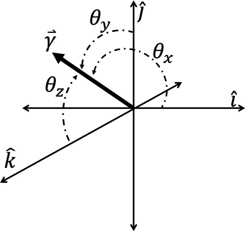
where the term $\left(\stackrel{\rightharpoonup }{u},\stackrel{\rightharpoonup }{v},\stackrel{\rightharpoonup }{w}\right)$ indicated the deformation vectors for each voxel across the cardiac frames in the Cartesian coordinate system $\left(\widehat{i},\widehat{j},\widehat{k}\right)$. The superscript T denotes the total number of cardiac frames (c) in a single cardiac cycle. The values of (θ_x, θ_y, θ_z) were determined from

$$\begin{array}{ccc}\hfill {\theta }_x& =& {\cos }^{-1}\left(\frac{\Vert \stackrel{\rightharpoonup }{u}{\Vert }_{\max }}{\Vert \stackrel{\rightharpoonup }{\gamma }\Vert }\right),{\theta }_y={\cos }^{-1}\left(\frac{\Vert \stackrel{\rightharpoonup }{v}{\Vert }_{\max }}{\Vert \stackrel{\rightharpoonup }{\gamma }\Vert }\right),\hfill \\ \hfill {\theta }_z& =& {\cos }^{-1}\left(\frac{\Vert \stackrel{\rightharpoonup }{w}{\Vert }_{\max }}{\Vert \stackrel{\rightharpoonup }{\gamma }\Vert }\right).\hfill \end{array}$$ (5)

Figure 1 illustrates the coordinate system of the cardiac-induced lung motion model.

Figure 1.

Coordinate system for the cardiac-induced lung motion model.

The temporal term h(c) was represented in the form of a converging polynomial that fitted the deformation vector magnitudes normalized to the maximum tissue displacement. The polynomial order was chosen as the lowest order polynomial function capable of describing the normalized deformation vector magnitudes while satisfying the AIC.²⁷ For this study, the AIC was expressed in terms of the number of parameters (k) in the polynomial fit of h and the maximum likelihood (L). The expression for the AIC and the maximum likelihood are shown in Eqs. 6, 7, respectively,²⁷

$$\mathrm{AIC}=2k-2\ln \left(L\right),$$ (6)

$$\begin{array}{c}\hfill L={\prod }_{c=1}^T{\left(\frac{1}{2\pi {\sigma }_c^2}\right)}^{1/2}\exp \left(-{\sum }_{c=1}^T\frac{{\left(h_c^{\mathrm{fit}}-h_c^m\right)}^2}{2{\sigma }_c^2}\right),\end{array}$$ (7)

where ${\sigma }_c^2$ is the variance at a given cardiac frame, $h_c^{\mathrm{fit}}$ is the h value from the polynomial fit at a given cardiac frame, and $h_c^m$ is the measured h value at a given cardiac frame. An expression for the AIC in terms of chi-squared (χ²) was derived by taking the natural log of the maximum likelihood expressed in Eq. 7²⁷

$$\begin{array}{ccc}\hfill \ln \left(L\right)& =& \ln \left[{\prod }_{c=1}^T{\left(\frac{1}{2\pi {\sigma }_c^2}\right)}^{1/2}\right]-\frac{1}{2}{\sum }_{c=1}^T\frac{{\left(h_c^{\mathrm{fit}}-h_c^m\right)}^2}{2{\sigma }_c^2}\hfill \\ & =& A-\frac{1}{2}{\chi }^2,\hfill \end{array}$$ (8)

where the first term in Eq. 8, A, is a constant under the condition of consistent measurement data (i.e., the number of model parameter varies but the measured data stay the same) and the second term is the chi-squared expression. The AIC was used to find the fewest number of parameters needed to describe the behavior of h over the cardiac cycle through an exhaustive search, since A was independent of the fit it was omitted from the AIC expression. This allowed the AIC to be a straightforward function of the number of parameters in the polynomial fit of h and the chi-squared expression.²⁸

A polynomial function was chosen to maintain a strictly temporal relationship between cardiac frame and lung tissue motion. The deformation vectors of each voxel were normalized to the maximum displacement of that voxel over the cardiac cycle. The first cardiac frame of h was defined to be 0 since this cardiac frame was taken as the reference image in the deformable image registration algorithm. The value of h was made to vary between 0, corresponding to the reference cardiac phase (end-diastolic), and 1 which corresponded to the cardiac frame with greatest tissue motion. The volunteer specific (s) polynomial behavior of h for each voxel (n) followed the form

$$h_n^s\left(c\right)={\sum }_{j=0}^k{m}_j{c}^j.$$ (9)

A mean of the polynomial coefficients for each voxel was calculated to produce a single new polynomial for all of the voxels within the lung

$$h^s\left(c\right)=\frac{1}{n}{\sum }_{j=1}^n{h}_k^s\left(c\right).$$ (10)

This procedure to determine h was individually done for the right and left lungs. The limit of $\stackrel{\rightharpoonup }{C}$ provided in this section was mathematically undefined in the event that a given voxel did not move, $\Vert \stackrel{\rightharpoonup }{C}\Vert =0$. A lung voxel was considered to be stationary during the cardiac cycle based on the magnitude of the deformation vectors calculated by the deformable image registration algorithm. If a voxel did not experience cardiac-induced lung motion, $\Vert \stackrel{\rightharpoonup }{\gamma }\Vert$ and h would be equal to 0 and the angular components of $\Vert \stackrel{\rightharpoonup }{\gamma }\Vert$, (θ_x, θ_y, θ_z) would be undefined. Incorporating the cardiac-induced lung motion term ($\stackrel{\rightharpoonup }{C}$) from Eq. 2 into Eq. 1 provided

$$\stackrel{\rightharpoonup }{X}\left(v,f,h:{\stackrel{\rightharpoonup }{X}}_0\right)=\left\{\begin{array}{cc}\hfill {\stackrel{\rightharpoonup }{X}}_0+\stackrel{\rightharpoonup }{\alpha }\left({\stackrel{\rightharpoonup }{X}}_0\right)v+\stackrel{\rightharpoonup }{\beta }\left({\stackrel{\rightharpoonup }{X}}_0\right)f& \hfill \exists \stackrel{\rightharpoonup }{C}|\Vert \stackrel{\rightharpoonup }{\gamma }\Vert =0\\ \hfill {\stackrel{\rightharpoonup }{X}}_0+\stackrel{\rightharpoonup }{\alpha }\left({\stackrel{\rightharpoonup }{X}}_0\right)v+\stackrel{\rightharpoonup }{\beta }\left({\stackrel{\rightharpoonup }{X}}_0\right)f+\stackrel{\rightharpoonup }{C}& \hfill \exists \stackrel{\rightharpoonup }{C}|\Vert \stackrel{\rightharpoonup }{\gamma }\Vert >0\end{array}\right..$$ (11)

Data collection

To quantify cardiac-induced lung motion, we used a MRI protocol to measure lung tissue motion during the cardiac cycle. Ten healthy volunteers were imaged with an Avanto 1.5 T Siemens MRI scanner (Siemens Healthcare, Erlangen, Germany). The imaging protocol closely followed a previously established sequence by Ennis et al.²⁹ The protocol was a balanced steady-state free precession sequence with an echo time of 1.6 ms and a repetition time of 3.2 ms. The field of view was 360 mm. The volunteers were instructed to perform a series of 12–15 s breath holds at midexhalation for each view. The views were acquired with electrocardiogram (ECG) gating to monitor the cardiac phase. For each view, ∼14 cardiac cycles of data were acquired with each breath hold and were retrospectively binned using the ECG tags to provide 30 equal time duration cardiac frames to represent a single cardiac cycle. The first cardiac frame represented the thoracic anatomy at the end diastolic cardiac phase and was timed to coincide with the closure of the mitral valve. A total of 24 planar views in the short axis orientation were taken with 3.5–4 mm slice thickness from the mitral valve plane at the base of the heart to the ventricular apex plane at the apex of the heart. The slice thickness was directly related to the short axis length of the volunteer's heart. The short axis views were supplemented by 18 radial views at 20° increments centered about the plane intersecting the mitral valve and the ventricular apex. The short axis images and the radial images were resampled to form a 3D volume representing the thorax anatomy at each cardiac frame and provided the input for a 3D deformable image registration algorithm. The right and left lung volumes were masked with a region growing algorithm to only consider lung tissue in the analysis. Large blood vessels and rigid bronchial structures were also removed to avoid MRI perfusion artifacts.

Image registration

We employed a Graphics Processing Unit (GPU) based multiresolution 3D optical flow algorithm.^{30, 31} Mathematically, the optical flow image registration method was based on the Taylor Series approximation and has been well defined in literature.^{30, 31} Solving for this Taylor series approximation, we employed a Jacobian iterative solver^{30, 31} that was computationally accelerated to determine the 3D volumetric displacement.

The registration steps were: For each subject, the 3D anatomy at the end-diastole cardiac phase was taken as a reference and the deformation vectors were determined from the reference 3D anatomy to the 3D anatomies at different cardiac phases. A set of 3D anatomies at multiple lower resolutions were generated for both the reference and the target 3D anatomy. The registration was performed for the reference and the target 3D anatomy at the lowest 3D resolution level. The result of this registration was upscaled and provided as initial input for registering the reference and the target 3D anatomy at the next 3D resolution level. The process continued until the reference and the target 3D anatomy were registered at the original 3D resolution level.

Model generation

The results of the multiresolution 3D optical flow registration provided the deformation vectors for each voxel in the lung. The segmented lung volumes without internal blood vessels provided the regions of interest in the thoracic anatomy. The maximum displacement over the cardiac cycle relative to the first frame for each voxel was identified. This was used to normalize the response of the voxel to the cardiac cycle over the 30 cardiac phases. A converging polynomial was fit to the normalized response for each voxel from the reference phase (h = 0) to the maximum displacement phase (h = 1). The polynomial coefficients of each voxel were individually averaged over all voxels in the lung to express a single polynomial for the lung. The polynomial was used to scale the maximum displacement along the direction of the maximum displacement of each voxel over the cardiac cycle to create the cardiac-induced lung motion model.

Statistical distribution

The displacement magnitude and direction for each lung voxel were analyzed to check the data distribution and assess statistical significance. An Ansari–Bradley test was selected as a statistical metric with which to assess the distribution of $\Vert \stackrel{\rightharpoonup }{\gamma }\Vert$ and the model residual error. The Ansari–Bradley test is a nonparametric hypothesis test of equal variances. The distribution of $\Vert \stackrel{\rightharpoonup }{\gamma }\Vert$ was checked at the 95% confidence level.

RESULTS

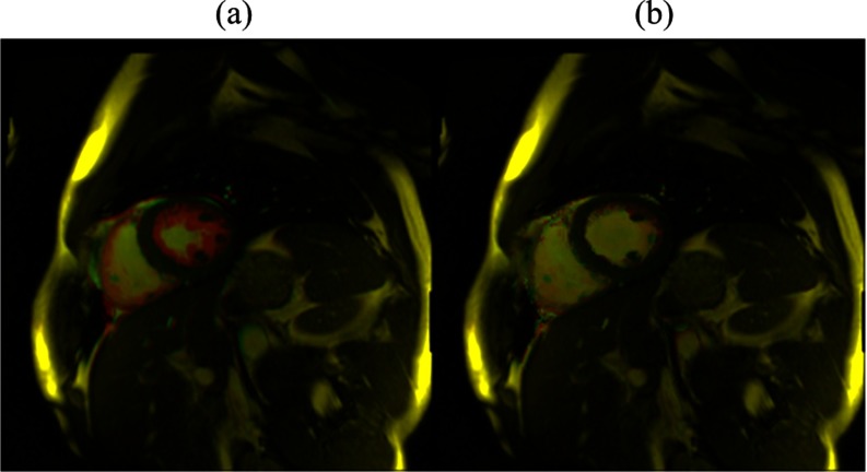
The deformable image registration algorithm accuracy was evaluated using the calculated deformation vectors to warp each cardiac frame back to its respective reference. The discrepancy between the reference cardiac frame and subsequent cardiac frames with this method was observed to be negligible. Figure 2 shows the overlay of the reference and one of the cardiac frame images for both warped and unwarped cases. This example shows the deformable image registration algorithm to be qualitatively accurate. A quantitative analysis for the accuracy of the deformable image registration algorithm has been described in detail in Santhanam et al.³² That paper found the deformable image registration algorithm average error to be 0.36 ± 0.06 mm based on 20 landmarks within the lungs. The average error was greatly influenced by the slice thickness of the MR images since the measured cardiac-induced lung displacement was small relative to the slice thickness.

Figure 2.

Figure 2(a) shows an overlay example of the reference cardiac frame image with a randomly selected cardiac frame. In Fig. 2(b), the randomly selected cardiac frame warped by the calculated deformation vectors overlaid with the reference cardiac frame is shown. The highlighted pixels display the discrepancy between the reference and randomly selected cardiac frames.

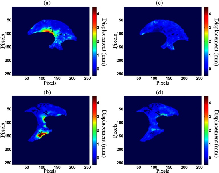
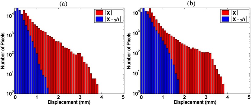
The average cardiac-induced lung motion for tissue displacements greater than 0.3 mm was 0.86 ± 0.74 and 0.97 ± 0.93 mm in the left and right lungs, respectively. The average model residual error, defined as the difference between the measured cardiac induced motion and $\vec{C}$, for the ten healthy volunteers was found to be 0.29 ± 0.08 mm in the left lung and 0.38 ± 0.14 mm in the right lung for tissue displacements greater than 0.3 mm. Figure 3 shows the reduction in cardiac-induced lung motion achieved with the model for a short axis view of the right and left lungs. Figures 3a, 3b illustrate the distribution of the cardiac-induced lung tissue motion in the right and left lungs, respectively, showing that the cardiac-induced motion was submillimeter for most of the lung tissue. Figures 3c, 3d show the corresponding distribution of the model residual error, defined as the difference between the registration-measured motion and the motion described by $\vec{C}$, for the views in Figs. 3a, 3b, respectively. Every voxel had less model residual error compared with the magnitude of cardiac-induced lung tissue motion. This is illustrated in Fig. 4 by comparing the distribution of the cardiac-induced lung motion and the model residual error. Figures 4a, 4b show histograms of the motion magnitudes for the left and right lungs, respectively. In each figure, the uncompensated motion is tabulated as are the model residual errors. Ideally, the model residual errors would all be zero, but they were not due, in part, to the simplification of the model that the motion temporal magnitude bin was constant throughout the lungs, and, in part, to image registration errors. As shown by the model residual error, the cardiac motion was modeled to within 1 mm of its actual motion in this slice. The actual maximum motion was four times greater than the maximum residual error. An overall comparison between the cardiac-induced lung tissue motion and the model residual error for the ten healthy subjects is shown in Fig. 5, highlighting the model quality. To quantify the accuracy of the model in describing cardiac-induced lung tissue motion, the average relative errors for increasing motion magnitude bins were calculated. The results of this method are shown in Tables 2, 3. Table 2 reports the summary of the model's average absolute and average relative error for the right and left lungs over various tissue trajectory motion magnitude bins. Table 3 reports the average cardiac-induced motion and the model residual error for the right and left lungs.

Figure 3.

The uncompensated cardiac-induced lung tissue motion is shown for a SA view of the left lung (a) and right lung (b). The corresponding model residual error is shown for the left lung (c) and the right lung (d).

Figure 4.

A sample distribution comparison between the uncompensated cardiac-induced lung tissue motion $|\stackrel{\rightharpoonup }{X}|$ and the model residual error $|\stackrel{\rightharpoonup }{X}-\stackrel{\rightharpoonup }{\gamma }h|$ for the left lung (a) and the right lung (b) shown in Fig. 3.

Figure 5.

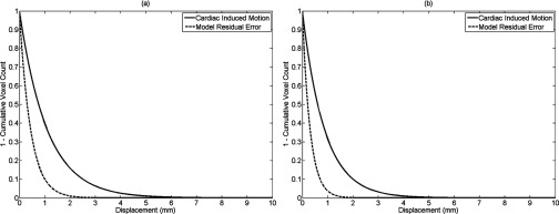
Cumulative histogram comparison between the cardiac-induced lung tissue motion and the model residual error for all voxels in the right (a) and left (b) lungs.

Table 2.

Summary of the average absolute error and average relative error for increasing cardiac-induced lung motion magnitude bins.

Motion magnitude bin (mm)	Left lung average absolute error (mm)	Left lung relative error	Right lung average absolute error (mm)	Right lung relative error
0.3–1	0.30 ± 0. 09	59.8 ± 35.8%	0.45 ± 0.20	75.4 ± 56.9%
1–2	0.33 ± 0.11	24.9 ± 6.2%	0.53 ± 0.28	34.3 ± 11.8%
2–3	0.32 ± 0.10	13.7 ± 1.2%	0.58 ± 0.34	20.0 ± 4.0%
3–4	0.32 ± 0.11	9.6 ± 0.9%	0.61 ± 0.38	14.2 ± 2.0%
4–5	0.34 ± 0.12	7.7 ± 0.6%	0.61 ± 0.37	11.0 ± 1.2%
5–6	0.35 ± 0.12	6.4 ± 0.4%	0.58 ± 0.33	8.8 ± 0.8%
6–7	0.34 ± 0.12	5.3 ± 0.3%	0.57 ± 0.33	7.0 ± 0.5%
7–8	0.35 ± 0.12	4.7 ± 0.2%	0.56 ± 0.32	5.6 ± 0.3%
8–9	0.35 ± 0.12	4.2 ± 0.2%	0.55 ± 0.30	4.9 ± 0.2%
9–10	0.36 ± 0.13	3.8 ± 0.2%	0.56 ± 0.31	4.2 ± 0.2%
> 10	0.38 ± 0.14	3.4 ± 0.1%	0.60 ± 0.36	3.5 ± 0.1%

Table 3.

Summary of average cardiac-induced lung tissue motion and average model residual error for the right and left lungs over all subjects in this study.

Subject	Average cardiac induced motion, left lung (mm)	Average residual error left lung (mm)	Average cardiac induced motion, right lung (mm)	Average residual error right lung (mm)
1	0.69 ± 0.47	0.21 ± 0.04	0.80 ± 0.64	0.26 ± 0.07
2	0.75 ± 0.56	0.23 ± 0.05	0.69 ± 0.48	0.31 ± 0.09
3	0.67 ± 0.45	0.23 ± 0.05	0.68 ± 0.46	0.28 ± 0.08
4	0.66 ± 0.43	0.20 ± 0.04	0.65 ± 0.42	0.23 ± 0.05
5	0.83 ± 0.69	0.43 ± 0.18	0.72 ± 0.52	0.27 ± 0.07
6	1.00 ± 0.99	0.31 ± 0.10	1.17 ± 1.36	0.48 ± 0.23
7	1.01 ± 1.02	0.33 ± 0.11	1.18 ± 1.40	0.54 ± 0.29
8	0.63 ± 0.40	0.23 ± 0.05	0.60 ± 0.36	0.25 ± 0.06
9	1.05 ± 0.53	0.31 ± 0.18	1.14 ± 1.30	0.51 ± 0.26
10	1.07 ± 1.14	0.39 ± 0.15	1.58 ± 2.51	0.67 ± 0.44

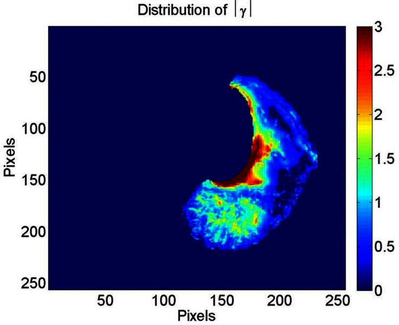
$\Vert \stackrel{\rightharpoonup }{\gamma }\Vert$ was found to vary smoothly throughout the lung. Figure 6 shows a typical example of the $\Vert \stackrel{\rightharpoonup }{\gamma }\Vert$ for a SA view of the left lung. The cardiac-induced lung tissue motion was observed to be greater than 1 mm for 15.5% of the voxels analyzed in this study. These voxels were almost exclusively located in lung regions close to the heart. A rapid decrease in the cardiac-induced lung tissue motion magnitude was observed outside of this region. Based on an Ansari–Bradley test, the results for the cardiac-induced lung tissue motion (p < 0.01), $\Vert \stackrel{\rightharpoonup }{\gamma }\Vert$ (p < 0.04), and the model residual error (p < 0.01) were found to follow an exponential distribution.

Figure 6.

A typical example of $\stackrel{\rightharpoonup }{\gamma }$ for a SA view of the left lung. The intensity scale is in units of mm.

Based on the AIC analysis, a ninth order polynomial was found to be the lowest order required to describe the magnitude of lung tissue displacement in each cardiac frame for each voxel. The behavior of h over the lung for each subject was similar in the right and left lungs individually for the ten healthy volunteers. Figure 7 shows the behavior of h over the cardiac cycle for the right and left lungs for the ten healthy subjects.

Figure 7.

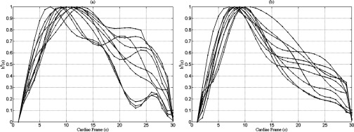
h curves for the right (a) and left (b) lungs for the ten subjects.

The accuracy and the robustness of the analysis are greatly dependent on the accuracy of the DIR algorithm. We validated the DIR algorithm using a landmark-based Target Registration Error (TRE) metric. A set of 80 landmarks was tracked on each of the ten datasets from the end-systolic to end-diastolic phase. Figure 8 presents the user interface that we employed for our validation process. The landmarks were placed by an expert on the reference cardiac phase data (left) as shown by the cross hairs. For each of the landmarks, the corresponding landmark in the target phase was calculated using the DIR results and were visually shown to the expert as cross hairs overlapping the target (right) image. Based on the results, the expert either accepted the DIR results or marked the correct landmark on the target image. Once the 80 landmarks were found, the TRE for each of the datasets was computed. Table 4 tabulates the DIR registration results. For each of the datasets, the TRE was found to be subvoxel and in the range of 0.27–1.1 mm. The registration accuracy enabled the cardiac-induced lung tissue motion model to not be influenced by errors in DIR.

Figure 8.

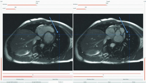
User interface for the DIR validation process. The corresponding landmark locations are denoted by arrows on the reference cardiac phase data (left) and on the target phase image (right).

Table 4.

Mean error of the DIR for each subject from the landmark validation process.

	Subject	Mean target registration error (mm)
	1	0.612
	2	0.92
	3	0.279
	4	0.463
	5	1.16
	6	0.824
	7	0.96
	8	1.03
	9	1.10
	10	0.83

DISCUSSION

This paper has proposed a new term for the 5D breathing motion model⁴ to account for cardiac-induced lung tissue motion. The cardiac-induced lung tissue motion term followed the form of the other terms in the 5D breathing motion model. The key concept behind the 5D breathing motion model was that it separated the motion of lung tissue into unique motion sources. The original 5D breathing motion model had two components, a lung filling component and a breathing rate component. Each component was approximated to be independent in the model. The breathing rate component was intended to model hysteresis motion, which was hypothesized to be due to pressure imbalances within the lungs, and these were hypothesized to be proportional to the breathing rate. The lung filling component and breathing rate do not model the cardiac-induced motion. Therefore, they were unable to adequately model that component of motion in regions of the lung close to the heart, where this motion appeared as a source of noise in the model. While the 5D breathing motion model was capable of modeling the breathing motion, model errors were greater for lung tissue in close proximity to the heart because of the model's inability to understand or model cardiac-induced lung tissue motion. Adding a cardiac-induced lung tissue motion term to the 5D breathing motion model will allow the model to not only track breathing induced motion but also cardiac motion near the heart. The results have shown the potential of the new term to model the cardiac-induced lung tissue motion to within 1 mm. A cardiac cycle varying time scalar quantity, h, scaled the magnitude of $\stackrel{\rightharpoonup }{\gamma }$ according to the cardiac phase. To build the model, a deformable image registration algorithm was applied to cardiac gated planar MR images of the thorax anatomy acquired during breath-hold maneuvers. The maximum displacement of lung tissue caused by the cardiac cycle was observed to be 17.6 mm. This occurred in the region of the lung that was close to the heart–lung boundary. The majority (84.5%) of the imaged lung tissues had less than 1 mm of cardiac-induced motion.

The behavior of h for the right lung was slightly different than the behavior of h in the left lung. The maximum cardiac-induced lung tissue motion occurred at the 9–10th cardiac frames for both lungs, which approximately corresponded with the end-systolic phase of the cardiac cycle. The definition of h mirrors the periodic nature of the cardiac cycle, which would permit h to synchronize with another time varying cardiac signal, the ECG. Given this scalar surrogate input h, it would be possible to predict the internal motion of lung tissue during the cardiac cycle by scaling $\stackrel{\rightharpoonup }{\gamma }$, the lung tissue specific response to the cardiac cycle.

Intersubject variability of h was greater in the right lung than the left lung for both absolute and relative errors. This could be explained by considering the portions of the heart that abut the right and left lungs. For the left lung, the myocardium primarily abuts the lung tissue. These muscles force the ejection of blood from the heart, which causes the greatest lung tissue displacement during the cardiac cycle. The right lung primarily abuts the descending aorta due to the presence of the liver, which limits the surface interaction between the myocardium and the right lung.

The results of this study have an impact on the modeling of lung tissue motion, in particular the modeling of hysteresis motion. In a recent publication, we characterized the distribution of hysteresis during free breathing.³³ The relative amount of hysteresis motion was found to be 8%–18% of the volume filling component of motion throughout the lung. For example, consider a lung tissue voxel with a tissue displacement of 20 mm. The hysteresis component of this motion would be between 1.6 and 3.6 mm, encompassing the range of cardiac-induced motion. Cardiac-induced lung tissue motion could degrade the accuracy of the model in predicting hysteresis motion near the heart. The model residual error was much less than 1 mm on average for tissues at all cardiac motion magnitude bins. This cardiac-induced motion modeling accuracy is expected to increase the accuracy of the previously developed 5D breathing motion model for tissues lying near the heart.

Clinical 4DCT utilized simultaneously acquired surrogate measurements to retrospectively sort the acquired images according to respiratory phase. A promising improvement in 4DCT image acquisition and analysis published by Low et al.¹⁸ in 2013 introduced a method to provide whole lung volumes at user-selected breathing phases. Monitoring of the cardiac phase could be achieved with a surrogate (ECG) that would provide a means to define the cardiac phase. The lung tissue locations at specified breathing phases could be obtained with the corresponding cardiac phase. In this manner, each voxel would have samples associated with tidal volume (v), airflow ( f ), and cardiac phase (h). DIR can be applied as described by Low et al.¹⁸ to determine the tissue specific response to volume filling ($\stackrel{\rightharpoonup }{\alpha }$), hysteresis ($\stackrel{\rightharpoonup }{\beta }$), and cardiac cycle ($\stackrel{\rightharpoonup }{\gamma }$), respectively. In this manner, it would be possible to describe each term of the 5D breathing motion model. The key concept behind the 5D breathing motion model was that it separated the motion to unique motion sources. For example, the original 5D breathing motion model had two components, a lung filling component and a breathing rate component. Each is considered to be independent by the model (an approximation). The breathing rate component was intended to model hysteresis motion, which was hypothesized to be due to pressure imbalances within the lungs, and these were hypothesized to be proportional to the breathing rate. The lung filling component and a breathing rate component do not model cardiac-induced motion. Therefore, they were unable to adequately model that component of motion near the heart, and cardiac motion appeared as a source of noise in the model. In other words, the 5D breathing motion model was capable of modeling breathing motion but the errors in that model were greater near the heart because of the model's inability to understand or deal with cardiac motion. By adding a cardiac term to the 5D breathing motion model, it is able to not only track breathing induced motion, but also the cardiac motion near the heart, at least to within the model's accuracy. This analysis would not be possible with current clinical 4DCT techniques.

Clinical application of the model proposed in this paper could extend into breathing motion modeling. Specifically, this work could be applied to the recent work in establishing a novel 4DCT image acquisition and analysis technique described by Low et al.¹⁸ For some patients, the discrepancy between the lung tissue locations and the breathing motion model was less than 1 mm except in the region of the lung that closely abuts the heart. This was believed to be the uncompensated cardiac-induced motion that was greatly reduced with the model presented in this paper. The cardiac-induced lung tissue motion model could potentially be improved by expressing the relationship between the cardiac phase and lung motion in a more robust manner. A polynomial function was chosen as a practical way to describe this relationship. While impractical for the scope of this paper, future work will focus on theoretically describing lung tissue motion as a function of cardiac phase independent of a breathing motion model application.

CONCLUSIONS

Cardiac-induced lung tissue motion can be corrected to within 1.5 mm using the proposed model. The model had a complex time-domain term (a ninth-order polynomial) and a simple spatial domain term (a three-dimensional vector) to minimize the possibility of the cardiac term inadvertently modeling breathing motion. A future study will examine the impact of the term in breathing motion modeling, especially in regions near the heart.

References

- Ekberg L. et al. , “What margins should be added to the clinical target volume in radiotherapy treatment planning for lung cancer?,” Radiother. Oncol. 48(1), 71–77 (1998). 10.1016/S0167-8140(98)00046-2 [DOI] [PubMed] [Google Scholar]
- Bates J. H., “A recruitment model of quasi-linear power-law stress adaptation in lung tissue,” Annu. Biomed. Eng. 35(7), 1165–1174 (2007). 10.1007/s10439-007-9291-0 [DOI] [PubMed] [Google Scholar]
- Hoisak J. D. et al. , “Correlation of lung tumor motion with external surrogate indicators of respiration,” Int. J. Radiat. Oncol., Biol., Phys. 60(4), 1298–1306 (2004). 10.1016/j.ijrobp.2004.07.681 [DOI] [PubMed] [Google Scholar]
- Low D. A. et al. , “Novel breathing motion model for radiotherapy,” Int. J. Radiat. Oncol., Biol., Phys. 63(3), 921–929 (2005). 10.1016/j.ijrobp.2005.03.070 [DOI] [PubMed] [Google Scholar]
- Lujan A. E. et al. , “A method for incorporating organ motion due to breathing into 3D dose calculations,” Med. Phys. 26(5), 715–720 (1999). 10.1118/1.598577 [DOI] [PubMed] [Google Scholar]
- Seppenwoolde Y. et al. , “Precise and real-time measurement of 3D tumor motion in lung due to breathing and heartbeat, measured during radiotherapy,” Int. J. Radiat. Oncol., Biol., Phys. 53(4), 822–834 (2002). 10.1016/S0360-3016(02)02803-1 [DOI] [PubMed] [Google Scholar]
- Sharp G. C. et al. , “Prediction of respiratory tumour motion for real-time image-guided radiotherapy,” Phys. Med. Biol. 49(3), 425–440 (2004). 10.1088/0031-9155/49/3/006 [DOI] [PubMed] [Google Scholar]
- Suki B. and Bates J. H., “A nonlinear viscoelastic model of lung tissue mechanics,” J. Appl. Physiol. 71(3), 826–833 (1991). [DOI] [PubMed] [Google Scholar]
- Vedam S. S. et al. , “Predicting respiratory motion for four-dimensional radiotherapy,” Med. Phys. 31(8), 2274–2283 (2004). 10.1118/1.1771931 [DOI] [PubMed] [Google Scholar]
- Zhao T. et al. , “Biomechanical interpretation of a free-breathing lung motion model,” Phys. Med. Biol. 56(23), 7523–7540 (2011). 10.1088/0031-9155/56/23/012 [DOI] [PMC free article] [PubMed] [Google Scholar]
- Maksym G. N. and Bates J. H., “A distributed nonlinear model of lung tissue elasticity,” J. Appl. Physiol. 82(1), 32–41 (1997). [DOI] [PubMed] [Google Scholar]
- Maksym G. N., Fredberg J. J., and Bates J. H., “Force heterogeneity in a two-dimensional network model of lung tissue elasticity,” J. Appl. Physiol. 85(4), 1223–1229 (1998). [DOI] [PubMed] [Google Scholar]
- Ilegbusi O. J. et al. , “Modeling airflow using subject-specific 4DCT-based deformable volumetric lung models,” Int. J. Biomed. Imaging 2012, 350853 (2012). 10.1155/2012/350853 [DOI] [PMC free article] [PubMed] [Google Scholar]
- Dey J. et al. , “Estimation of cardiac respiratory-motion by semi-automatic segmentation and registration of non-contrast-enhanced 4D-CT cardiac datasets,” IEEE Trans. Nucl. Sci. 56(6), 3662–3671 (2009). 10.1109/TNS.2009.2031642 [DOI] [PMC free article] [PubMed] [Google Scholar]
- McLeish K. et al. , “A study of the motion and deformation of the heart due to respiration,” IEEE Trans. Med. Imaging 21(9), 1142–1150 (2002). 10.1109/TMI.2002.804427 [DOI] [PubMed] [Google Scholar]
- Parker J. G., Mair B. A., and Gilland D. R., “Respiratory motion correction in gated cardiac SPECT using quaternion-based, rigid-body registration,” Med. Phys. 36(10), 4742–4754 (2009). 10.1118/1.3215531 [DOI] [PMC free article] [PubMed] [Google Scholar]
- Shechter G. et al. , “Respiratory motion of the heart from free breathing coronary angiograms,” IEEE Trans. Med. Imaging 23(8), 1046–1056 (2004). 10.1109/TMI.2004.828676 [DOI] [PMC free article] [PubMed] [Google Scholar]
- Low D. et al. , “A novel CT acquisition and analysis technique for breathing motion modeling,” Phys. Med. Biol. 58, L31–L36 (2013). 10.1088/0031-9155/58/11/L31 [DOI] [PMC free article] [PubMed] [Google Scholar]
- Ablitt N. A. et al. , “Predictive cardiac motion modeling and correction with partial least squares regression,” IEEE Trans. Med. Imaging 23(10), 1315–1324 (2004). 10.1109/TMI.2004.834622 [DOI] [PubMed] [Google Scholar]
- Holland A. E., Goldfarb J. W., and Edelman R. R., “Diaphragmatic and cardiac motion during suspended breathing: Preliminary experience and implications for breath-hold MR imaging,” Radiology 209(2), 483–489 (1998). [DOI] [PubMed] [Google Scholar]
- Park J. et al. , “Deformable models with parameter functions for cardiac motion analysis from tagged MRI data,” IEEE Trans. Med. Imaging 15(3), 278–289 (1996). 10.1109/42.500137 [DOI] [PubMed] [Google Scholar]
- Chandrashekara R. et al. , “Construction of a statistical model for cardiac motion analysis using nonrigid image registration,” Inf. Process Med. Imaging 18, 599–610 (2003). [DOI] [PubMed] [Google Scholar]
- Hoffmann M. H. et al. , “Automatic determination of minimal cardiac motion phases for computed tomography imaging: Initial experience,” Eur. Radiol. 16(2), 365–373 (2006). 10.1007/s00330-005-2849-z [DOI] [PubMed] [Google Scholar]
- Po M. J. et al. , “In-vivo clinical validation of cardiac deformation and strain measurements from 4D ultrasound,” Conf. Proc. IEEE Eng. Med. Biol. Soc. 2010, 41–44 (2010). [DOI] [PMC free article] [PubMed] [Google Scholar]
- Low D. A. et al. , “Application of the continuity equation to a breathing motion model,” Med. Phys. 37(3), 1360–1364 (2010). 10.1118/1.3326969 [DOI] [PMC free article] [PubMed] [Google Scholar]
- Zhao T. et al. , “Characterization of free breathing patterns with 5D lung motion model,” Med. Phys. 36(11), 5183–5189 (2009). 10.1118/1.3246348 [DOI] [PMC free article] [PubMed] [Google Scholar]
- Akaike H. “Information theory and an extension of the maximum likelihood principle,” in Proceedings of the Second International Symposium on Information Theory, Budapest, Hungary, 1973 (Akademiai Kiado, Budapest, 1973).
- White B. M. et al. , “Investigation of a breathing surrogate prediction algorithm for prospective pulmonary gating,” Med. Phys. 38(3), 1587–1595 (2011). 10.1118/1.3556589 [DOI] [PMC free article] [PubMed] [Google Scholar]
- Ennis D. B. et al. , “Changes in mitral annular geometry and dynamics with ss-blockade in patients with degenerative mitral valve disease,” Circ. Cardiovasc. Imaging 3(6), 687–693 (2010). 10.1161/CIRCIMAGING.110.959171 [DOI] [PMC free article] [PubMed] [Google Scholar]
- Santhanam A. P.et al. , “A multi-GPU based approach for real-time 4D multi-resolution image registration for adaptive lung radiotherapy,” in Proceedings of the International Conference on the Use of Computers in Radiotherapy, Melbourne, Australia, 2013.
- Santhanam A. P.et al. , “A GPU based framework for 4D-CT lung registration,” in Proceedings of the Computer Assisted Radiology and Surgery Conference, Melbourne, Australia, 2013.
- Santhanam A. P.et al. , “Registering cardiac-gated 4D MR thoracic images using edge-aware and spatio-temporally consistent 3D optical flow,” IEEE Trans. Med. Imaging (submitted).
- White B. et al. , “Distribution of lung tissue hysteresis during free breathing,” Med. Phys. 40(4), 043501 (8pp.) (2013). 10.1118/1.4794504 [DOI] [PMC free article] [PubMed] [Google Scholar]