A Note on the Parameterization of Purcell’s G × E Model for Ordinal and Binary Data

Abstract

Following the publication of Purcell’s approach to the modeling of gene by environment interaction in 2002, the interest in G × E modeling in twin and family data increased dramatically. The analytic techniques described by Purcell were designed for use with continuous data. Here we explore the re-parameterization of these models for use with ordinal and binary outcome data. Analysis of binary and ordinal data within the context of a liability threshold model traditionally requires constraining the total variance to unity to ensure identification. Here, we demonstrate an alternative approach for use with ordinal data, in which the values of the first two thresholds are fixed, thus allowing the total variance to change as function of the moderator. We also demonstrate that when using binary data, constraining the total variance to unity for a given value of the moderator is sufficient to ensure identification. Simulation results indicate that analyses of ordinal and binary data can recover both the raw and standardized patterns of results. However, the scale of the results is dependent on the specification of (threshold or variance) constraints rather than the underlying distribution of liability. Example Mx scripts are provided.

Introduction

Genotype by Environment interaction (G × E) is characterized by variation in the magnitude or composition of genetic effects as a function of variation in the environment, whereby the sensitivity to different environments is under genetic control.¹ The environmental factors or ‘moderators’ involved in these interactions may be constant within families, such as SES or ethnicity, resulting in genotype by shared environment (G × E_C) interactions. Alternatively, the moderating factors may differ between the members of a family (the most common examples being sex and age) leading to genotype by non-shared environment (G × E_E) interactions. Assuming an additive polygenic effect $({\sigma }_{\mathrm{a}}^2)$ unmodeled A × E_C would act to inflate the estimate of ${\sigma }_{\mathrm{a}}^2$ while unmodeled A × E_E would act to inflate the estimate of ${\sigma }_{\mathrm{e}}^2$ (Mather and Jinks 1977; Neale and Cardon 1992). Environmental exposures that are under genetic control, in which the genotype of the individual or their family members influence the environment are known as genotype-environment correlation r_GE (Eaves et al. 1977). Assuming an additive polygenic effect, unmodeled r_GEC would act to inflate the estimate of ${\sigma }_{\mathrm{c}}^2$, and unmodeled r_GEE would act to inflate the estimate of ${\sigma }_{\mathrm{a}}^2$.

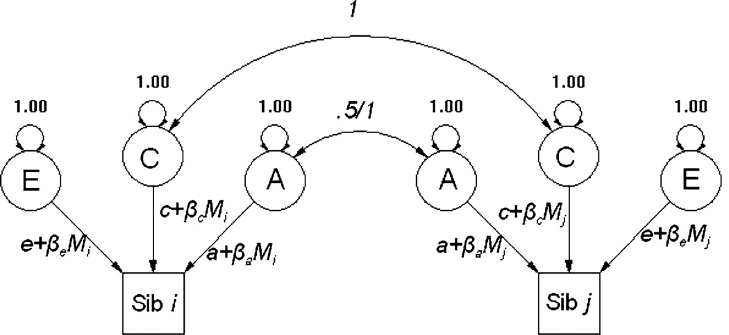
Following the publication of Purcell’s approach to the modeling of gene by environment interaction in 2002, many groups have implemented the analytic approaches detailed therein. This approach may more correctly be described as a flexible moderation framework, in which the moderator is the independent variable. Basically, Purcell’s approach allows interaction effects on all sources of variance (including common and unique environmental sources of variance) as opposed to being restricted to moderating the genetic sources of variance. To summarize, as shown in Fig. 1, the approach incorporates linear regressions on the path coefficients, in effect further partitioning the variance into that which is unrelated to the moderator (an intercept within a standard regression model) and that which is associated with the moderator (the slope or beta parameter).

Fig. 1.

Path diagram for the Purcell moderator model

This modeling approach was specifically designed for situations in which both the independent and dependent variables are continuous. To this end, Purcell (2002) strongly advocated reporting the unstandardized results, because although standardizing the solution could provide information regarding the relative values of the variance components for a given value of the moderator, much information regarding the source of the changes in variance is lost. While reporting the unstandardized estimates provides a simple solution in the case of a continuous dependent variable, this situation is largely untenable for ordinal and binary data, as the liability threshold model requires a variance constraint to allow identification. The purpose of the current paper is to present solutions for use with polychotomous (in which there are more than two categories) and binary data.

The problem of ordinal data

When working with a continuous dependent variable, collected from siblings or twin pairs, structural equation modeling analyses fit the means and covariance predicted by the model to those same statistics in the data. However, when working with univariate ordinal data from pairs of twins or siblings the data consist of a bivariate contingency table with c² cells (where c is equal to the number of categories). It is important to note, that for a variable to be considered ordinal, the categories within the data must be arranged in a meaningful ordered sequence. Categorical data, such as favorite sport or food, in which no meaningful order exists, may be analyzed as a series of binary dummy variables.

Behavioral genetic analyses of ordinal data usually adopt a threshold model approach, describing discrete traits as reflecting an underlying normal distribution of liability (the vulnerability, susceptibility, or predisposition) that has not been, or cannot be, measured directly or with sufficient precision. Instead, liability is measured as a series of ordered categories, characterized by phenotypic discontinuities that occur when the liability reaches a given threshold. Liability is assumed to reflect the combined effects of a large number of genes and environmental factors each of small effect, also known as the multifactorial model (Neale and Cardon 1992). Under these conditions the expected proportion of pairs in cell ij is (Neale et al. 1994):

$$P_{ij}={\int }_{t_{i-1}}^{t_i}{\int }_{t_{j-1}}^{t_j}\varphi (x_1,x_2)\mathrm{d}{x}_2\mathrm{d}{x}_1$$ (1)

where ti and tj refer to the thresholds of the first and second twins, respectively; t₀ = −∞; t_c = ∞; and φ(x₁, x₂) is the bivariate normal density function (Neale et al. 1994):

$$|2\pi \Sigma {|}^{-n/2}\text{exp}\{-\frac{1}{2}(x_k-{\mu }_k)\prime {\Sigma }^{-1}(x_k-{\mu }_k)\}$$ (2)

in which Σ is the population variance–covariance matrix, x_k is the (column) vector of observed data from family k and μ _k is the vector of population means. However, as the measurement scale of liability is unknown, there is no information regarding the population mean and variance. Thus to ensure the identification of the model parameters the liability distribution is assumed to be standard normal with a mean of zero and a variance of one. In practice this restriction is imposed by constraining the estimated variance of ordinal variables to unity, which maps the thresholds on a z scale. An alternative approach in the context of general mixed models is to constrain the variance of one of the sources, e.g., the unique environmental variance to unit (Boomsma et al. 2008).

While these approaches work admirably in most situations, a consequence of these constraints is that the resulting estimates are always standardized. Quite simply as traditionally conceptualized under a liability threshold model, there is insufficient information to investigate the change in the absolute magnitude of the genetic and environmental variances when analyzing ordinal data. However a recent re-parameterization of the threshold model by Mehta et al. (2004) provides a solution to this problem when working with polychotomous data.

A solution for the polychotimous case

Mehta et al. (2004) demonstrated that interval level information (means and variances) can be estimated from ordinal level information. In essence, the scale of the latent liability distribution is arbitrary. Thus, fixing any two thresholds will identify the latent distribution on an arbitrary scale. That is, the distance between adjacent thresholds can be parameterized to estimate the mean and the variance of the scale of measurement.

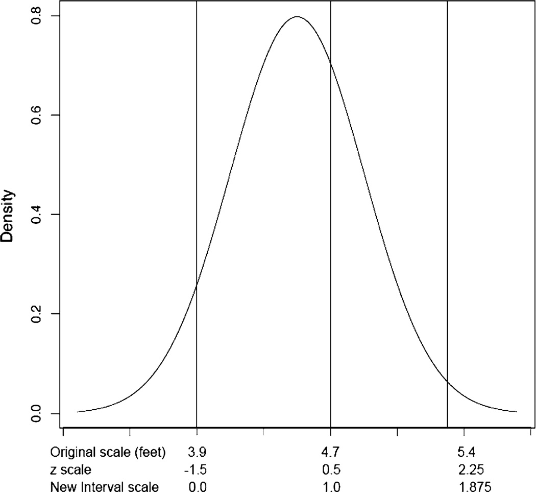
Consider their example of height measured in feet, in which the mean in a sample of children was 4.5 with a standard deviation of 0.4. If we imagine that this variable had been collected as (or transformed into) a categorical variable with the cut points illustrated in Fig. 2, using the liability threshold model we could map the underlying latent height distribution to a standard normal and estimate the thresholds, in z score units (z), as −1.5, 0.5 and 2.25. If we knew the true cut points we could fix the thresholds to these values and recover the original distribution. However, in practice the true distribution of liability is unmeasured, but if we fix the first two thresholds, in this case to 0 and 1, the means and standard deviations for the underlying liability variable can be recovered on a new arbitrary scale.

Fig. 2.

Height in a sample of children, thresholds are shown in feet, z units and the new interval scale units

Following Mehta et al. the standard deviation of height in the new units (u) can be calculated as:

$$\mathrm{S}\mathrm{D}({\text{height}}^u)=\frac{{\tau }_2^u-{\tau }_1^u}{{\tau }_2^z-{\tau }_1^z}=\frac{1-0}{0.5-(-1.5)}=\frac{1}{2}=0.5,$$

where τ represents the threshold on either the new (u) or z scales. Correspondingly, the mean can be calculated as:

$$E({\text{height}}^u)={\tau }_1^u-{\tau }_1^z\times \mathrm{S}\mathrm{D}({\text{height}}^u)=0-(-1.5)\times 0.5=0.75$$

While the third threshold (and any subsequent thresholds) can be recovered from:

$${\tau }_3^u=E({\text{height}}^u)+{\tau }_3^z\times \mathrm{S}\mathrm{D}({\text{height}}^u)=0.75+2.25\times 0.5=1.875.$$

The implementation of this method within Mx involves explicitly modeling the relationship between the liability threshold model and the interval level information. It is important to note that fixing the first two thresholds to the same values (0 and 1) for all family members does not imply that a single mean and standard deviation are sufficient to summarize the data. Differences in the thresholds between first and second born twins on the z scale will result in birth order differences in the standard deviations, and by extension, the means on the new scales. Thus, fixing the first two thresholds for all individuals effectively allows test of equality of means and standard deviations between first and second born twins or between twins and singleton siblings.

To estimate a polychoric correlation under the traditional liability threshold model, for a trait with three categories in pairs of siblings (s₁ and s₂), the threshold and covariance matrices Z and C are defined as: $Z=\left[\begin{array}{cc}\hfill {\tau }_{11}^z\hfill & \hfill {\tau }_{12}^z\hfill \\ \hfill {\tau }_{21}^z\hfill & \hfill {\tau }_{22}^z\hfill \\ \hfill {\tau }_{31}^z\hfill & \hfill {\tau }_{32}^z\hfill \end{array}\right]$, and $C=\left[\begin{array}{cc}\hfill 1\hfill & \hfill r(s_1,s_2)\hfill \\ \hfill r(s_1,s_2)\hfill & \hfill 1\hfill \end{array}\right]$, where r(s₁, s₂) is the polychoric correlation of the trait between the siblings. In Mx code these matrices can be declared as:

Z Full 3 2
C Stan 2 2

and provided using the following:

Threshold Z;
Covariance C;

Under the new interval liability model, the Z and C matrices are defined as: $Z=\left[\begin{array}{cc}\hfill {\tau }_{11}^z\hfill & \hfill {\tau }_{12}^z\hfill \\ \hfill {\tau }_{21}^z\hfill & \hfill {\tau }_{22}^z\hfill \\ \hfill {\tau }_{31}^z\hfill & \hfill {\tau }_{32}^z\hfill \end{array}\right]=\left[\begin{array}{cc}\hfill 0\hfill & \hfill 0\hfill \\ \hfill 1\hfill & \hfill 1\hfill \\ \hfill {\tau }_{31}^u\hfill & \hfill {\tau }_{32}^u\hfill \end{array}\right]-\left[\begin{array}{cc}\hfill E(s_1^u)\hfill & \hfill E(s_2^u)\hfill \\ \hfill E(s_1^u)\hfill & \hfill E(s_2^u)\hfill \\ \hfill E(s_1^u)\hfill & \hfill E(s_2^u)\hfill \end{array}\right]÷\left[\begin{array}{cc}\hfill \mathrm{S}\mathrm{D}(s_1^u)\hfill & \hfill \mathrm{S}\mathrm{D}(s_2^u)\hfill \\ \hfill \mathrm{S}\mathrm{D}(s_1^u)\hfill & \hfill \mathrm{S}\mathrm{D}(s_2^u)\hfill \\ \hfill \mathrm{S}\mathrm{D}(s_1^u)\hfill & \hfill \mathrm{S}\mathrm{D}(s_2^u)\hfill \end{array}\right]$, and $C=\left[\begin{array}{cc}\hfill 1\hfill & \hfill r(s_1,s_2)\hfill \\ \hfill r(s_1,s_2)\hfill & \hfill 1\hfill \end{array}\right]=\left[\begin{array}{cc}\hfill 1/\mathrm{S}\mathrm{D}(s_1^u)\hfill & \hfill \hfill \\ \hfill \hfill & \hfill 1/\mathrm{S}\mathrm{D}(s_2^u)\hfill \end{array}\right]\times \left[\begin{array}{cc}\hfill V(s_1^u)\hfill & \hfill C(s_1^u,s_2^u)\hfill \\ \hfill C(s_1^u,s_2^u)\hfill & \hfill V(s_2^u)\hfill \end{array}\right]\times \left[\begin{array}{cc}\hfill 1/\mathrm{S}\mathrm{D}(s_1^u)\hfill & \hfill \hfill \\ \hfill \hfill & \hfill 1/\mathrm{S}\mathrm{D}(s_2^u)\hfill \end{array}\right]$

In Mx code these matrices can be provided using the following:

Threshold Z;
Covariance C;

where:

T Full 3 2 ! contains the new threshold matrix
S Sym 2 2 ! contains the model implied covariance structure
M Full 1 2 ! contains the means matrix
U Unit 2 1 ! contains a vector (# rows = the number of individuals) of 1 s the
! purpose of which is to duplicate the standard deviation matrix
X Unit 3 1 ! contains a vector (# rows = the number of thresholds) of 1 s the
!purpose of which is to duplicate the means matrix

and

• Z = (T − X@M)%(X@\SQRT(\D2V(S)));

• D = \V2D(U%\SQRT(\D2V(S)));

• C = D × S × D;

where (X@M)produces a full matrix [3, 2] containing the means on the new scale and (X@\SQRT(\D2V(S))) produces a full matrix [2, 2] containing the standard deviations on the new scale and, \V2D(U%\SQRT(\D2V(S)))produces a diagonal matrix [2, 2] containing the inverse of the standard deviations on the new scale. Following this the extension to the moderated regression case involves an expansion of the S matrix from a simple polychoric correlation to the variance–covariance model summarized in Fig. 1. It is usually necessary to bound the thresholds ${\tau }_{31}^u$ and ${\tau }_{32}^u$ to be greater than 1, in order to avoid computing negative likelihoods (and hence incomputable log-likelihoods) with Eq. 1. A more general technique when there are more than two categories is to pre-multiply the matrix T with a lower triangular matrix L, which has every element on and below the diagonal fixed to one, and every element above the diagonal fixed to zero. The elements of T are then estimated deviations from the preceding threshold and all free elements in the T matrix are bounded to be strictly greater than zero.

Towards a solution for binary data

Unfortunately, the interval liability approach requires at least three ordered categories to extract interval level information. Despite this limitation, a number of analytic options are available to try and recover both the standardized and absolute path coefficients when working with binary data. Obviously the total variance of the trait could be constrained to unity across all values of the moderator. However, to the extent that the moderation is expected to lead to changes in the total magnitude of the variance, this approach is obviously undesirable and is unlikely to recover the absolute variance coefficients. A conceptually attractive approach would be to apply the continuous model to the binary data, simply substituting a threshold model for the means model. However, this model is not identified without additional constraints. Similarly, analyzing the binary data using a model for continuous data also seems attractive. However, this approach invalidates the likelihood ratio tests of hypotheses and may bias parameter estimates. The solution we propose is to use a constrained binary model in which the variance is constrained to unity at a specified value of the moderator.

Simulations

To determine the extent to which the constrained binary and Mehta et al. approaches recovered the information contained in the continuous liability distribution, we simulated data under three sets of parameters (summarized in Table 1) and examined the estimated absolute and standardized variance components produced by each approach. All simulations included a small mean effect of the moderator, β = .05.

Table 1.

Additive genetic (A) common environmental (C) and unique environmental (E) unmoderated variance components and moderator betas

	Simulation 1		Simulation 2		Simulation 3
	VC	β	VC	β	VC	β
A	.3	.45	3	.71	5	.71
C	.2	0	.5	.45	1	.32
E	.2	.32	4	1	4	.63

One hundred replicate samples of 5,000 monozygotic and 5,000 dizygotic twin pairs were simulated under each set of parameters. The moderator variables for each twin were randomly sampled from the unit normal distribution, and were not correlated between members of the twin pair. The use of standardized moderators avoids computation problems that may arise through correlation of the main and interaction effects, and increases the interpretability of the results (Aiken and West 1991). In each case a continuous data set was simulated. To create a binary phenotype a single threshold was then applied, the lower 20% were recoded as one with the remainder recoded zero. To create an ordinal phenotype thresholds were applied at −1 and 1, scores less than −1 were recoded as zero, scores between −1 and 1 (inclusive) were recoded as one, while scores greater than one were recoded as two. This resulted in symmetric categories with 75% of the sample falling in the middle category in simulation 1, 30% in simulation 2 and 20% in simulation 3.

We analyzed the binary data using the constrained binary model and the ordinal data using the Mehta et al. approach described above. For the binary case the variance was constrained to unit at the mean of the moderator (0). In addition, the continuous data (from which the binary and ordinal data arose) were also analyzed using a standard moderated regression script for continuous data (after Purcell 2002). As recommended by Purcell all analyses included a simple regression of the moderator on the mean/threshold model, which accounted for the mean effect so that the decomposition of variance was not influenced by this effect. Example scripts for the ordinal and constrained binary analysis are given in Appendix 1 and 2.

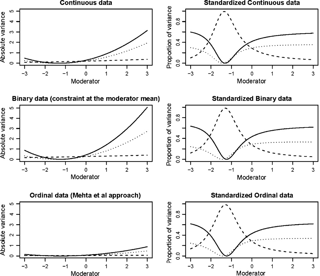
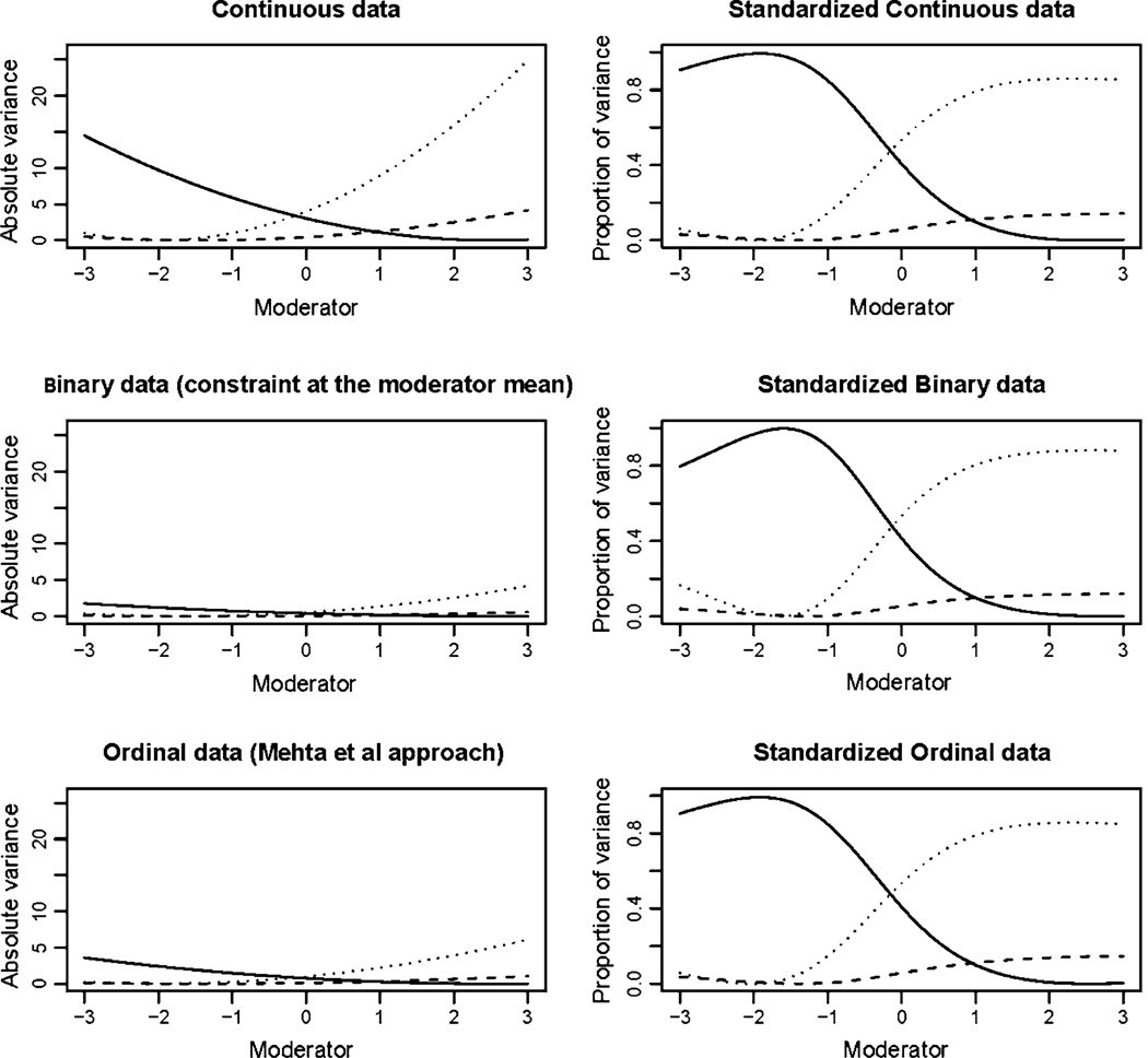
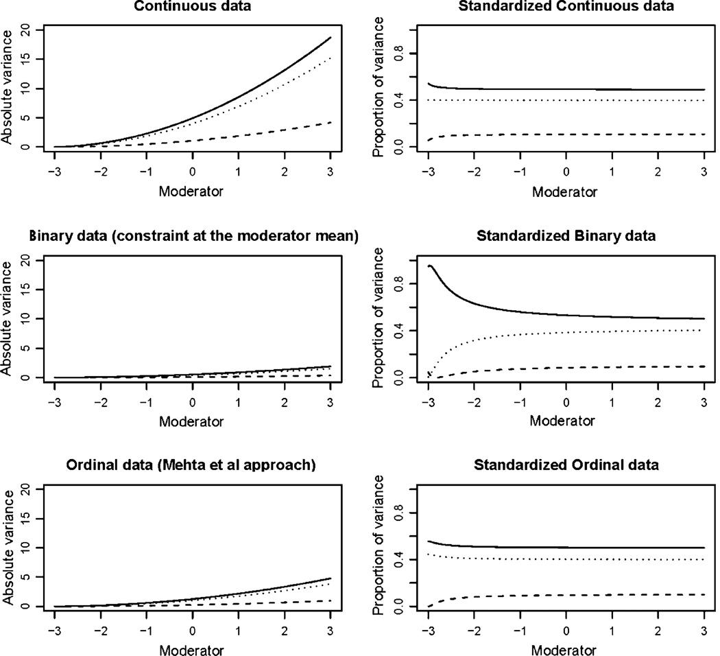
In the first two simulations, analysis of the continuous data performed well returning the simulation parameters. Across simulations, comparison of the continuous, binary and ordinal data reveals that the binary and ordinal analyses adequately reproduce the A × E_E effects present in the data. As may be expected, the scales of the unstandardized solutions (left column, Figs. 3, 4, and 5) differ markedly. Standardization removes this difference and assuming that the moderator has been mean-centered prior to analysis, allows a direct comparison between the values obtained from a constrained binary or ordinal analysis and those from a standard ACE or ADE analysis.

Fig. 3.

Results from simulation 1: additive genetic variance is indicated by the solid line, common environment as a broken line and unique environment by the dotted line. Absolute variance is shown in the left column with standardized proportions in the right column. The analysis of the continuous trait simulated prior to imposing the binary threshold is shown on the top row. The second row shows the results under a threshold model where the variance was constrained to equal one at the mean of the moderator (0). The third row shows the results obtained from the analysis of the ordinal data using the Mehta et al. approach

Fig. 4.

Results from simulation 2: additive genetic variance is indicated by the solid line, common environment as a broken line and unique environment by the dotted line. Absolute variance is shown in the left column with standardized proportions in the right column. The analysis of the continuous trait simulated prior to imposing the binary threshold is shown on the top row. The second row shows the results under a threshold model where the variance was constrained to equal one at the mean of the moderator (0). The third row shows the results obtained from the analysis of the ordinal data using the Mehta et al. approach

Fig. 5.

Results from simulation 3: additive genetic variance is indicated by the solid line, common environment as a broken line and unique environment by the dotted line. Absolute variance is shown in the left column with standardized proportions in the right column. The analysis of the continuous trait simulated prior to imposing the binary threshold is shown on the top row. The second row shows the results under a threshold model where the variance was constrained to equal one at the mean of the moderator (0). The third row shows the results obtained from the analysis of the ordinal data using the Mehta et al. approach

A small bias was observed in results of the continuous data analysis of simulation 3. In the graph showing the standardized results the estimates fan out as the total variance approaches zero. In the absence of bias this graph would be characterized by three parallel lines. The results from the ordinal data analysis showed a similar degree of bias, while the bias was exaggerated in the constrained binary model as the value of the moderator decreased (Fig. 5). However, it should be noted that this was a highly contrived example, which was deliberately chosen to provoke optimization difficulties. In this simulation the moderating effects were proportionate to the un-moderated variance components and the region in which the bias was most extreme was populated by less than 5% of the sample. By comparison, no such bias was observed in simulation 1 where the variance approached zero in a more densely populated area of the data, suggesting that the bias in simulation 3 results from a combination of low variance and sparse data rather than the low variance per se.

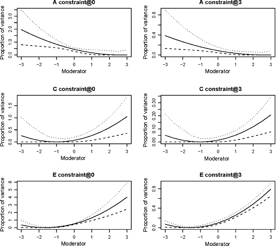
To investigate the influence of the specification of the constraint in the binary model we simulated additional binary data under the parameters used for simulation 2. For this simulation we analyzed each data set twice with the total variance constrained to unity at the mean of the moderator variable, 0, and at an extreme value of the moderator, 3. As shown in Fig. 6, while specification of the constraint does have a substantial influence on the scale on which the results are mapped, the effects on the point estimates were negligible (shown using an unbroken line). In addition to examining the point estimates we also computed confidence intervals by calculating the point estimates for a range of moderator values and requesting confidence intervals on these computed estimates. There were subtle effects of constraint specification on the confidence intervals (shown in Fig. 6 using dotted and dashed lines). These effects were most obvious when considering the unique environmental estimates. The confidence intervals were noticeably tighter near the value of the moderator at which the total variance was constrained to unity. However, this effect was not seen on the confidence intervals surrounding the standardized estimates. An additional simulation (not shown here) which included a quadratic moderator effect showed the same pattern of results.

Fig. 6.

Analysis of a representative data set showing the effects of constraint specification: The absolute point estimates are illustrated with the solid line, while the 95% confidence intervals are given by the dotted and dashed lines. The total variance was constrained to unity in at 0 (the mean of the moderator) in the left column and at three in the right column. Additive genetic estimates are shown on the top row, common environment in the middle row and unique environment on the bottom row. Note that the y axis differs between the left and right columns

Thus, while the specification of the constraint does not alter the pattern of the point estimates it can affect confidence intervals. We would strongly recommend standardizing the moderator and placing the constraint at the mean of the transformed moderator. This solution is intuitively attractive in that the tightest possible confidence intervals are observed in the region with the most data. In addition, this strategy also aids in the interpretation of results by placing the estimates for the mean of the sample on the same scale as those from an unmoderated analysis.

In conclusion, these simulations have shown that while it is possible to recover unbiased estimates of G × E effects from binary and ordinal data their scale depends on the location of the variance constraint in the case of the binary data, and the fixed values of the thresholds in the ordinal case. There is insufficient information in either the ordinal or the binary case, to recover the true distribution of liability. However, as transformation and re-scaling are common practices when working with continuous data, characterizing the observed interaction is arguably more important for the interpretation and implications of the analysis than the scale on which the variable is analyzed or graphed. Thus, we would suggest that Purcell’s G × E approach is suitable for use with ordinal or binary data with minimal modification of the existing Mx scripts. In common with the approach described by Purcell, the approach described here is suitable only for E_C and E_E type moderator variables that are otherwise independent of the outcome variable. Unchangeable variables, such as age, genotype and chromosomal sex are the most suitable for this type of analysis; more complex methods are required when G × E is accompanied by G–E covariance.

Appendix 1

Example Mx script for a generalized moderated regression model with the ordinal data using the interval liability model

G1: Parameters
#define ndef 1 ! n definition variables: sex moderator1
#define nmod 2 ! unmod, moderator1
#define nind 2 ! n individuals in largest sibship
#define nthr 2 ! number of thresholds 2 = 3 categories
Data Calc NGroups = 3
Begin Matrices;
A full 1 nmod free
C full 1 nmod free
E full 1 nmod free
M full 1 nind free ! mean
B full 1 ndef free ! effects of covariates on the mean
H unit nind nind ! mz constants
J stand nind nind ! dz constants
R ident nind nind
T Full nthr nind ! contains the new threshold matrix
U unit nind 1
X Unit nthr 1 ! contains a vector of 1s
End Matrices;
Value .5 J 2 1
eq m 1 1 1 m 1 1 2
ma t
0 0
1 1
!starting values for A C and E
!unmoderated and moderated parameter start values
MATRIX A −.5 .5
MATRIX C .2 .2
MATRIX E .3 .1
labels coloumn A unmod mod
labels coloumn C unmod mod
labels coloumn E unmod mod
labels coloumn b mod
Options RSiduals
End
G2: MZ
DATA NINPUT = 8
labels rep zyg mod1 mod2 c1 c2 tw1 tw2
Ord File = mz1
select mod1 mod2 tw1 tw2;
Definition_variables mod1 mod2;
Matrices = Group 1
V full nmod nind ! contains coefficients of the cov corrections
W full ndef nind ! contains covariates for means regression
End Matrices;
SP V 0 0 mod1 mod2;
VALUE 1 V 1 1 V 1 2
! contains 1 s for unmoderated cov elements and covariates for moderated
! cov elements
SP W mod1 mod2;
! contains covariates for means regression
Begin Algebra;
S=
(H.((U@A)*V).(V′*(U@A)′)) + !variance/cov due to A
((U@C)*V).(V′*(U@C)′) + !variance/cov due to C
(R.((U@E)*V).(V′*(U@E)′)); !variance/cov due to E
Z = (T − X@(M + (B*W)))%(X@\SQRT(\D2V(S)));
D = \V2D(U′%\SQRT(\D2V(S)));
End Algebra;
Threshold Z;
Covariance D*S*D;
End
G3: DZ
DATA NINPUT = 8
labels rep zyg mod1 mod2 c1 c2 tw1 tw2
ord File = dz1
select mod1 mod2 tw1 tw2;
Definition_variables mod1 mod2;
Matrices = Group 1
V full nmod nind
W full ndef nind
End Matrices;
SP V 0 0 mod1 mod2;
SP W mod1 mod2;
VALUE 1 V 1 1 V 1 2
Begin Algebra;
S=
(J.((U@A)*V).(V′*(U@A)′)) + !variance/cov due to A
((U@C)*V).(V′*(U@C)′) + ! variance/cov due to C
(R.((U@E)*V).(V′*(U@E)′)); ! variance/cov due to E
Z = (T−X@(M + (B*W)))%(X@\SQRT(\D2V(S)));
D = \V2D(U′%\SQRT(\D2V(S)));
End Algebra;
Threshold Z;
Covariance D*S*D;
End

Appendix 2

Example Mx script for a generalized moderated regression model with the binary data using a variance constraint at a specified value of the moderator

!Constrained binary script
#define ndef 1 ! n definition variables: sex moderator1
#define nmod 2 ! unmod, moderator1
#define nind 2 ! n individuals in largest sibship
G!: Parameters
Data Calc NGroups = 4
Begin Matrices;
A full 1 nmod free
C full 1 nmod free
E full 1 nmod free
M full 1 nind free ! threshold
B full 1 ndef free ! mean effects
H unit nind nind ! mz constants
J stand nind nind ! dz constants
U unit nind 1
D ident nind nind
End Matrices;
Value .5 J 2 1
!starting values for threshold
MATRIX M .8 .8
!starting values for beta
MATRIX B 0.05
!starting values for A C and E
!unmoderated and moderated parameter start values
MATRIX A 1.5 − .5
MATRIX C .7 .4
MATRIX E 2 1
labels coloumn A unmod mod
labels coloumn C unmod mod
labels coloumn E unmod mod
labels coloumn b mod
Options RSiduals
End
G2: MZ
DATA NINPUT = 10
labels loop zyg mod1 mod2 mod1b mod2b tw1 tw2
bintw1 bintw2
Ord File = mz1
select mod1 mod2 bintw1 bintw2;
Definition_variables mod1 mod2;
Matrices = Group 1
V full nmod nind ! contains coefficients of the cov corrections
W full ndef nind ! contains covariates for threshold regression
End Matrices;
SP V 0 0 mod1 mod2;
VALUE 1 V 1 1 V 1 2
! contains 1 s for unmoderated cov elements and covariates for moderated
! cov elements
SP W mod1 mod2;
! contains covariates for thresholds regression
Thresholds M + B*W;
Covariance
(H.((U@A)*V).(V′*(U@A)′))+
((U@C)*V).(V′*(U@C)′)+
(D.((U@E)*V).(V′*(U@E)′));
End
G3: DZ
DATA NINPUT = 10
labels loop zyg mod1 mod2 mod1b mod2b tw1 tw2
bintw1 bintw2
Ord File = dz1
select mod1 mod2 bintw1 bintw2;
Definition_variables mod1 mod2;
Matrices = Group 1
V full nmod nind
W full ndef nind
End Matrices;
SP V 0 0 mod1 mod2;
SP W mod1 mod2;
VALUE 1 V 1 1 V 1 2
Thresholds M + B*W;
Covariance
(J.((U@A)*V).(V′*(U@A)′))+
((U@C)*V).(V′*(U@C)′)+
(D.((U@E)*V).(V′*(U@E)′));
End
Constraint group to force variance = 1 when moderator is zero
constraint
begin matrices;
A full 1 1 free
C full 1 1 free
E full 1 1 free
F full 1 1 free
G full 1 1 free
H full 1 1 free
M full 1 1 fixed !moderator
U unit 1 1
End matrices;
EQ A 1 1 1 A 4 1 1
EQ C 1 1 1 C 4 1 1
EQ E 1 1 1 E 4 1 1
EQ A 1 1 2 F 4 1 1
EQ C 1 1 2 G 4 1 1
EQ E 1 1 2 H 4 1 1
MATRIX m 0 !value of the moderator for constraint begin Algebra;
T=
((A + (F*M))*(A + (F*M)))+
((C + (G*M))*(C + (G*M)))+
((E + (H*M))*(E + (H*M)));
end algebra;
Contrain U = T;
option jiggle append
End

References

- Aiken LS, West SG. Multiple regression: testing and interpreting interactions. Thousand Oaks: Sage; 1991. [Google Scholar]
- Boomsma DI, van Someren EJ, Beem AL, de Geus EJ, Willemsen G. Sleep during a regular week night: a twin-sibling study. Twin Res Hum Genet. 2008;11(5):538–545. doi: 10.1375/twin.11.5.538. [DOI] [PubMed] [Google Scholar]
- Eaves LJ, Last K, Martin NG, Jinks JL. A progressive approach to non-additivity and genotype-environmental covariance in the analysis of human differences. Br J Math Stat Psychol. 1977;30:1–42. [Google Scholar]
- Mather K, Jinks JL. Introduction to biometrical genetics. Ithaca: Cornell University Press; 1977. [Google Scholar]
- Mehta PD, Neale MC, Flay BR. Squeezing interval change from ordinal panel data: latent growth curves with ordinal outcomes. Psychol Methods. 2004;9(3):301–333. doi: 10.1037/1082-989X.9.3.301. [DOI] [PubMed] [Google Scholar]
- Neale MC, Cardon LR. Methodology for genetic studies of twins and families. Dordrecht: Kluwer Academic Publishers; 1992. [Google Scholar]
- Neale MC, Eaves LJ, Kendler KS. The power of the classical twin study to resolve variation in threshold traits. Behav Genet. 1994;24(3):239–258. doi: 10.1007/BF01067191. [DOI] [PubMed] [Google Scholar]
- Purcell S. Variance components models for gene–environment interaction in twin analysis. Twin Res. 2002;5:554–571. doi: 10.1375/136905202762342026. [DOI] [PubMed] [Google Scholar]