Bayesian Longitudinal Plateau Model of Adult Grip Strength

Abstract

Objectives

This article illustrates the use of applied Bayesian statistical methods in modeling the trajectory of adult grip strength and in evaluating potential risk factors that may influence that trajectory.

Methods

The data consist of from 1 to 11 repeated grip strength measurements from each of 498 men and 533 women age 18–96 years in the Fels Longitudinal Study (Roche AF. 1992. Growth, maturation and body composition: the Fels longitudinal study 1929–1991. Cambridge: Cambridge University Press). In this analysis, the Bayesian framework was particularly useful for fitting a nonlinear mixed effects plateau model with two unknown change points and for the joint modeling of a time-varying covariate. Multiple imputation (MI) was used to handle missing values with posterior inferences appropriately adjusted to account for between-imputation variability.

Results

On average, men and women attain peak grip strength at the same age (36 years), women begin to decline in grip strength sooner (age 50 years for women and 56 years for men), and men lose grip strength at a faster rate relative to their peak; there is an increasing secular trend in peak grip strength that is not attributable to concurrent secular trends in body size, and the grip strength trajectory varies with birth weight (men only), smoking (men only), alcohol consumption (men and women), and sports activity (women only).

Conclusions

Longitudinal data analysis requires handling not only serial correlation but often also time-varying covariates, missing data, and unknown change points. Bayesian methods, combined with MI, are useful in handling these issues.

The goal of this article is to illustrate the application of Bayesian statistical methods in fitting a longitudinal model with multiple unknown change points, time-varying covariates, and missing data, in the context of an analysis of adult grip strength using data from the Fels Longitudinal Study (Roche, 1992). Low muscle strength is related to frailty in later life. A faster rate of increase in muscle strength early in life, higher peak strength, and a slower rate of decline with aging can prevent or delay the onset of sarcopenia (agerelated decline in muscle mass and strength) (Rolland et al., 2008; Yliharsila et al., 2007). Other studies have examined the adult muscle strength trajectory using serial data (Frederiksen et al., 2006; Harris, 1997; Kallman et al., 1990). The purposes of this analysis, however, are not only to (i) investigate the longitudinal pattern of change in dominant hand grip strength (a measure of muscle strength) during adulthood, by sex, controlling for body size and secular trends but also to (ii) assess the significance of associations between that pattern and the following risk factors: birth weight, infant growth rate, sports activity, smoking (ever and current), and alcohol consumption (ever, current, and current amount). We seek to determine which of these risk factors are significantly associated with the rate of change in grip strength during early adulthood, with peak grip strength, and with the rate of change in grip strength during old age. Birth weight and early growth rate are included as risk factors representing early life events, which might impact adult muscle strength (Inskip et al., 2007; Kuh et al., 2002). The remaining candidate risk factors represent lifestyle factors that might impact muscle strength (Harris, 1997).

GRIP STRENGTH DATA FROM THE FELS LONGITUDINAL STUDY

The Fels Longitudinal Study, which began in southwestern Ohio in 1929, is the world's longest ongoing longitudinal study of human growth, development, and body composition changes over the lifespan (Roche, 1992). The data analyzed herein consist of serial dominant hand grip strength measurements collected between 1985 and 2008 from 498 men and 533 women (age 18–96 years, born 1905–1989) participating in the Fels Longitudinal Study. Participants were grouped into six birth cohorts by decade (pre-1940, 1940–1949, 1950–1959, 1960–1969, 1970–1979, and 1980–1989) to adjust for secular trends. Participants born before 1930 were grouped together with those born in 1930–1939 because of the small number of participants born in any single earlier decade. Each participant had from 1 to 11 visits (median = 3) since 1985 for a total of 4,045 visits. See Table 1 for sample sizes by sex and birth cohort.

TABLE 1.

Sample size by sex and birth cohort

	Males			Females
Birth cohort	Age range (years)	Subjects	Visits	Age range (years)	Subjects	Visits
1905–1939	46–96	86	347	46–92	100	409
1940–1949	36–68	83	352	36–68	86	422
1950–1959	25–58	101	381	25–58	102	424
1960–1969	18–47	88	331	18–48	104	439
1970–1979	18–38	86	331	18–38	78	316
1980–1989	18–27	54	139	18–26	63	154
Total	18–96	498	1,881	18–92	533	2,164

Grip strength for the self-reported dominant hand was first measured in the Fels Longitudinal Study in 1985 using a Lafayette Hand Dynamometer (Model 78010, Lafayette Instrument Company, Lafayette, IN). After 2003, a JAMAR Hydraulic Hand Dynamometer (Model 5030J1, JLW Instruments, Chicago, IL) was used. As grip strength measured by these two devices is not exactly equivalent; we rescaled the older Lafayette measurements using an orthogonal distance regression (Fuller, 1987) based on the data from 25 adults measured with both instruments at the same visit (JAMAR grip strength = 0.983 × Lafayette grip strength (kg) + 3.214 kg). Body weight (kg) and stature (cm) were measured according to standard anthropometric methods (Lohman et al., 1988). Body weight was recorded to the nearest 0.1 kg without shoes or any heavy clothing, and stature was measured to the nearest 0.1 cm without shoes. BMI (kg/m²) was then derived from body weight and stature. Birth weight (kg) was obtained from birth records. Many of these adult participants were observed during infancy, and two early growth rates (kg/year) were computed as the change in weight from birth to age 12 months and the annualized change from birth to age 2 years. Sports activity was self-reported on a scale of 1–5 using a Baecke Habitual Physical Activity questionnaire (Baecke et al., 1982). Both “ever” and “current” smoking and alcohol consumption status (0/1) were obtained from self-report, as was current alcohol consumption (categorized as none, occasionally, in moderation, or above moderation, where we defined “moderation” as one drink per day for women and two drinks per day for men and a “drink” as 12 oz. of beer, 4 oz. of wine, 1 oz. of hard liquor, or a single mixed drink). Signed informed consent was obtained from all participants. All protocols and procedures were approved by the Wright State University Institutional Review Board.

PLATEAU MODEL WITH UNKNOWN CHANGE POINTS

The term “plateau model” refers here to a piecewise linear model with a middle piece constrained to be flat. This model can be written as

$$y_{ij}=({\beta }_{\mathrm{L}}+b_{\mathrm{Li}})\text{min}(0,{\text{age}}_{ij}-t_1)+(\beta +b_i)+({\beta }_{\mathrm{U}}+b_{\mathrm{Ui}})\text{max}(0,{\text{age}}_{ij}-t_2){\epsilon }_{ij},$$ (1)

where y_ij is the dominant hand grip strength measurement for the ith subject's jth observation time, t₁ ≤ t₂ are the two unknown change points, β_L (the “lower slope”) represents the population-average rate of change in grip strength from age 18 years to t₁, β represents the population-average peak grip strength (from age t₁ to t₂), β_U (the “upper slope”) represents the population-average rate of change after age t₂, b_Li and b_Ui are random subject-specific deviations from the population-average slopes β_L and β_U, respectively, b_i is a random subject-specific deviation from the population-average peak grip strength β, and ε_ij are independent random errors distributed as N(0, σ²). In principle, it is possible to include random subject-specific deviations from the change points t₁ and t₂, cohort-specific change points, and/or cohort-specific lower and upper slopes; however, there was not enough information in our data to estimate these as evidenced by a lack of convergence of the fitting algorithm when attempting to do so.

In this model, serial correlation is modeled through random effects, with residuals assumed to be conditionally independent. As we only have grip strength data over a 23-year period, too few individuals have sufficient data both before t₁ and after t₂ to jointly estimate the random slopes. Thus, the potential correlation structures for the joint distribution of the three random effects are (i) b_Li, b_i and b_Ui independent, (ii) b_Li and b_i correlated and independent of b_Ui, and (iii) b_i and b_Ui correlated and independent of b_Li. The Gibbs sampling chains (see BAYESIAN JOINT MODEL FOR BMI AND GRIP STRENGTH below) only behaved well with structure (i).

Model (1) can also be written as

$$y_{ij}=\{\begin{array}{cc}(\beta +b_i)+({\beta }_{\mathrm{L}}+b_{\mathrm{Li}})({\text{age}}_{ij}-t_1)+{\epsilon }_{ij}\hfill & 18\le {\text{age}}_{ij}<t_1\hfill \\ (\beta +b_i)+{\epsilon }_{ij}\hfill & t_1\le {\text{age}}_{ij}\le t_2\hfill \\ (\beta +b_i)+({\beta }_{\mathrm{U}}+b_{\mathrm{Ui}})({\text{age}}_{ij}-t_2)+{\epsilon }_{ij}\hfill & t_2<{\text{age}}_{ij}.\hfill \end{array}\phantom{\}}$$

The locations where the plateau begins and ends, t₁ and t₂, are unknown, resulting in a model that is nonlinear in these parameters.

The plateau model was extended to include secular trends by allowing the peak grip strength to vary by birth cohort. The peak parameter β was replaced by β_k, where k indexes the six birth cohorts to produce cohort-specific estimates of peak grip strength. Figure 1 illustrates the fit to the data for males and females and demonstrates the presence of an increasing secular trend.

Fig. 1.

Grip strength vs. age trajectories, by sex (assuming BMI at age 45 is 25 kg/m², all continuous covariates at their sex-specific means, and all categorical covariates at their reference levels). The black lines represent estimated trajectories by birth cohort plotted over the range of ages observed for each cohort. From left to right, the lines are therefore in the birth cohort order 1980–1989 to 1905–1939.

WHY A PLATEAU MODEL?

The use of a plateau model was motivated by two facts. First, when doing exploratory plotting of the data, we fit smoothing splines to get an idea of what functional form would be appropriate for the grip strength trajectory. Ignoring secular trends, the curve appeared approximately quadratic. However, when fitting distinct curves to each cohort, it was clear that there was a secular trend and that, within cohort, the fit was approximately linear. No cohort was observed over the entire adult lifespan. Cohorts observed at younger ages had a positive slope, cohorts observed during middle age had a slope near zero, and cohorts observed at older ages had a negative slope. A plateau model with cohort-specific peak grip strength is consistent with these exploratory plots; that is, it allows the population mean grip strength to be constant over a period of time during middle adulthood. Second, the question that originally motivated this analysis was “What risk factors influence the rate of decline in old age?” and the plateau model provides a direct method of estimating the impact of each risk factor as a parameter of the model, namely as an interaction between the risk factor and the slope after the plateau.

TIME-VARYING COVARIATES

Adjusting for body size

To evaluate the association between risk factors and the grip strength trajectory, it is appropriate to adjust for body size. Body size was measured as stature (height) (HT, cm) and BMI = weight/stature² (kg/m²), with BMI log-transformed to achieve a more symmetric distribution and reduce the influence of values in the tail of the distribution on parameter estimation. Both stature and BMI change with age (Chumlea et al., 2009; Sorkin et al., 1999) so, if included in the model as covariates, these would be stochastic time-varying covariates. It is well documented that the inclusion of stochastic time-varying covariates in longitudinal data analysis requires care (Diggle et al., 2002; Fitzmaurice et al., 2004). One issue is the interpretation of model parameters. In a longitudinal model, each time-varying variable, including age (which is a nonstochastic time-varying variable—it changes systematically with time), has a between-individual effect and a within-individual effect. In our analysis, a between-individual effect represents the expected difference in grip strength between individuals with different values of the covariate (e.g., individuals with different HT), assuming all other covariates are equal (e.g., same age). A within-individual effect represents the expected change in grip strength associated with a within-individual change in the covariate (e.g., an increase in BMI), assuming all other covariates, including age, do not change. The problem is that the time-varying variable age cannot be held fixed when a covariate changes within an individual. Thus, the interpretation of the age-trajectory parameters and the effects of stochastic time-varying variables are confounded.

We prefer a model in which within-individual changes in grip strength over time are represented entirely by the parameters of the age effects; in our model, these are the lower and upper slopes. If we were to adjust for body size by including time-varying log(BMI) and HT, then the estimated lower and upper slopes would not represent the expected change in grip strength per year. To compute the expected change in grip strength per year in early adulthood, for example, one would have to sum the lower slope, the product of the expected change in log(BMI) per year and its parameter estimate [the estimated change in grip strength per unit change in log(BMI)], and the product of the expected change in HT per year and its parameter estimate. These expected changes in log(BMI) and HT are not predicted by the model and would have to be based on additional longitudinal modeling. An alternative is to adjust for body size by including time-invariant versions of log(BMI) and HT. This results in these covariates having only between-individual effects and the lower and upper slopes having the desired interpretation of the expected change in grip strength per year.

Restricting to between-individual effects

To remove the implication of within-individual effects for stature and BMI, we limited the effect of each to a between-individual effect by replacing each with a time-invariant within-individual summary. If the observation times were balanced in age, then this could have been done by using baseline values of stature and BMI, or stature and BMI at any commonly observed age. However, in many studies, including the Fels Longitudinal Study, individuals are observed at distinct times and often over nonoverlap-ping age ranges. Thus, baseline values, and also mean values, are not comparable for covariates that systematically change with age. As we have data from previous visits over the lifespan for these participants, we used maximum stature and an estimate of BMI at age 45 years (an arbitrarily chosen age—any age would do) to represent each individual's body size. The estimated BMI at age 45 years was obtained via a linear mixed model as shown in BAYESIAN JOINT MODEL FOR BMI AND GRIP STRENGTH below. Maximum stature and BMI at age 45 were estimated using all the data for each subject, not only visits since 1985 when grip strength measurements began.

Note that for the other time-varying variables included in our analysis (smoking, alcohol consumption, and sports activity), we do wish to imply that there are both between-and within-individual effects. Thus, these risk factors were not replaced by time-invariant summaries.

HANDLING MISSING UNBALANCED LONGITUDINAL DATA

An additional complication in any data analysis is missing data. Multiple imputation (MI) is a generally applicable method for handling missing data under the assumption of ignorability (Little and Rubin, 2002; Rubin, 1987). Methods exist for MI of balanced longitudinal data as a special case of multivariate missing data (Schafer, 1997). However, MI of unbalanced longitudinal data is more challenging. For our dataset, we have observations over such a large age range that any attempt to round off ages to try to create a balanced dataset for the purpose of MI is not feasible. Rounding off to the nearest year leads to very sparse data, and rounding off to a multiple of years leads to large numbers of individuals having more than one observation at the same rounded age. When no time-invariant covariates are missing, the multivariate linear mixed model can be used to impute unbalanced longitudinal data (Liu et al., 2000; Schafer and Yucel, 2002). In our analysis, however, there are missing time-invariant covariates (birth weight and two early growth rates).

The imputation method we used was an ad hoc method of resolving these difficulties. An imputation model is a model for prediction of missing data given observed data. The missing data in our case consist of both time-invariant and time-varying covariates. Let X represent the set of time-invariant covariates, Y represent the set of time-varying covariates, (X_mis, Y_mis) represent the missing data, and (X_obs, Y_obs) represent the observed (nonmissing) data. Then, the probability distribution function for the missing data given the observed data can be written as f(X_mis, Y_mis|X_obs, Y_obs) = f(X_mis|X_obs, Y_obs) × f(Y_mis|X_mis, X_obs, Y_obs). Thus, imputation can be performed in two stages with imputation models corresponding to these two factors. The difficulty is that, in the first stage, we need a model for time-invariant covariates given time-varying covariates. For balanced longitudinal data, this could be done by writing each time-varying variable as a set of variables, one for each observation time. For unbalanced longitudinal data, an approximation to this distribution is obtained by replacing each individual's time-varying covariate vector by a single summary (e.g., within-subject mean). Another difficulty is that, at the second stage, we have a model for longitudinal data and so must account for the serial correlation. As an approximation to the second stage of the model, we include these same summary values as additional covariates. In this way, each observation from an individual is modeled as correlated to this single summary value, thus inducing serial correlation in the imputation model.

Let Y* represent the within-individual summaries of the time-varying covariates. We approximate f(X_mis, Y_mis|X_obs, Y_obs) as f(X_mis|X_obs, Y*) × f(Y_mis|X_mis, X_obs, Y_obs, Y*), where X_mis in the second stage are the imputed values from the first stage. Thus, Stage 1 imputes for missing time-invariant covariates given observed time-invariant covariates and time-invariant summaries of the time-varying covariates, and Stage 2 imputes for missing time-varying covariates given observed and imputed time-invariant covariates, observed time-varying covariates, and time-invariant summaries of the time-varying covariates. Although admittedly ad hoc, this method has the advantage of being implementable with commonly available imputation routines for independent data such as SAS PROC MI (SAS, Cary, NC) or the aregImpute function in the R (R Development Core Team, 2009) library Hmisc (Harrell [with contributions from many other users], 2009). We used the default imputation method implemented by aregImpute, predictive mean matching, which uses a flexible additive model and handles both continuous and categorical variables (de Groot et al., 2008; Little and An, 2004; Siddique and Belin, 2008; van Buuren et al., 2006).

A straightforward time-invariant summary for a time-varying variable is its within-subject mean. However, as participants were observed over differing age ranges, these may not be comparable across participants. In this analysis, two time-invariant summaries for each longitudinal variable were included: the subject-specific means within each of two age ranges (<45 years and ≥45 years).

Specifically, the variables included in each stage of the imputation procedure model were as follows. The Stage 1 imputation was performed on a dataset with one record per individual. The time-invariant variables included in the model were birthday (years, e.g., 1/1/1960 = 1960.00), maximum stature, birth weight, infant growth rate from birth to age 1 year, and infant growth rate from birth to age 2 years. The summaries of time-varying variables included in the model were means before and after age 45 of the following variables: log(BMI), grip strength, smoking (ever and current), alcohol consumption (ever and current amount; current was excluded from the imputation as it can be derived from current amount), and sports activity. Stage 1 was performed separately for males and females.

For the Stage 2 imputation, we stratified by sex and by age group (age <45 years and age ≥45 years) because we did not want to assume that the relationships between variables were the same within these groups. Stage 2, for each stratum, was performed on a dataset with one record per observation time (multiple records per individual), and the model included the same time-invariant variables as in Stage 1 (with missing values for the k^th Stage 2 imputation replaced by imputed values from the k^th Stage 1 imputation), the time-varying variables age, log(BMI), grip strength, smoking (ever and current), alcohol consumption (ever and current amount), and sports activity, and, for each of these time-varying variables, the within-subject mean over the same age range as the stratum being imputed (age <45 years or age ≥45 years). For both the time-invariant variables and the within-subject means, each participant only has one value, and this value was replicated over all of that participant's observation times.

This two-stage imputation procedure was repeated five times to produce five complete datasets. The plateau model was then fit to each imputed dataset, and posterior inferences were pooled with appropriate corrections to account for between-imputation variability.

In the grip strength dataset, only 198 men and 207 women had at least one visit with nonmissing values for all the analysis variables (1,705 visits total). The variables missing most often were sport activity, birth weight, and early growth rate (see Table 2 and note that birth weight and early growth rate are time-invariant covariates; thus, their numbers of missing values represent participants rather than visits). Despite the large number of missing values for some covariates, using only five imputations led to relative efficiencies of at least 95% for all but one parameter in the final model and at least 99% for most. The one exception was the interaction between birth weight and peak grip strength for males, which had a relative efficiency of 91%.

TABLE 2.

Number (proportion) of missing values by variable

	Males		Females
Variable	Visits
Grip strength (kg)	48	(2.6%)	74	(3.4%)
BMI (kg/m2)	6	(0.3%)	8	(0.4%)
Sport activity index (1–5)	243	(12.9%)	272	(12.6%)
Has smoked (yes/no)	9	(0.5%)	9	(0.4%)
Currently smokes (yes/no)	17	(0.9%)	9	(0.4%)
Has drank alcohol (yes/no)	43	(2.3%)	37	(1.7%)
Currently drinks alcohol (yes/no)	66	(3.5%)	71	(3.3%)
Currently drinks alcohol (amount)	81	(4.3%)	78	(3.6%)
	Participants
Birth weight (kg)	184	(36.9%)	217	(40.7%)
Early growth rate (kg/year from 0 to 1 years)	280	(56.2%)	311	(58.3%)
Early growth rate (kg/year from 0 to 2 years)	274	(55.0%)	308	(57.8%)

BAYESIAN JOINT MODEL FOR BMI AND GRIP STRENGTH

The full specification of the Bayesian joint mixed model for BMI and grip strength is as follows. For males and females separately, the natural logarithm of BMI was modeled as a quadratic polynomial in age (centered at 45 years) with random effects and continuous interactions between birthday (years, centered at January 1, 1960) and each polynomial term. The random effects are modeled as multivariate normal with an unstructured covariance matrix. This model can be expressed as

$$\log \left({\text{BMI}}_{ij}\right)=[{\theta }_{1\mathrm{a}}+{\theta }_{1\mathrm{b}}({\text{birthday}}_i-1960)+{\eta }_{1\mathrm{i}}]+[{\theta }_{2\mathrm{a}}+{\theta }_{2\mathrm{b}}({\text{birthday}}_i-1960)+{\eta }_{2\mathrm{i}}]({\text{age}}_{ij}-45)+[{\theta }_{3\mathrm{a}}+{\theta }_{3\mathrm{b}}({\text{birthday}}_i-1960)+{\eta }_{3\mathrm{i}}]{({\text{age}}_{ij}-45)}^2+{\delta }_{ij}({\eta }_{1\mathrm{i}},{\eta }_{2\mathrm{i}},{\eta }_{3\mathrm{i}})~\text{MVN}(0,\mathrm{S}){\delta }_{ij}\text{i.i.d.}N(0,{\sigma }_{\delta }^2).$$

The prior distribution for the random effects variance matrix S⁻¹ was specified as a Wishart (0.0001 I_3×3, 3) distribution.

The model for the grip strength trajectory and its interaction with a single risk factor can be expressed as

$$y_{ij}=({\beta }_{\mathrm{L}}+b_{\mathrm{Li}}+{\beta }_{\text{LRF}}{\mathrm{RF}}_{ij})\text{min}(0,{\text{age}}_{ij}-t_1)+({\beta }_k+b_i+{\beta }_{\mathrm{RF}}{\mathrm{RF}}_{ij})+({\beta }_{\mathrm{U}}+b_{\mathrm{Ui}}+{\beta }_{\text{URF}}{\mathrm{RF}}_{ij})\text{max}(0,{\text{age}}_{ij}-t_2)+{\beta }_{\mathrm{HT}}\text{max}{\mathrm{HT}}_i+{\beta }_{\text{BMI}}\log \text{BMI}{45}_i+{\epsilon }_{ij}.$$

where subject i is in cohort k, logBMI45_i is the estimated log(BMI) at age 45 for subject i, and ε_ij are i.i.d. N(0, σ²_ε). Here, β_LRF, β_RF, and β_URF represent, for the dichotomous smoking and alcohol risk factors, the differences in the lower slope, peak grip strength, and upper slope, respectively, between those who do and those who do not engage in that activity, assuming the same sex, birth cohort, maximum height, and BMI at age 45. For continuous risk factors, such as birth weight, these three parameters represent the differences in the lower slope, peak grip strength, and upper slope between groups of individuals who differ by one risk factor unit (e.g., those who differ in birth weight by 1 kg), again assuming the same values of the other covariates between groups.

Note that the observation times for the BMI measurements do not have to coincide with those for the variables in the grip strength model. In fact, to improve the accuracy of this predictive model, we used observations prior to 1985 to assist in the estimation of BMI at age 45 years.

Prior distributions

For the grip strength model, the random effects b_Li, b_i, and b_Ui were assumed to be distributed as multivariate normal with mean 0 and were modeled as independent but with distinct variances. All the as yet unspecified model parameters were given vague but proper prior distributions: the inverse of a gamma (0.001, 0.001) distribution for each variance component, a uniform (25, 50) distribution for t₁, a uniform (t₁, 75) distribution for t₂, and with all fixed effects parameters (all the θs and βs) distributed as N(0, 10000). WinBUGS v.1.4.3 (Gelman et al., 2004; Lunn et al., 2000) was used to estimate the joint posterior distribution of the model parameters via Markov Chain Monte Carlo. A Gibbs sampler (Gelfand and Smith, 1990) was run with five chains, each with 5,000 iterations (including a burn-in of 2,500 iterations). Mixing between the five chains was good under the assumptions of independent grip strength model random effects and no dependence between the change points t₁ and t₂ and covariates. When priors for t₁ and t₂ with larger ranges were used or when t₂ was not restricted to be larger than t₁, there were occasional stretches in the sampling chains, which produced unreasonable values (e.g., t₂ < t₁). Thus, these priors were made more precise based on reasonable assumptions regarding the location of the plateau. WinBUGS was run via R using the R2WinBUGS package (Sturtz et al., 2005). Example code demonstrating the use of WinBUGS for fitting this model can be downloaded at med.wright.edu/lhrc/fac/rn.html.

For datasets as large as ours, the time required to fit this joint model repeatedly in WinBUGS for all the different combinations of risk factors considered was prohibitive. Thus, we approximated this model by first fitting the model for BMI as part of the MI procedure, resulting in five estimated values for BMI at age 45 for each individual, and thus reducing the joint BMI-grip strength model to a model for grip strength only.

POSTERIOR INFERENCES

Combining posterior inferences over MIs

This Bayesian model was fit for each of the five imputed datasets. Then, the five posterior samples were pooled to estimate the posterior distribution for each parameter. For a single parameter, say β, the posterior density was approximated by a t-distribution. In particular, let K = 5 imputations and let $t={\widehat{\beta }}_{•}∕\sqrt{\text{Var}\left({\widehat{\beta }}_{•}\right)}$, where ${\widehat{\beta }}_{•}$ is the average of the K posterior means and

$$\text{Var}\left({\widehat{\beta }}_{•}\right)={\widehat{v}}_{•}+\left\{\right(K+1)∕K\}B,$$

where ${\widehat{v}}_{•}$ is the average of the K posterior variances, and B is the sample variance of the K posterior means. Then, t can be approximated by a t-distribution with degrees of freedom (Little and Rubin, 2002)

$$d=(K-1){[1+\{K∕(K+1)\left\}\right({\widehat{v}}_{•}∕B\left)\right]}^2$$

An approximate 95% posterior credible interval can then be computed for each parameter as ${\widehat{\beta }}_{•}\pm t_{\mathrm{d},0.975}\sqrt{\text{Var}\left({\widehat{\beta }}_{•}\right)}$, where t_d,0.975 is the 97.5th percentile of a t distribution with d degrees of freedom.

Posterior P-values

For the fixed effect parameters, a posterior P-value is calculated as P = 2P(t_d > |t|). When P = 1, the posterior distribution for β is centered at 0. Alternatively, P = 0 would imply that the entire posterior distribution is to the left or to the right of 0. Each risk factor was checked for significance individually, and significant factors were included in a final multivariable model, along with significant interactions among risk factors, if necessary. “Significance” was concluded for effects with a posterior P-value ≤ 0.10. The only exception to this criterion was when a seemingly insignificant main effect was included for the sake of interpretability of an interaction (e.g., the interaction between current drinking and the upper slope as shown in Table 3).

TABLE 3.

Posterior summaries of model parameters

	Males				Females
Effect	Mean	SD	95% Credible interval	P	Mean	SD	95% Credible interval	P
Start of plateau (t1)	36.37	1.47	(33.49, 39.24)	<0.0001	35.80	1.72	(32.33, 39.28)	<0.0001
End of plateau (t2)	56.03	3.08	(49.96, 62.11)	<0.0001	49.82	2.17	(45.56, 54.08)	<0.0001
Lower slope (βL)	0.54	0.06	(0.42, 0.66)	<0.0001	0.25	0.04	(0.18, 0.33)	<0.0001
Peak grip strength (βk) for birth cohort
1905–1939	47.88	0.96	(45.96, 49.81)	<0.0001	28.90	0.71	(27.50, 30.30)	<0.0001
1940–1949	50.57	0.78	(49.04, 52.09)	<0.0001	30.33	0.57	(29.21, 31.46)	<0.0001
1950–1959	52.21	0.71	(50.82, 53.61)	<0.0001	32.08	0.53	(31.05, 33.12)	<0.0001
1960–1969	55.71	0.89	(53.91, 57.50)	<0.0001	32.76	0.53	(31.71, 33.81)	<0.0001
1970–1979	57.74	1.00	(55.78, 59.71)	<0.0001	34.02	0.69	(32.67, 35.37)	<0.0001
1980–1989	59.10	1.30	(56.54, 61.66)	<0.0001	35.46	0.89	(33.68, 37.24)	<0.0001
Upper slope (βU)	−0.57	0.18	(−0.94, −0.21)	0.0019	−0.24	0.03	(−0.30, −0.18)	<0.0001
Max stature (βHT)a	0.37	0.05	(0.28, 0.47)	<0.0001	0.26	0.03	(0.19, 0.33)	<0.0001
LogBMI45 (βBMI)b	5.80	1.81	(2.09, 9.51)	0.0034	4.38	1.03	(2.34, 6.42)	<0.0001
Birthwta × lower slope	0.14	0.07	(0.01, 0.28)	0.0373	–	–	–	–
Birthwta × peak	2.77	0.79	(0.90, 4.64)	0.0100	–	–	–	–
Yet smoke × lower slope	−0.10	0.05	(−0.20, 0.00)	0.0524	–	–	–	–
Yet smoke × upper slope	0.42	0.20	(0.03, 0.81)	0.0332	–	–	–	–
Curdrk × upper slope	0.20	0.19	(−0.17, 0.57)	0.2850	–	–	–	–
Yet smoke × curdrk × upper slope	−0.38	0.21	(−0.80, 0.05)	0.0796	–	–	–	–
Sporta × lower slope	–	–	–	–	0.06	0.03	(0.01, 0.12)	0.0287
Curdrk × peak	–	–	–	–	0.73	0.26	(0.20, 1.26)	0.0092
Curdrk × sporta × peak	–	–	–	–	0.80	0.22	(0.33, 1.26)	0.0020

^aCentered at the sex-specific mean.

^bLog(BMI₄₅) is the estimated subject-specific value at age 45 years and is centered at log(25).

Estimated grip strength trajectory

Results for the final models, by sex, are shown in Table 3 including, for each parameter, the posterior mean and standard deviation, an approximate 95% credible interval, and the posterior P-value. On average, grip strength increases during young adulthood and does not plateau until approximately age 36 years for both men and women (t₁, the first change-point). Grip strength begins to decline earlier in women (age 50 years) than in men (age 56 years) (t₂, the second change-point). The posterior probability that t₂ is earlier for women than for men is 0.9837 (see Fig. 2). Men, however, decline in grip strength at a faster rate relative to their peak. The posterior probability that β_U divided by the average (over cohorts) peak grip strength is steeper for men than for women is 0.9856.

Fig. 2.

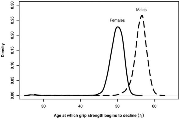
Posterior distributions of the ages (years) at which grip strength begins to decline (t₂) for females (solid line) and males (dashed line).

Secular trend in peak grip strength

Also, there is an increasing secular trend in peak grip strength, with the estimated peak for the 1980–1989 cohort extrapolated assuming that, in the future, their rate of change remains the same and that they attain their peak at t₁. The posterior probabilities of each cohort having a higher peak than its preceding cohort range from 0.83 to almost 1 and are shown in Figure 3. Note that this increasing secular trend is not attributable to concurrent secular trends in body size as this model is adjusted for body size.

Fig. 3.

Posterior mean peak grip strength vs. birth cohort, by sex. Vertical bars indicate 95% posterior credible intervals. The probabilities shown are posterior probabilities of a cohort's mean grip strength being larger than that of the preceding cohort. Peak grip strength for the 1980–1989 cohort was extrapolated assuming that, in the future, their rate of change remains the same and that they attain their peak at t₁.

Influence of risk factors on the grip strength trajectory

The last nine rows of Table 3 contain estimates for the risk factors and their interactions included in the final models, by sex and controlling for body size and secular trends. For males, higher birth weight and never smoking were associated with a higher young adulthood rate of increase in grip strength, and higher birth weight was associated with higher peak grip strength, as well. An interaction between current drinking and ever smoking was significantly associated with the later adulthood rate of decline. The order of the rates of decline for the four combinations of ever smoking and current drinking was difficult to interpret, and there are likely unmeasured confounders that are causing potentially counterintuitive results. For example, for men who currently do not drink, having ever smoked was associated with a significantly slower rate of decline in grip strength after t₂ (−0.57 + 0.42 = −0.15 kg/year). For women, current drinking was associated with higher peak grip strength, sport activity was positively associated with the young adulthood rate of increase in grip strength, and, for those who currently drink, sport activity levels were associated with higher peak grip strength.

These data arise from an observational study, and these significant associations cannot be said to be causal. However, the finding that males with lower birth weight tend to have lower adult grip strength, even after adjusting for adult body size, is supported by previous research (Inskip et al., 2007; Kuh et al., 2002; Yliharsila et al., 2007). Figure 4 illustrates the estimated mean grip strength trajectories for males with birth weights one standard deviation below the mean (2.87 kg, dashed line) and one standard deviation above the mean (4.07 kg, solid line).

Fig. 4.

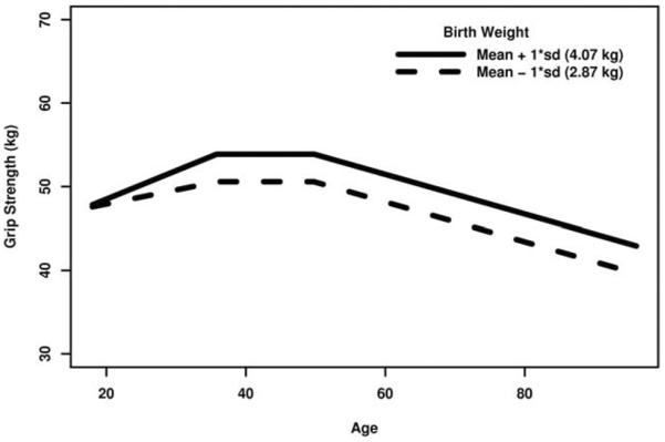
Grip strength vs. age trajectories, by birth weight (males, assuming birth cohort 1950–1959, BMI at age 45 is 25 kg/m², all other continuous covariates at their sex-specific means, and all categorical covariates at their reference levels).

Figure 5 illustrates the between-imputation variation in the posterior density for the parameters corresponding to the interactions between birth weight and the lower slope (left panel) and between birth weight and peak grip strength (right panel) as well as the computation of the posterior P-value for each. In each panel of Figure 5, the thin black lines represent single imputations, whereas the thick black line represents the t-approximation to the posterior pooled over all five imputations; the area of the shaded region (P) is equivalent to the posterior P-value. Because of the large proportion of missing birth weights (see Table 2), there is noticeable variability in the location of these posterior densities, particularly for the interaction effect between birth weight and peak grip strength. Nevertheless, this variability is small enough that significant associations between birth weight and the grip strength trajectory were still detectable.

Fig. 5.

Posterior densities for the effects of birth weight on the lower slope (left panel) and on peak grip strength (right panel), by imputation. “P” represents the posterior P-value.

DISCUSSION

We have illustrated the application of Bayesian statistical methods to handle a complex longitudinal analysis involving a model with multiple unknown change-points, time-varying covariates, unbalanced observation times, and missing response and covariate data. Unknown change-points turn a linear model into a nonlinear model. Although a nonlinear mixed model can be fit in SAS PROC NLMIXED (Littell et al., 2006) or the R function nlme (Pinheiro et al., 2009), these programs cannot directly handle the joint modeling of a time-varying covariate and response as specified here. Within the Bayesian framework, such a model is handled easily with a few more lines of code in WinBUGS (although with large datasets, this adds considerably to the computation time). The new PROC MCMC in SAS v9.2 can also handle the plateau model as specified here with independent random effects. The BMI model, however, with correlated random effects, would require additional programming in SAS as the current version of PROC MCMC does not allow multivariate distributions (Chen, 2009) as would be required for the prior distribution of the random effects covariance matrix.

Additionally, it is straightforward to combine posterior inferences over MIs to handle missing data. Although not illustrated to its full potential here, posterior inferences are extremely powerful in their ability to handle nonlinear functions of the model parameters. Although output from SAS PROC MIXED or SAS PROC NLMIXED can be sent to PROC MIANALYZE to combine inferences over MIs, this becomes more difficult for nonlinear functions of the model parameters. Bayesian posterior inference handles such a problem automatically; the posterior distribution of a nonlinear function of parameters is easily estimated as the empirical distribution of the realizations of this nonlinear function over the joint posterior sample of the model parameters.

In a longitudinal analysis of the adult dominant hand grip strength trajectory, we found that, on an average, men and women attain peak grip strength around age 36 years but women begin to decline sooner (age 50 years for women and 56 years for men). Once they begin to decline, however, men lose grip strength at a faster rate relative to their peak. Also, we found increasing secular trends in peak grip strength for both men and women that are not attributable to concurrent secular trends in body size. Regarding the evaluation of risk factors, after adjusting for body size, we found significant associations between the grip strength trajectory and birth weight (men only), smoking (men only), alcohol consumption (men and women), and sports activity (women only).

It is important to note the assumptions implicit in the model we have presented. No cohort was observed over the entire adult age range. For younger cohorts, we have no information about the rate of change in grip strength at older ages, and, for older cohorts, we have no information about the rate of change in grip strength at younger ages. This is a problem inherent to the study design. That is, for a given birth cohort, the age range over which the grip strength trajectory is unobserved corresponds to either (a) calendar years during which measuring grip strength was not yet part of the Fels Longitudinal Study protocol or (b) ages not yet attained. The analysis presented here assumes that the early adulthood and later adulthood rates of change in grip strength do not differ between birth cohorts. Secular trends (that is, differences in mean grip strength between cohorts over an age range at which they were all observed) are therefore modeled as differences in cohort-specific intercepts. In the plateau model, these intercepts correspond to the cohort-specific mean peak grip strengths. For younger cohorts, the interpretation of the intercept as the peak grip strength requires an extrapolation under the assumption that the future trajectory will have the same rate of change and will peak at the same time as older cohorts.

An additional assumption is that the beginning and ending ages of the plateau are common to all cohorts. For the present analysis, estimation of the change-point t₁ is based mostly on data from the 1950 and 1960 cohorts, and estimation of t₂ is based mostly on data from the 1930 and 1940 cohorts. As the youngest cohorts continue to age, we may find in the future that they reach their peak at a different age and/or that they begin to decline at a different age than did older cohorts.

Our method of handling missing data, MI, depends on the assumption of ignorability (Little and Rubin, 2002). In our analysis, this assumption is equivalent to the assumption that the data are “missing at random” (MAR); that is, the missing data values for a variable can be predicted based on the relationship between that variable and the remaining variables using the cases where they are jointly observed. If that relationship is different for the missing and nonmissing values, then the missing data are “not missing at random” (NMAR), and MI could potentially lead to biased parameter estimates. The MAR assumption, however, is not testable using observed data. To assess the impact of potential departures from MAR, one could use a sensitivity analysis (Carpenter et al., 2007; Daniels and Hogan, 2008). The results in the final models (Table 3) that would be most sensitive to a departure from MAR are those relating to sports activity and birth weight, as they have the largest proportions of missing values among the risk factors included in the final models.

In summary, longitudinal data analysis requires handling not only serial correlation but quite often also time-varying covariates and missing data (both for time-varying and time-invariant variables). The analysis presented here provides an example of how to handle these issues as well as the estimation of unknown change points, in the context of a Bayesian model for unbalanced longitudinal data.

LITERATURE CITED

- Baecke JA, Burema J, Frijters JE. A short questionnaire for the measurement of habitual physical activity in epidemiological studies. Am J Clin Nutr. 1982;36:936–942. doi: 10.1093/ajcn/36.5.936. [DOI] [PubMed] [Google Scholar]
- Carpenter JR, Kenward MG, White IR. Sensitivity analysis after multiple imputation under missing at random: a weighting approach. Stat Methods Med Res. 2007;16:259–275. doi: 10.1177/0962280206075303. [DOI] [PubMed] [Google Scholar]
- Chen F. Bayesian modeling using the MCMC procedure. Paper 257–2009. Proceedings of the SAS® Global Forum 2009 Conference; Cary, NC: SAS Institute, Inc; 2009. [Google Scholar]
- Chumlea WC, Choh AC, Lee M, Towne B, Sherwood RJ, Duren DL, Czerwinski SA, Siervogel RM. The first seriatim study into old age for weight, stature and BMI: the Fels longitudinal study. J Nutr Health Aging. 2009;13:3–5. doi: 10.1007/s12603-009-0001-5. [DOI] [PMC free article] [PubMed] [Google Scholar]
- Daniels MJ, Hogan JW. Missing data in longitudinal studies: strategies for Bayesian modeling and sensitivity analysis. Chapman and Hall/CRC; Boca Raton: 2008. [Google Scholar]
- de Groot JA, Janssen KJ, Zwinderman AH, Moons KG, Reitsma JB. Multiple imputation to correct for partial verification bias revisited. Stat Med. 2008;27:5880–5889. doi: 10.1002/sim.3410. [DOI] [PubMed] [Google Scholar]
- Diggle PJ, Heagerty P, Liang K-Y, Zeger SL. Analysis of longitudinal data. Oxford University Press; Oxford: 2002. [Google Scholar]
- Fitzmaurice G, Laird NM, Ware JH. Applied longitudinal analysis. Wiley; Hoboken: 2004. [Google Scholar]
- Frederiksen H, Hjelmborg J, Mortensen J, McGue M, Vaupel JW, Christensen K. Age trajectories of grip strength: cross-sectional and longitudinal data among 8,342 Danes aged 46 to 102. Ann Epidemiol. 2006;16:554–562. doi: 10.1016/j.annepidem.2005.10.006. [DOI] [PubMed] [Google Scholar]
- Fuller WA. Measurement error models. Wiley; New York: 1987. [Google Scholar]
- Gelfand AE, Smith AFM. Sampling-based approaches to calculating marginal densities. J Am Stat Assoc. 1990;85:398–409. [Google Scholar]
- Gelman A, Carlin JB, Stern HS, Rubin DB. Bayesian data analysis. Chapman and Hall/CRC; Boca Raton: 2004. [Google Scholar]
- Harrell FE., Jr . Hmisc: Harrell Miscellaneous. R package version 3.7–0. 2009. with contributions from many other users. [Google Scholar]
- Harris T. Muscle mass and strength: relation to function in population studies. J Nutr. 1997;127:1004S–1006S. doi: 10.1093/jn/127.5.1004S. [DOI] [PubMed] [Google Scholar]
- Inskip HM, Godfrey KM, Martin HJ, Simmonds SJ, Cooper C, Sayer AA. Size at birth and its relation to muscle strength in young adult women. J Intern Med. 2007;262:368–374. doi: 10.1111/j.1365-2796.2007.01812.x. [DOI] [PMC free article] [PubMed] [Google Scholar]
- Kallman DA, Plato CC, Tobin JD. The role of muscle loss in the age-related decline of grip strength: cross-sectional and longitudinal perspectives. J Gerontol. 1990;45:M82–M88. doi: 10.1093/geronj/45.3.m82. [DOI] [PubMed] [Google Scholar]
- Kuh D, Bassey J, Hardy R, Aihie Sayer A, Wadsworth M, Cooper C. Birth weight, childhood size, and muscle strength in adult life: evidence from a birth cohort study. Am J Epidemiol. 2002;156:627–633. doi: 10.1093/aje/kwf099. [DOI] [PubMed] [Google Scholar]
- Littell RC, Milliken GA, Stroup WW, Wolfinger RD, Schabenberger O. SAS for mixed models. 2nd ed SAS Publishing; Cary, NC: 2006. [Google Scholar]
- Little RJA, An H. Robust likelihood-based analysis of multivariate data with missing values. Stat Sin. 2004;14:933–952. [Google Scholar]
- Little RJA, Rubin DB. Statistical analysis with missing data. Wiley; Hoboken: 2002. [Google Scholar]
- Liu M, Taylor JM, Belin TR. Multiple imputation and posterior simulation for multivariate missing data in longitudinal studies. Biometrics. 2000;56:1157–1163. doi: 10.1111/j.0006-341x.2000.01157.x. [DOI] [PubMed] [Google Scholar]
- Lohman TG, Roche AF, Martorell R, editors. Anthropometric standardization reference manual. Human Kinetics Publishers; Champaign, IL: 1988. [Google Scholar]
- Lunn DJ, Thomas A, Best N, Spiegelhalter D. WinBUGS—a Bayesian modelling framework: concepts, structure, and extensibility. Stat Comput. 2000;10:325–337. [Google Scholar]
- Pinheiro J, Bates D, DebRoy S, Sarkar D, R Core Team . nlme: linear and nonlinear mixed effects models. R package version 3.1–96 2009. [Google Scholar]
- R Development Core Team . R: a language and environment for statistical computing. R Foundation for Statistical Computing; Vienna, Austria: 2009. [Google Scholar]
- Roche AF. Growth, maturation and body composition: the Fels longitudinal study 1929–1991. Cambridge University Press; Cambridge: 1992. [Google Scholar]
- Rolland Y, Czerwinski S, Abellan Van Kan G, Morley JE, Cesari M, Onder G, Woo J, Baumgartner R, Pillard F, Boirie Y, Chumlea WC, Vellas B. Sarcopenia: its assessment, etiology, pathogenesis, consequences and future perspectives. J Nutr Health Aging. 2008;12:433–450. doi: 10.1007/BF02982704. [DOI] [PMC free article] [PubMed] [Google Scholar]
- Rubin DB. Multiple imputation for nonresponse in surveys. Wiley; New York: 1987. [Google Scholar]
- Schafer JL. Analysis of incomplete multivariate data. Chapman & Hall/CRC; Boca Raton: 1997. [Google Scholar]
- Schafer JL, Yucel RM. Computational strategies for multivariate linear mixed-effects models with missing values. J Comput Graph Stat. 2002;11:437–457. [Google Scholar]
- Siddique J, Belin TR. Multiple imputation using an iterative hot-deck with distance-based donor selection. Stat Med. 2008;27:83–102. doi: 10.1002/sim.3001. [DOI] [PubMed] [Google Scholar]
- Sorkin JD, Muller DC, Andres R. Longitudinal change in height of men and women: implications for interpretation of the body mass index: the Baltimore longitudinal study of aging. Am J Epidemiol. 1999;150:969–977. doi: 10.1093/oxfordjournals.aje.a010106. [DOI] [PubMed] [Google Scholar]
- Sturtz S, Ligges U, Gelman A. R2WinBUGS: a package for runningWinBUGS from R. J Stat Softw. 2005;12:1–16. [Google Scholar]
- van Buuren S, Brand JPL, Groothuis-Oudshoorn CGM, Rubin DB. Fully conditional specification in multivariate imputation. J Stat Comput Simul. 2006;76:1049–1064. [Google Scholar]
- Yliharsila H, Kajantie E, Osmond C, Forsen T, Barker DJ, Eriksson JG. Birth size, adult body composition and muscle strength in later life. Int J Obes (Lond) 2007;31:1392–1399. doi: 10.1038/sj.ijo.0803612. [DOI] [PubMed] [Google Scholar]