Ethylene glycol revisited: Molecular dynamics simulations and visualization of the liquid and its hydrogen-bond network

Abstract

Molecular dynamics simulations of liquid ethylene glycol described by the OPLS-AA force field were performed to gain insight into its hydrogen-bond structure. We use the population correlation function as a statistical measure for the hydrogen-bond lifetime. In an attempt to understand the complicated hydrogen-bonding, we developed new molecular visualization tools within the Vish Visualization shell and used it to visualize the life of each individual hydrogen-bond. With this tool hydrogen-bond formation and breaking as well as clustering and chain formation in hydrogen-bonded liquids can be observed directly. Liquid ethylene glycol at room temperature does not show significant clustering or chain building. The hydrogen-bonds break often due to the rotational and vibrational motions of the molecules leading to an H-bond half-life time of approximately 1.5 ps. However, most of the H-bonds are reformed again so that after 50 ps only 40% of these H-bonds are irreversibly broken due to diffusional motion. This hydrogen-bond half-life time due to diffusional motion is 80.3 ps. The work was preceded by a careful check of various OPLS-based force fields used in the literature. It was found that they lead to quite different angular and H-bond distributions.

Graphical abstract

Highlights

• •We simulated liquid ethylene glycol classically.
• •Four OPLS-AA based force fields were compared.
• •Hydrogen bonds were identified by geometrical criteria.
• •Lifetimes of hydrogen bonds were obtained using the population correlation formalism.
• •A visualization of individual hydrogen-bond lifetimes was implemented and clustering of hydrogen bonds was observed.

1. Introduction

Liquid ethylene-glycol (EG) has many applications. It is probably best known as anti-freeze protection in cooling/heating systems as well as in de-icing solutions for vehicles and runways of airports. Amongst other uses it serves as ingredient of electrolytic capacitors, printer's inks and it is used as a solvent. It is raw material for the production of explosives and synthetic waxes. EG is a sweetly tasting odorless liquid and it is toxic if swallowed in large amounts [1], [2]. EG and EG–water mixtures have another important application field. Such solvents are used as a media with variable viscosity in experimental studies of the solvent dynamics effect on electrochemical reactions (see, for example [3], [4]). In the framework of modern quantum mechanical theory of electron transfer some quantities which affect reaction kinetics (effective frequency factor, solvent reorganization energy) can be calculated by using the complex dielectric spectrum of a polar medium measured experimentally. Understanding the nature of characteristic solvent modes and their relaxation times forming the dielectric response is an important problem. The behavior of some solvent modes which may serve as electron transfer coordinates depends, in turn, on the interplay between the EG–EG and EG–H₂O inter-molecular H-bonds, as well as on H-bonds in an EG molecule. Indeed, properties of liquid ethylene-glycol can be backtracked to its structure as a flexible molecule with hydroxyl groups that can participate in hydrogen bonding (Fig. 1). A deeper insight into the microscopic nature of H-bonding in this solvent can be gained from molecular dynamics simulations.

Fig. 1.

Two hydrogen-bonded EG molecules.

First simulation studies of the hydrogen-bonds in liquid EG via molecular dynamics (MD) simulations were performed by Padró et al. [5] in the scope of a comparison of the hydrogen-bond structure and hydrogen-bond lifetime of various alcohols. Methanol and ethanol are reported to build chainlike structures [6], [7], whereas ethylene glycol and glycerol show three-dimensional patterns. The effects of different force fields on the dihedral angle distributions, the radial distribution functions (RDFs), the mean number of hydrogen-bonds per molecule, and the dispersion coefficients were tested on liquid EG in [8]. Some of these quantities will also be analyzed in the present work. Percentages of hydrogen-bonded molecules in a mixture of liquid EG and water were presented for various concentrations and temperatures in [9]. Dihedral probability distributions for the OCCO and HOCC angles were calculated for OPLS like force fields in [10]. A further interesting feature of EG is its ability to build intra-molecular hydrogen-bonds. Their existence was suggested and backed up by various experimental works [11], [12], [13].

The analysis of hydrogen-bonding requires more than simple statistical criteria such as the average number of hydrogen-bonds per molecule: One hydrogen-bond between two molecules can be characterized by its energy and a few (usually 3) geometrical parameters. Chains of hydrogen-bonds need parameters describing their length and bifurcation. All these parameters are associated with specific lifetimes and other dynamical parameters. With that in mind, we believe that a direct and interactive visualization of the hydrogen-bond network and its individual lifetime would be beneficial but has, as far as we know, not yet been attempted. As a first step towards this aim a new molecular visualization tool was implemented as an extension to the Vish Visualization shell [14].

In the present work liquid ethylene-glycol at room temperature and its hydrogen-bonds are reinvestigated thoroughly. The methods Section 2 describe the details of the MD simulation and the methods for data reduction and visualization. All results are discussed in Section 3. Structural results such as the radial distribution functions, the dihedral angle distributions, the mean number of hydrogen-bonds per molecule, and the percentage of molecules with exactly n hydrogen-bonds are given in Section 3.1. In Section 3.2 the dynamical results are summarized together with the visualization of the hydrogen-bond lifetimes.

2. Models and methods

2.1. MD simulations

MD simulations were performed using the DL_POLY_4 package [15]. The density of EG was set to 1.1003 g/cm³, corresponding to the experimental value. The number of conformation states, 27, was identified in [16], based on the three main torsional degrees of freedom of EG: the backbone dihedral angle OCCO and the two HOCC angles. Due to symmetry the number of distinguishable conformers is reduced to ten. These conformation states were studied by Hartree–Fock calculations with the 4-31G basis set already in 1972 [16]. The search for the most stable conformers continued as better methods became available, i.e., [17] on the MP2/6–311G(3df, 3dp) level or [18] using HF/6–31++G** and MP2. In both works, it was shown that the tGg′ (the notation was introduced in [16]) isolated monomer is the most stable one, a prediction that has also been backed up by results from electron diffraction [19] and infrared spectroscopy [11], [20].

Over time, various all-atom OPLS force fields were used to describe the inter- and intra-molecular interactions of EG. The basic model parameters were taken from Jorgensen's paper for carbohydrates (OPLS-AA) [21]. A first modification of this field involved scaling the electrostatic interactions (OPLS-AA-SEI) [22]; a second modification in order to improve the density and heat of vaporization called OPLS-AA-SEI-M was presented in [10]. A specially tailored force field for ethylene glycol for the gromacs software was published in [23] (hereafter referenced by ‘Cordeiro’). We converted all these force fields into the format used in DL_POLY_4 enabling comparison to each other. Their various parameters are summarized in Table 1, Table 2, Table 3, Table 4.

Table 1.

Lennard–Jones parameters and partial charges for EG. Footnotes a, b, c, and d see Table 4.

Atom	Amber type	σ (°)	ε (kcal/mol)	q (in a.u.)
H on C	HC	2.50	0.030	0.06
C	CT	3.50	0.066	0.145abc, 0.165d
O in Diol	OH	3.07abcd, 3.0e	0.170	− 0.700abc, − 0.720d
H in OH	HO	0.00	0.00	0.435

Table 2.

Bond stretching parameters for EG.

Atom	Kr (kcal/mol Å)	req (Å)
CT–OH	320.0	1.410
CT–CT	268.0	1.529
CT–HC	340.0	1.090
OH–HO	553.0	0.945

Table 3.

Angle bending parameters for EG.

Amber types	θeq (°)	Kθ (kcal/(mol rad2))
CT–CT–HC	110.7	37.5
CT–CT–OH	109.5	50.0
CT–OH–HO	108.5	55.0
HC–CT–HC	107.8	33.0
HC–CT–OH	109.5	35.0

Table 4.

Torsional parameters (kcal/mol) for EG.

Type	V1	V2	V3
HC–C–C–HC	0.0	0.0	0.318abc, 0.0d
HC–C–OH–HC	0.0	0.0	0.45abc, 0.0d
C–C–OH–HO	2.674a, − 0.004bc, 0.396d	− 2.883a, − 0.629bc, − 0.750d	1.026a, 0.035bc, 1.03d
OH–CT–CT–HC	0.0	0.0	0.468abc, 0.0d
HC–C–OH–HO	0.0	0.0	0.45abc, 0.0d
OH–C–C–OH	9.066a, 4.78bc, 2.993d	0.0a, − 3.593bc, − 0.654d	0.0a, − 0.887bc, 2.820d

^aOPLS-AA, Table 5 in [21] for carbohydrates, scaling of 1–4 vdW and Coulomb interactions with 0.5.

^bOPLS-AA-SEI [22]: scaling 1–4 interactions with 0.5, 1–5 interactions with 0.8.

^cOPLS-AA-SEI-M [10]: scaling 1–4 vdW with 0.65 and 1–4 Coulomb with 0.6, 1–5 interactions with 0.8.

^dOPLS-AA from Cordeiro et al. [23]: scaling 1–4 with 0.5, no 1–5 scaling.

For force fields of the OPLS-AA type the bond and valence-angle potentials are harmonic

$$E_{\mathit{bond}}={\Sigma }_{\mathit{bonds}}{\mathit{K}}_r{\left(r-r_{\mathit{eq}}\right)}^2\text{,}$$

$$E_{\mathit{angle}}={\Sigma }_{\mathit{angles}}{K}_{\theta }{\left(\theta -{\theta }_{\mathit{eq}}\right)}^2\text{,}$$

whereas torsional motion is represented by a Fourier series with coefficients V₁, V₂, and V₃,

$$E_{\mathit{torsion}}={\Sigma }_i\frac{V_1^i}{2}\left(1+cos\left({\varphi }_i\right)\right)+\frac{V_2^i}{2}\left(1-cos\left(2{\varphi }_i\right)\right)+\frac{V_3^i}{3}\left(1+cos\left(3{\varphi }_i\right)\right)\text{,}$$

with the dihedral angle φ_i. Scaling factors for 1–4 and 1–5 electrostatic and van der Waals interactions were used appropriately for the four different force fields (see footnotes a, b, c, and d in Table 4). The combination rules for the OPLS force fields were used to define the van der Waals parameters:

$${\sigma }_{\mathrm{ij}}=\sqrt{{\sigma }_{\mathrm{ii}}{\sigma }_{\mathrm{jj}}},{\mathrm{ϵ}}_{\mathrm{ij}}=\sqrt{{\mathrm{ϵ}}_{\mathrm{ii}}{\mathrm{ϵ}}_{\mathrm{jj}}}\text{.}$$

For the initial structure of the EG molecules in the simulation cell the tGg′ geometry, the most stable conformer in the gas state, was chosen. After obtaining an equilibrated system in the NVE ensemble from the original OPLS-AA force field we started each MD simulation run with a 10 ps equilibration period at 1000 K in the NVT ensemble with a Nosé–Hoover thermostat and a time step of 0.5 fs, followed by 10 ps at 250 K. This was followed by a further equilibration for 100 ps at the final temperature (298 K) with a 1 fs time step and a final equilibration in the NPT ensemble with a Berendsen [24] thermostat (1 ps relaxation time) and barostat (3 ps relaxation time) for another 100 ps. The system contained 512 EG molecules in a cubic box with periodic boundary conditions. Ewald summation handled long range electrostatic forces. Short-range forces were cut off at 10 Å. Two history files were created: One with a stride of 50 fs and a total simulation time of 1 ns, and one with a stride of 5 fs and a total simulation time of 100 ps. We carefully checked our simulation for convergence of the structural properties and their statistical significance by inspecting block averages.

2.2. Hydrogen-bond structure and lifetime

The hydrogen-bond connectivity information was obtained for each time step by using the common criterion R_OO < R_OOc AND R_OH < R_OHc AND ϕ < ϕ_c [5], [8], [9], [25], [26], where R_OH is the distance between acceptor oxygen and donor hydrogen and R_OO is the distance between acceptor oxygen and donor oxygen as displayed in Fig. 2. The criterion states that both of these distances must simultaneously be smaller than the critical distances R_OHc and R_OOc respectively; these critical distances are the positions of the first minima of the corresponding RDFs. ϕ_c is the valence angle between donor hydrogen, donor oxygen and acceptor oxygen (H—O…O); the chosen critical angle is ϕ_c = π/6 for inter-molecular hydrogen-bonds and ϕ_c = π/3 for intra-molecular hydrogen-bonds [10], [27], [28]. The connectivity information is the basis for the lifetime calculation. For each time step and each entry in the connectivity matrix, which is for each hydrogen-bond, the same entry is searched for in the following time steps. The process is visualized in Fig. 3 for an example trajectory with three time steps and a stride of 0.2 ps: Each atom is given a unique index. The columns Oa, Od and Hd are the indices of the oxygen acceptor (Oa), oxygen donor (Od) and hydrogen donor (Hd) atoms that participate in hydrogen-bonding. The lifetime of each hydrogen-bond at each time step is stored in the column life. It represents the number of time steps a hydrogen-bond still lives within the simulation. This individual lifetime is visualized in Section 3.2.

Fig. 2.

Definition of the lengths R_OO and R_OH and the angle ϕ as used in the criterion for hydrogen-bonding.

Fig. 3.

Example of connectivity and lifetime information for hydrogen-bonds for three time steps. The columns Oa, Od and Hd contain the unique atom indices of acceptor and donor atoms participating in the hydrogen-bond. The lifetime of each hydrogen-bond is given in an extra column “life”.

A statistical quantity for the average hydrogen-bond lifetime is not easily defined, but can be obtained using the population correlation formalism of Chandra [27], which is similar to the correlation function used in [25] based on [29]. The time correlation function

$$S_{\mathit{HB}}\left(\mathrm{t}-{\mathrm{t}}_0\right)=<\mathrm{h}\left({\mathrm{t}}_0\right)\mathrm{H}\left(\mathrm{t}\right)>/<\mathrm{h}>$$ (1)

measures the continuous presence of a hydrogen-bond from the initial time t₀ up to time t. The mean value over all hydrogen-bonds is indicated by <…>. Picking out a certain hydrogen-bond, the function h(t₀) = 1, if the hydrogen-bond exists at time t₀, otherwise h(t₀) = 0. This is equivalent with the appearance of this particular hydrogen-bond in the connectivity information at time t₀. The function H(t) = 1, if the specified hydrogen-bond for which h(t₀) = 1 survives up to time t, otherwise H(t) = 0. This is equivalent with the continuous appearance of this hydrogen-bond in the connectivity matrix from time t₀ up to t. Therefore this function can easily be calculated using the individual lifetime information stored in column “life” in Fig. 3. One just has to count the number of individual lifetimes that are smaller than t–t₀ and average over all initial values t₀. It is useful to include only the first half of the simulation, because the lifetimes decrease towards the end due to the finite simulation time; all lifetimes in the last time step are equal to 1. Since we deal with discrete time steps the function S_HB(t) natively also depends on the size of the time step or stride t*, because within t*, the hydrogen-bond can break and reform without being counted as broken.

2.3. Visualization methods

The large amount of data produced by the numerical simulation requires appropriate visualization methods that allow quick exploration and analysis. Existing visualization packages (Chavent et al. [30] presented an overview of recent methods and software) already provide multifarious functionalities, but in order to be able to have full control over the data analysis and visualization process we chose to employ a visualization framework that allows easy modification and adaption from the basic level. The Vish Visualization shell is a modular C++ framework for scientific visualization providing both high-level functionality, such as a GUI, scripting and data I/O for complex data types, as well as hardware-oriented implementations such that we can utilize features of modern graphics cards (GPUs) for displaying the molecular data. While a conventional rendering approach for molecules would use the data sets to create some geometry (usually in the form of triangles), we intend to avoid creating any geometry and just load the molecular data “as is” into the graphic card's memory. It is then up to the graphics card and specific GPU code (shaders) to produce a meaningful graphical representation from these data. The CPU work is limited to mere data management interactions, but not burdened with any computational efforts, thereby achieving maximal performance with interactively adjustable visualization of large molecular data.

Vish uses a data layout based on the mathematics of fiber bundles, differential geometry and geometric algebra [31] called the F5 data model. This data model allows developing systematic and highly reusable data processing and visualization modules independent from a specific application domain. Extending this model to molecular data is straightforward. The data structures are efficiently representable in the HDF5 [32] file format, which was originally developed by the National Center for Supercomputing Applications (NCSA) for use in the high performance computing community. A lightweight C library, the “F5” library, provides a set of high-level functions for easy I/O of complex datasets into this HDF5 based layout [33].

The F5 data model is based on the theory of fiber bundles. Here, any data is modeled by a total space being constructed from a base space representing the geometry and a fiber space representing the data attached to the geometry. The data-fields used to visualize molecules and hydrogen-bonds are summarized in Table 5. The base space is represented by the atom's coordinates (vertices) and the bonds (edges). The fiber space for the vertices consists of the atom types and masses, for the edges of the edge types and bond-lifetimes. The lifetime of chemical bonds was set to zero. This data is embedded in geometrical grid objects and given for each time step called, time-slice in the f5 data model. Time independent data such as the type and mass field is stored only in the first time-slice and provided by links in all other time steps. This functionality is both possible in memory (reference-counting) as well as in an HDF5 file (symbolic links to datasets) and allows saving disk/memory space without need to modify the access procedure on the data structure: A field can still be requested at any time step, though it might actually be retrieved from the first time step. A stand-alone command line based converter was developed in the C programming language. We utilize the open matio library [34] for data conversion since that allows reading Matlab's .mat files of all supported versions. The converter takes a .mat file with the whole history data stored in a structure as an argument and creates the F5 file.

Table 5.

Data-fields used for molecular visualization.

Data-field	Description	Data type	Time dependent
Vertices	Atom coordinates	Float × 3	Yes
Type	Type of the atoms	Unsigned short × 1	No
Mass	Atom mass	Float × 1	Optional
Edges	Connectivity of hydrogen and chemical bonds	Unsigned long × 2	Yes (partially)
Edge type	Type of bond: 0 for hydrogen-bond, 1 for single bond and 2 for double bond	Unsigned short × 1	Yes (partially)
Lifetime	Lifetime of a bond in steps: 0 for chemical bonds	Float × 1	Yes

We implemented two modules for the direct visualization of the molecular data, one for displaying the atoms and one for displaying the bonds. Atoms are displayed as small spheres. Spheres can be computed via ray tracing [35], by finding intersection points between light rays solving the sphere equation, or by tessellating the sphere into triangles and use of a projective rendering technique. As we aim to display many atoms very efficiently both techniques have disadvantages in the OpenGL rendering based framework. OpenGL itself is a projective based renderer, highly optimized for handling triangular surface data. Still, for achieving a good visual approximation of a sphere many triangles would be required. Ray tracing is not supported by OpenGL. Thus, we apply a hybrid technique. We draw so called impostor objects that look like a sphere, but are small rectangles carrying an image (texture) of a sphere, which is computed via ray tracing in a fragment shader. Fig. 4 illustrates the technique. From the eye of the beholder no difference to a real 3D sphere is visible.

Fig. 4.

Impostor objects are small camera oriented rectangles carrying an image (texture) of a sphere computed by ray tracing. The texture is computed in real time on the GPU in a fragment shader.

To create the camera oriented rectangles we use point primitives, the fastest geometrical primitives for rendering. This comes with a limitation of a maximum size dependent on the used graphics hardware. Moreover, its size has to be specified in pixels on the screen and not as a size in 3D space. The pixel size has to be computed explicitly from model view space to screen pixel space that usually is done by the OpenGL pipeline itself. Two points with a distance of a specified size are placed in model view space and transformed to clip coordinates via normalized device coordinates to window coordinates, where the distance can be measured in pixels. Fig. 5 illustrates different steps of the implementation showing the scaled point, their shape and depth computed by the sphere equation and the final shaded impostors. A Vish rendering module allows for adjusting the size of the spheres and controlling the colors by a scalar field, a scalar range and a color map. The impostor technique allows rendering of one million atoms at a frame rate of 20 frames per second on the screen, measured on an Intel Xeon i7 X5650@2.67 Ghz equipped with a NVIDIA Quadro 5000 graphics card (GPU).

Fig. 5.

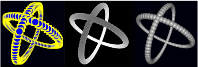
Different development stages of the impostors illustrating the technique. From left to right: Perspective scaled points colored by solving the sphere equation in a fragment shader, depth value computed from the sphere equation, and final combination of normal vector and depth via Blinn shading.

Chemical bonds are visualized by cylindrical objects. Three types of bonds are illustrated by different geometries: cylinders, striped cylinders and spirals. These are approximated by triangular surfaces. To avoid creating large amount of triangular data in the main memory (RAM) we utilize a geometry shader that allows to load lines on the GPU and create triangles there, thus avoiding slow data transfer from RAM to GPU. The developed Vish rendering module provides parameters controlling the width of the bonds, the number of stripes, and a parameter to remove long bonds that might arise due to periodic boundary conditions. Two scalar fields control the color and geometric type of the bonds.

3. Results and discussion

3.1. Liquid structure

In order to understand the hydrogen-bond structure, characteristic geometrical features of liquid EG must be derived from the trajectories. The O—O and O—H(O) radial distribution functions are shown in Fig. 6. Positions of the first minima of radial distribution functions are often used to define hydrogen-bond criteria; for OPLS-AA the O—O RDF minimizes at 3.15 Å, the O—H(O) RDF at 2.35 Å. Peak positions are 2.6 Å with a height of 3.25 for O—O and 1.6 Å with a height of 3.34 for O—H(O). The only difference of the SEI improvement is larger peaks. These RDFs are typical of well-structured liquids and similar to the one obtained with other force fields [5], [8], [10], [23], [36].

Fig. 6.

O—O and O—H(O) radial distribution functions of liquid EG for OPLS-AA (solid/dashed lines) and OPL-AA-SEI-M (empty squares).

The distributions of the two HOCC angles and the middle OCCO angle are of particular interest since together they characterize nearly completely the intra-molecular geometry of the EG molecules in the liquid. These distributions were investigated also in [10], [37] for pure EG and EG/water mixtures. Fig. 7 shows the probability distributions of the HOCC angle (left) and of the OCCO angle (right) for four force fields. Interestingly, we could not reproduce the OCCO distribution of the original OPLS-AA force field as given in [10], instead the trans conformer (OCCO > 100°) is more favorable than the gauche conformer. This is also contra-intuitive to experimental findings of Buckley [20]. Experimental values for the OCCO angle are 74° [19] and 72° [38]. The results for OPLS-AA-SEI and OPLS-AA-SEI-M fit much better into the picture drawn in Ref. [10] with slight discrepancies in the positions of the maxima. For OPLS-AA-SEI-M the OCCO maximum lies at 85.5°, where Oliveira et al. reported 71.2°. The distribution of the OPLS-AA based force field of Cordeiro does not give reasonable angular distributions although we have taken great care in importing their parameters from gromacs. Due to these findings we will restrict the discussion in the remaining paper to the original field OPLS-AA and to the furthest developed field OPLS-AA-SEI-M.

Fig. 7.

Probability distribution of the HOCC and OCCO angles. For the original OPLS-AA force field [21] the HOCC maxima are at 78.3° and 180° and for the OCCO angle at 54.7° and 180°. For OPLS-AA-SEI-M [10] the first OCCO maximum is at 85.5°, the first HOCC maximum at 70.5°. Distributions for the OPLS-AA-SEI [22] and the OPLS-AA based force field of Cordeiro [23] are shown for comparison as well.

The two HOCC angles are not independent from each other, as can be seen in Fig. 8 for OPLS-AA (left) and OPLS-AA-SEI-M (right). To begin with OPLS-AA, we observe that if the first HOCC angle is positive, the probability of the second angle being negative is higher than the one of the second being positive. For the favored trans configuration for OCCO this means that most of the molecules are in gTg′ configuration. This is exactly not the case for OPLS-AA-SEI-M, where the gauche orientation for OCCO (|OCCO| < 130°) dominates and a majority of molecules is found in the gGg configuration. A lower probability is found for gXg (OPLS-AA) or gXg′ (OPLS-AA-SEI-M), with X either gauche (G) or trans (T), corresponding to the yellow/green peaks at 90°/90° or 70.5°/− 70.5° and vice versa. A considerable number of EG molecules also reside in the tXg⁽′⁾ conformation. For OPLS-AA-SEI-M a few reside in tXg configurations.

Fig. 8.

Two-dimensional probability distribution of the first and second HOCC angles for OPLS-AA (left) and OPLS-AA-SEI-M (right).

Fig. 9 shows a 2D probability distribution of the HOCC and OCCO angles for OPLS-AA (left) and OPLS-AA-SEI-M (right). The large difference in these pictures can be traced back to the completely different OCCO probability distributions in Fig. 7. The distribution is rather regular for OPLS-AA except for two light blue tails reaching towards the origin that will be attributed to intra-molecular hydrogen-bonding. For OPLS-AA-SEI-M the absence of a large peak at HOCC₁ = − 70.5° and OCCO = + 85.5° (g′Gg′) comes from the repulsion of the two hydrogen atoms of the hydroxyl groups that would be very close to each other in this configuration. The energetically not favorable tTt configuration is almost not visible in the corners of Fig. 9 right but is weakly present in the left part of Fig. 9.

Fig. 9.

Two dimensional probability distribution of HOCC and OCCO angles for OPLS-AA (left) and OPLS-AA-SEI-M (right).

Intra-molecular hydrogen-bonding occurs mainly for the tGg′ and gGg′ conformers with OCCO < 130° when at least one of the HOCC angles is smaller than approx. 80°. These are also the dominant contributions to the 2D angle distributions for intra-molecular H-bonded molecules, Fig. 10. In our criterion for intra-molecular hydrogen-bonds we required that the valence angle (H—O…O) should be smaller than 60°. Obviously this criterion allows for plenty (15%) of intra-molecular hydrogen-bonding in the original OPLS-AA force field (top panel) but for OPLS-AA-SEI-M only very view molecules (0.1%) fulfill it.

Fig. 10.

2D probability distributions for HOCC1/HOCC2 angles (left) and HOCC1/OCCO angles (right) for OPLS-AA (top) and OPLS-AA-SEI-M (bottom) force fields for intra-molecular hydrogen-bonded molecules.

Basic statistical values about the hydrogen-bonds are summarized in Table 6. The average number of hydrogen-bonds n_HB is 3.6 and 3.87 for OPLS-AA and OPLS-AA-SEI-M respectively. The percentage of molecules with exactly i bonds f_i has a maximum at 4 bonds per molecule (59 or 70%). Those findings are in good agreement with the work of Pardó et al. [5], who predicted n_HB = 3.9 and f₄ = 55.5%. Overall we observed large discrepancies in the dihedral angle distributions and the intra-molecular hydrogen-bonds between the two investigated force fields. This indicates that these force fields are still not quantitatively reliable for a detailed structural analysis but overall trends are described well (e.g. rdf-functions).

Table 6.

Average number of inter-molecular hydrogen-bonds n_HB, intra-molecular hydrogen-bonds n_intra per molecule and percentage of molecules with exactly i hydrogen-bonds f_i.

Force field	nHB	nintra	f0	f1	f2	f3	f4	f5	f6	f7
OPLS-AA	3.6	0.15	0.013	0.74	9.68	24.29	59.04	6.11	0.12	0.00
OPLS-AA-SEI-M	3.87	0.001	0.0015	0.09	1.96	18.77	69.6	9.43	0.16	0.00

3.1.1. Clustering

Sillrén et al. published “a statistical model of hydrogen-bond networks in liquid alcohols” [39]. This model is based on two parameters p_A and p_B. p_A is the probability of an oxygen O to act as acceptor for at least one hydrogen of another hydroxyl group and pB is the probability of O for accepting a second hydrogen, given a first H-bond already exists. These two parameters are easily evaluated from the hydrogen-bond connectivity information of both inter and intra-molecular hydrogen-bonds. Within this treatment the two OH groups of one EG molecule are considered independent from each other. For the OPLS-AA-SEI simulation p_A = 0.906 and p_B = 0.068. From these two values a variety of properties can be calculated using the formulas of [39]. The mean cluster size is  n = 30.7, suggesting a size of 15 EG molecules per cluster. The percolation limit of infinite cluster size would be reached for p_A + p_A * p_B = 1 due to Eq. (14) of Ref. [39]. For our system p_A + p_A * p_B = 0.967 is already close to this limit; 3% more hydrogen bonds per hydroxyl group (p_A = 0.936) would suffice. The fraction of OH groups that either act as roots (β) for clusters (OH's with exactly one hydrogen-bonded acceptor oxygen and a free hydrogen) or are completely unbounded w.r.t. hydrogen-bonds is called n_αβ and amounts to 3.2% in our simulation. The fraction of leaves (OH oxygen atoms that lead to branching of chains) is n_leaves = 0.094, i.e., 9.4% of all OH groups are branching points. Finally, the fraction of chain-ends is n_γ = 0.091. These values suggest large clusters built from repeatedly branched chains of hydroxyl groups in EG. This might be true for a single time step, but as can be seen from the visualization of the hydrogen-bond lifetime below, those clusters do not survive over time. Instead the hydrogen-bond network changes within timescales of picoseconds.

3.2. Dynamical quantities

3.2.1. Lifetime of hydrogen-bonds

The population correlation function S_HB(t,t*) as defined in Eq. (1) was evaluated for four different time step sizes t* and is shown in Fig. 11 for the OPLS-AA-SEI-M field. The population correlation function is surprisingly very similar for the OPLS-AA and the OPLS-AA-SEI-M force field; the differences remain within the standard deviation of the curves. Small t* includes all possible mechanisms of hydrogen-bond breaking and reforming, including fast rotational and vibrational motions. Large t* shows which hydrogen-bonds turn up repeatedly and which ones are destroyed for the rest of the simulation due to diffusional motion. The large difference in the curves for t* = 5 ps and t* = 0.005 ps can be explained in a way that almost all hydrogen-bonds are destroyed and rebuilt repeatedly due to fast molecular motions and very few of them are completely destroyed due to diffusion processes. For example after a time of 50 ps over 60% of all hydrogen-bonds that have been present at an initial time t = 0 still live (t* = 5 ps curve) but almost all of them have been broken at least once in this time interval (t* = 0.005 ps curve). The half-life defined by S_HB(t,t* = 0.005 ps) = 1 / 2 is 1.5 ps. The function could not be fitted to a single exponential function of the characteristic time and therefore we approximately equate the half-life with the life-time. The half-life of diffusional motion S_HB(t,t* = 5 ps) is 80.3 ps. The standard deviation of the population correlation functions is shown for t* = 0.5 ps as the light green background in Fig. 11 and lies in the same range for the other curves. Similar curves can be found in [5] over a much smaller time interval.

Fig. 11.

Population correlation function S_HB(t,t*) of hydrogen-bonds, where t* is the stride and therefore also the maximal time a bond can be broken without counting as broken.

Another approach to define lifetimes is by fitting two exponentials $\mathit{A}{\mathit{e}}^{-\mathit{t}/{\mathit{\tau }}_1}+\left(1-\mathit{A}\right){\mathit{e}}^{-\mathit{t}/{\mathit{\tau }}_2}$ with different characteristic life-times to the population correlation functions. The parameters and the route mean square (rms) deviation of the fit are listed in Table 7. All four functions for different t* could be fitted well with this approach, which could imply that the lifetimes are indeed dominated by a fast and a slower process. The slow process is approximately 5–6 times slower than the fast one for all t*. Speculatively, τ₁ could be associated with the life-time of diffusive translational and τ₂ with diffusive rotational motion for large t*. For small t* τ₁ might be associated with inter-molecular vibrations and τ₂ with fast molecular librations. Our results support the notion that a single number as “the” average hydrogen-bond lifetime is not very meaningful, due to the variety of effects that do play a role and separately lead to completely different lifetimes for various situations, as can be seen in Table 7 and Fig. 11.

Table 7.

Fit of the population correlation function S_HB(t,t*) with two different exponentials $\mathit{A}{\mathit{e}}^{-\mathit{t}/{\mathit{\tau }}_1}+\left(1-\mathit{A}\right){\mathit{e}}^{-\mathit{t}/{\mathit{\tau }}_2}$ and the corresponding root mean square (rms) deviation.

t* (ps)	τ1 (ps)	τ2 (ps)	A	rms deviation
0.005	4.4367	0.8667	0.5917	0.0037
0.05	10.920	2.0084	0.5341	0.0059
0.5	53.147	9.1334	0.5659	0.0046
5	213.61	32.013	0.6803	0.0055

A mechanism that differs from the simple diffusive concept followed so far was introduced for water in [40], where hydrogen-bond switching events were recorded and analyzed. A hydrogen donor changes its acceptor rapidly by rotation (jump-like within 250 fs) initiated by a change in the coordination number of the second hydration shell around the rotating H₂O. An investigation of the acceptor-donor O—O distance around hydrogen-bond breakages shows that most of the H-bonds in EG are reestablished and only few dissociate completely (494 out of an ensemble of 72,725 recorded breakages). The dissociation is indeed accompanied by a jump in the O—O distance within 200–400 fs very similar to the water picture. In [40] the OH reorientation correlation could be interpreted by combining a characteristic jump-time, which is related to the H-bond lifetime of dissociative jumps (i.e. large t*), with the O—O reorientation correlation time. Due to the internal flexibility and chain-like structure, the application of such an extended jump model was not further pursued but would be an interesting subject for future considerations.

3.2.2. Visualization of the hydrogen-bonds and their dynamics

The developed visualization modules unfold its power in the interactive exploration of the hydrogen-bond network. Hydrogen-bonded molecules can be traced until the hydrogen-bond breaks or is reformed. The visualization depends on the chosen value for t* that is the time interval of the search algorithm and physically means that hydrogen-bonds can be broken and reform within t* without recognizing them as broken. The smallest possible t* is equal to the integration time step or the dumping stride for the history file. For small t* the breaking and reforming of hydrogen-bonds due to rotations and vibrations are resolved. For large t* only the breaking due to diffusional motion is accounted for, therefore giving larger average lifetimes. Fig. 12 is a snapshot of the long run simulation, 1 ns, with the OPLS-AA-SEI-M force field and large t* = 5 ps. The maximum of the color code was chosen slightly larger than the diffusional half-life (80.3 ps) of the hydrogen-bonds. All H-bonds with lifetimes greater than 100 ps are shown in light blue. At a first glance it seems that the lifetimes are quite randomly distributed over the whole simulation box. However, small long-lived (> 100 ps) clusters of 5–20 atoms are emphasized with white circles in Fig. 12. By inspecting the same simulation with a color map up to 1 ns one cannot find any long lived clusters and the hydrogen-bonds with lifetimes > 500 ps are arbitrarily distributed over the simulation cell. This confirms our statistical results about the diffusional half-life times.

Fig. 12.

Visualization of the simulation box with chemical bonds as gray cylinders and hydrogen-bonds as dashed cylinders with color-coded lifetime.

A zoom into Fig. 12 is given in the upper panel of Fig. 13. Atoms are shown as spheres with different colors for different atom-types. This enhances the perception of single molecules. The three dimensional H-bond structure and multiple hydrogen-bonds per molecule can be observed. In the lower panel of Fig. 13 we show the short-run simulation (100 ps) with t* = 0.005 ps and an adjusted color-map. The picture of regular breaking and reforming due to rovibrational motion is confirmed. An accumulation of very long-lived clusters is also not found.

Fig. 13.

Zoom into the hydrogen-bonded three dimensional structure for the long simulation run (total 1 ns, t* = 5 ps, Δt = 0.05 ps, upper panel) and the short run (total 100 ps, t* = 0.005 ps, Δt = t*, lower panel) including spheres for atoms. The maxima of the color-maps were chosen close to the half-life time of the hydrogen-bonds.

4. Conclusion

Liquid ethylene glycol was modeled by means of classical molecular dynamics simulations with four different OPLS-based force fields. The radial distribution functions from all force fields are similar but the distributions of the intra-molecular HOCC and OCCO angles show large discrepancies. The original OPLS-AA force field favors the trans conformer, the OPLS-AA-SEI and OPLS-AA-SEI-M force fields favor the gauche conformer in accordance with experiment and ab initio calculations [11], [17], [18], [19], [20]. The mean number of inter-molecular hydrogen-bonds per EG molecule is 3.7 ± 0.2, varying only slightly with the force field. Intra-molecular hydrogen-bonds are strongly suppressed in the OPLS-AA-SEI-M case to 0.1% of the molecules compared to 15% in the original OPLS-AA field. Due to the number of possible hydrogen-bonds per molecule EG builds up three dimensional hydrogen-bonded structures with an estimated mean size of 15 molecules per cluster. A direct visualization of the hydrogen-bonded network in recently implemented visualization tools within the Vish Visualization shell gives insight into the hydrogen-bonded network and its lifetimes. It shows that there is no obvious clustering of very long-lived (> 500 ps) hydrogen-bonded clusters within the simulation cell. The lifetimes are rather randomly distributed over the whole cell. Hydrogen-bonds break regularly in timescales of a few picoseconds due to rovibrational motions and might be reformed later on. Clusters of 5–20 relatively long-lived hydrogen-bonds (> 100 ps) can be observed. The irreversible destruction of hydrogen-bonds due to diffusion happens on a time-scale of 80 ps. These results are again relatively independent of the force field. This work is considered as a first step towards interpreting experimentally measured dielectric properties of EG (in the near future also of EG/water mixtures) in terms of lifetimes of hydrogen-bonds, rovibrational motions, and conformer changes.

References

- 1.E.S.B. Merck, C. Inc. An Encyclopedia of Chemicals, Drugs, and Biologicals. 1989. (Rahway, NJ) [Google Scholar]
- 2.Agency for toxic substances, disease registry (ATSDR) U.S. Department of Public Health and Human Services, Public Health Service; Atlanta, GA: 2007. Toxicological Profile for Ethylene Glycol, CAS # 107-21-1. [Google Scholar]
- 3.Zagrebin P.A., Buchner R., Nazmutdinov R.R., Tsirlina G.A. The Journal of Physical Chemistry. B. 2010;114:311. doi: 10.1021/jp907479z. [DOI] [PubMed] [Google Scholar]
- 4.Ismailova O., Berezin A.S., Probst M., Nazmutdinov R.R. The Journal of Physical Chemistry. B. 2013 doi: 10.1021/jp405097c. (submitted for publication) [DOI] [PMC free article] [PubMed] [Google Scholar]
- 5.Padró J.A., Saiz L., Guàrdia E. Journal of Molecular Structure. 1997;416:243. [Google Scholar]
- 6.Jorgensen W.L. Journal of Physical Chemistry. 1986;90:1276. [Google Scholar]
- 7.Saiz L., Padró J.A., Guàrdia E. The Journal of Physical Chemistry. B. 1997;101:78. [Google Scholar]
- 8.Saiz L., Padró J.A., Guàrdia E. Journal of Chemical Physics. 2001;114:3187. [Google Scholar]
- 9.Weng L., Chen C., Zuo J., Li W. Journal of Physical Chemistry A. 2011;115:4729. doi: 10.1021/jp111162w. [DOI] [PubMed] [Google Scholar]
- 10.de Oliveira O.V., Freitas L.C.G. Journal of Molecular Structure. 2005;728:179. [Google Scholar]
- 11.Krueger P.J., Mettee H.D. Journal of Molecular Spectroscopy. 1965;18:131. [Google Scholar]
- 12.Caminati W., Corbelli G. Journal of Molecular Spectroscopy. 1981;90:572. [Google Scholar]
- 13.Kazerouni M.R., Hedberg L., Hedberg K. Journal of the American Chemical Society. 1997;119:8324. [Google Scholar]
- 14.Benger W., Ritter G., Heinzl R. Lehmanns Media-LOB.de; Berlin: 2007. 4th High-End Visualization Workshop, Obergurgl, Tyrol, Austria, June 18–21, 2007. [Google Scholar]
- 15.Todorov I.T., Smith W., Trachenko K., Dove M.T. Journal of Materials Chemistry. 2006;16:1611. [Google Scholar]
- 16.Radom L., Lathan W.A., Hehre W.J., Pople J.A. Journal of the American Chemical Society. 1973;95:693. [Google Scholar]
- 17.Reiling S., Brickmann J., Schlenkrich M., Bopp P.A. Journal of Computational Chemistry. 1996;17:133. [Google Scholar]
- 18.Bultinck P., Goeminne A., Vandevondel D. Journal of Molecular Structure (THEOCHEM) 1995;357:19. [Google Scholar]
- 19.Bastiansen O. Acta Chemica Scandinavica. 1949;3:415. doi: 10.3891/acta.chem.scand.02-0702. [DOI] [PubMed] [Google Scholar]
- 20.Buckley P., Giguere P.A. Canadian Journal of Chemistry. 1967;45:397. [Google Scholar]
- 21.Damm W., Frontera A., TiradoRives J., Jorgensen W.L. Journal of Computational Chemistry. 1997;18:1955. [Google Scholar]
- 22.Kony D., Damm W., Stoll S., Van Gunsteren W.F. Journal of Computational Chemistry. 2002;23:1416. doi: 10.1002/jcc.10139. [DOI] [PubMed] [Google Scholar]
- 23.Szefczyk B., Cordeiro D.S., Natália M. The Journal of Physical Chemistry. B. 2011;115:3013. doi: 10.1021/jp109914s. [DOI] [PubMed] [Google Scholar]
- 24.Berendsen H.J.C., Postma J.P.M., Vangunsteren W.F., Dinola A., Haak J.R. Journal of Chemical Physics. 1984;81:3684. [Google Scholar]
- 25.Luzar A., Chandler D. Journal of Chemical Physics. 1993;98:8160. [Google Scholar]
- 26.Ferrario M., Haughney M., McDonald I.R., Klein M.L. Journal of Chemical Physics. 1990;93:5156. [Google Scholar]
- 27.Chandra A. Physical Review Letters. 2000;85:768. doi: 10.1103/PhysRevLett.85.768. [DOI] [PubMed] [Google Scholar]
- 28.Luzar A., Chandler D. Physical Review Letters. 1996;76:928. doi: 10.1103/PhysRevLett.76.928. [DOI] [PubMed] [Google Scholar]
- 29.Chandler D. Journal of Chemical Physics. 1978;68:2959. [Google Scholar]
- 30.Chavent M., Lévy B., Krone M., Bidmon K., Nominé J.-P., Ertl T., Baaden M. Briefings in Bioinformatics. 2011;12(6):689–701. doi: 10.1093/bib/bbq089. [DOI] [PubMed] [Google Scholar]
- 31.Benger W. Lehmanns Media - LOB.de; Berlin: 2005. Visualization of General Relativistic Tensor Fields via a Fiber Bundle Data Model. Ph.D. thesis. [Google Scholar]
- 32.The HDF5 Group HDF5 home page. http://www.hdfgroup.org/HDF5/ accessed March 2013.
- 33.Ritter M. Center for Computation and Technology; Louisiana State University: 2009. Introduction to HDF5 and F5. CCT-TR-2009-13. [Google Scholar]
- 34.Hulbert C.C. MATIO library. http://sourceforge.net/projects/matio/ accessed Feb 2013.
- 35.Foley J.D., van Dam A., Feiner S.K., Hughes J.F. 2nd ed. Addison-Wesley Longman Publishing Co., Inc.; Boston, MA, USA: 1990. Computer Graphics: Principles and Practice. [Google Scholar]
- 36.Gubskaya A.V., Kusalik P.G. Journal of Physical Chemistry A. 2004;108:7151. [Google Scholar]
- 37.Hayashi H., Tanaka H., Nakanishi K. Fluid Phase Equilibria. 1995;104:421. [Google Scholar]
- 38.Chidichimo G., Imbardelli D., Longeri M., Saupe A. Molecular Physics. 1988;65:1143. [Google Scholar]
- 39.Sillren P., Bielecki J., Mattsson J., Borjesson L., Matic A. Journal of Chemical Physics. 2012;136 doi: 10.1063/1.3690137. [DOI] [PubMed] [Google Scholar]
- 40.Laage D., Hynes J.T. Science. 2006;311:832. doi: 10.1126/science.1122154. [DOI] [PubMed] [Google Scholar]