

Abstract
Temporal networks are such networks where nodes and interactions may appear and disappear at various time scales. With the evidence of ubiquity of temporal networks in our economy, nature and society, it's urgent and significant to focus on its structural controllability as well as the corresponding characteristics, which nowadays is still an untouched topic. We develop graphic tools to study the structural controllability as well as its characteristics, identifying the intrinsic mechanism of the ability of individuals in controlling a dynamic and large-scale temporal network. Classifying temporal trees of a temporal network into different types, we give (both upper and lower) analytical bounds of the controlling centrality, which are verified by numerical simulations of both artificial and empirical temporal networks. We find that the positive relationship between aggregated degree and controlling centrality as well as the scale-free distribution of node's controlling centrality are virtually independent of the time scale and types of datasets, meaning the inherent robustness and heterogeneity of the controlling centrality of nodes within temporal networks.
Introduction
The recent outbreak of the A(H7N9) bird flu has caused much panic in China, and most of us still remember the financial crisis stretching from the USA to the world just a few years ago. These two impressive events are typical examples of complex networks in our economy, nature and society. Fortunately, considerable efforts have been dedicated to discovering the universal principles how structural properties of a complex network influence its functionalities [1]–[4]. Not limited to understanding these statistical mechanics, another urgent aspect is to improve the capability to control such complex networks [5]–[10], and recent years have witnessed the blossoming studies on structural controllability of complex networks [11]–[21]. Classically, a linear time-invariant (LTI) dynamical system is controllable if, with a suitable choice of inputs, it can be driven from any initial state to any desired final state within the finite time [22]–[24]. Structural controllability of a linear time-invariant system, initiated by Lin [25] and further developed by other researchers [26]–[30], assumes free (non-zero) parameters of matrices  and
and  in
in
| (1) |
cannot be known exactly, and may attain some arbitrary but fixed values. A directed network, denoted as  , associated with the above LTI system
  is said to be structurally controllable, if
  is controllable with the existence of matrices
  and
and  structurally equivalent to
  and
and  , respectively. Noting that matrices
  and
and  can be arbitrarily close to
  and
and  when
when  is structurally controllable, and structural controllability is a general property in the sense that almost all weight combinations of a given network are controllable, except for some pathological cases with zero measure that occur when the parameters satisfy certain accidental constrains [12], [25], [26]. In the existing literatures [11], [12], extensive efforts have been focused on the minimum number of input signals of such a network. Based on Lin's structural controllability theorem [25], Liu et al.
[12] stated that the minimizing problem can be efficiently solved by finding a maximum matching of a directed network, regarding a topologically static network as a linear time-invariant system. That is to say, a maximum subset of edges such that each node has at most one inbound and at most one outbound edge from the matching, and the number of nodes without inbound edges from the matching is the number of input signals required for maintaining structural controllability. With the minimum input theorem, many contributions to structural controllability of complex networks have been presented [13]–[21]. Wang et al.
[13] proposed to optimize the structural controllability by adding links such that a network can be fully controlled by a single driving signal. Liu et al.
[14] further introduced the control centrality to quantify the controllability of a single node. Nepusz et al.
[15] evaluated the controllability properties on the edges of a network. Besides, controlling energy [16], effect of correlations on controllability [18], evolution of controllability [19], controllability transition [20] and controlling capacity [21], have flourished very recently.
is structurally controllable, and structural controllability is a general property in the sense that almost all weight combinations of a given network are controllable, except for some pathological cases with zero measure that occur when the parameters satisfy certain accidental constrains [12], [25], [26]. In the existing literatures [11], [12], extensive efforts have been focused on the minimum number of input signals of such a network. Based on Lin's structural controllability theorem [25], Liu et al.
[12] stated that the minimizing problem can be efficiently solved by finding a maximum matching of a directed network, regarding a topologically static network as a linear time-invariant system. That is to say, a maximum subset of edges such that each node has at most one inbound and at most one outbound edge from the matching, and the number of nodes without inbound edges from the matching is the number of input signals required for maintaining structural controllability. With the minimum input theorem, many contributions to structural controllability of complex networks have been presented [13]–[21]. Wang et al.
[13] proposed to optimize the structural controllability by adding links such that a network can be fully controlled by a single driving signal. Liu et al.
[14] further introduced the control centrality to quantify the controllability of a single node. Nepusz et al.
[15] evaluated the controllability properties on the edges of a network. Besides, controlling energy [16], effect of correlations on controllability [18], evolution of controllability [19], controllability transition [20] and controlling capacity [21], have flourished very recently.
In our daily life, many networks fundamentally involve with time. The examples include the information flow through a distributed network and the spread of a disease in a population. Development of digital technologies and prevalence of electronic communication services provide a huge amount of data in large-scale networking social systems, including face-to-face conversations [31], [32], e-mail exchanges and phone calls [33], [34] and other types of interactions in various online behaviors [35], [36]. Such data are collectively described as temporal networks at specific time scales, where time-stamped events, rather than static ones, are edges between pairs of nodes (i.e. individuals) [37]. More and more evidences indicate that the temporal features of a network significantly affect its topological properties and collective dynamic behaviors, such as distance and node centrality [38], [39], disease contagion and information diffusions [40], [41], characterizing temporal behaviors and components [42]–[44] and scrutinizing the effects and characteristics within different time resolutions [45]–[47], which are interdependent on the edge activations of temporal networks. However, to our best knowledge, a systematic study on structural controllability as well as its characteristics of temporal networks is still absent. In this paper, similar to the description of a static network by a LTI system [12], [25], a temporal network is associated with a linear time-variant (LTV) system as:
| (2) |
where  denotes the transpose of the adjacency matrix of a temporal network, i.e.,
  ,
,  captures the time-dependent vector of the state variables of nodes,
  is the so-called input matrix which identifies how external signals are fed into the nodes of the network, and
  is the time-dependent input vector imposed by the outside controllers. Meanwhile, by finding and classifying Temporal Trees of a temporal network into different types with a combinational method of graph theory and matrix algebra, we introduce an index as the so-called controlling centrality to quantify the ability of a single node in controlling the whole temporal network. With analytical and experimental bounds, we point out the independence of the relationship between aggregated degree and controlling centrality, as well as the distribution of this centrality, over different time scales. Besides, our method reserves as much temporal information as possible on structural controllability of temporal networks, which may shade new light on the study of structural controllability as well as its characteristics without wiping out information of the temporal dimension.
Results
A temporal network may include a sequence of graphs defined at discrete time points. Given a set of  nodes, we denote the sequence of graphs as
  , where
  is the sequence length, and
  is a static graph sampled at time point
  . The adjacency matrix of a temporal network,
  , can be denoted by a
  time-dependent adjacency matrix
  ,
,  , where
  are the elements of the adjacency matrix of the
  graph,
  .
.
For example, a temporal network,  , with the set of contacts in Table 1 can be sampled as a sequence of graphs at time points
  , denoted as
  and shown in Fig. 1. We illustrate the propagation process taking place on the temporal network as shown in Fig. 2. Actually, a message can only arrive at nodes B, C and F (dotted nodes in Fig. 2) if its source is located on node A, though each node can receive the same message if the source is located on node D. This asymmetry (node D reaches node A, while not vice versa) mainly due to the direction of time evolution, highlights a fundamental gap between static and temporal networks.
Table 1. The temporal network in Fig. 1 with the node pairs and active contacts.
Figure 1. The sequence of graphs representation of the contacts in Table I.

In each discrete time point, the network has a different formation shown as  .
.
Figure 2. The illustration of information propagation on a temporal network.

(a), (b), (c) and (d) denote different networks at different time points, respectively. Red (gray) time points on edges denote the elapsed time, and the black (dark) time points denote the forthcoming time.
2.1 Structurally Controlling Centrality of Temporal Networks
Generally, non-zero entries of a matrix  are free, and
  is structured if the free entries are (algebraically) independent. Two matrices
  and
and  are same structured if their zero entries coincide. Matrices
  are independent if all free entries of these matrices are (algebraically) independent. In particular, any independent matrix must be structured, and any two entries of two matrices must be distinct [25], [30]. A temporal network is said to be structurally controllable at time point
  if its associated LTV system described by Eq.(2), with a suitable choice of inputs
  , can be driven from any initial state to any desired final state within the finite time interval
  , where the initial and finial states are designated at time point
  and
and 
 , respectively.
For simplicity, we focus on the case of a single controller and reduce the input matrix  in Eq. (2) to the input vector
  with only a single non-zero element, and rewrite Eq. (2) as
| (3) |
With non-periodic sampling of Eq. (3), we get its discrete version with the recursive relationship for any two neighboring state spaces of a temporal network
| (4) |
Define  the structurally controlling centrality of node
  in a temporal network:
| (5) |
where  ,
,  ,
,  is the transpose of the adjacency matrix of the
  th graph,
  and
and  are the identity matrix and the sampling interval, respectively.
  is a measure of node
  's ability to structurally control the network, i.e. the maximum dimension of controllable subspace (see Methods), and in this paper,
  and
and  are structured matrices of size
  and
and  , respectively.
2.2 Graph Characteristics
Given a temporal network  , where
  and
and  are the collection of nodes and interactions, respectively, we associate
  with another acyclic digraph
  . The vertex set of
  consists of
  copies, i.e.,
  and
and  , of each vertex
  , and
, and  copies, i.e.,
  and
and  , of the single controller
  , denoted as the red ones in Fig. 3 (b). The edge set of
  consists of three types of edges: (i) the edges connecting node
  at neighboring time points, i.e.,
  , for each node
  , (ii) the edges
  , where
  and (iii) the edges connecting the controller
  , i.e.,
  , where
  denotes the directly controlled node. These aforementioned three types of edges are denoted as the red dotted ones, the blue ones and the black ones in Fig. 3 (b), respectively. Such interpretation of a temporal network is called the Time-Ordered Graph (TOG) model in [39], which transforms a temporal network into a larger but more easily analyzable static version. For example, we translate the temporal network of Fig. 3 (a) to the corresponding time-ordered graph as shown in Fig. 3 (b). With the TOG model, we first give the definition of input reachability in a temporal network.
Figure 3. The illustration of transformation of a temporal network to a static one.

(a) Temporal Network with a single controller located on node A, (b) The Time-Ordered Graph (TOG), (c) The temporal trees of (a) at time points 1, 2, 3 and 4, (d) the BFS spanning trees of TOG. The red (dashed), black (dark) and blue (light) lines stand for the flows of time order, the connection with the single controller and the interactions of individuals, respectively. The numbers with parenthesis in (c) denote time stamps. Weights of interactions (the blue ones) are labeled by characters  in (b), (c) and (d), and without loss of generality, we denote the weight of other edges (the red and black ones) as “1”.
Definition 1
Consider subset  and node
  of
of  , which correspond to node
  and node
  of
of  , respectively. If in
  there exists a path to
  , whose tail
  , then node
  of
of  is reachable from node
  at time
  , and the set of such reachable nodes in
  is the reachable subset of the input signal
  of
of  .
.
Proposition 1
The reachability of the input signal of  is equivalent to the reachability of subset
  , i.e. the
  row of
  power of adjacency matrix of
  , and the controlled rows of dynamic communicability matrices of
  starting at different time points
  , denoted as
  , where
  .
.
Proof
Denote partitioned matrix  (size
(size  ) as the adjacency matrix of
  , and for each block
  (size
(size  ) of matrix
  , if there's a directed edge
  in
in  , where
  , then we have
  and
and  . Recall the dynamic communicability matrix [40] to quantify how effectively a node can broadcast and receive messages in a temporal network, defined as:
| (6) |
Here, matrix  is the adjacency matrix of the
  graph, and
  (
( denotes the maximum spectral radius of matrices). Similarly, we define the communicability matrix starting at different time points to quantify the reachability of the controller, written as:
| (7) |
where  is the adjacency matrix of the
  graph with a single controller
  located on node
  , and
, and  . Note that a non-zero element
  of a product of matrices, such as
  , is the reachability from node
  to node
  if
if  , and the length of paths in graph
  is never more than
  . Therefore, the reachability of node
  in
in  is the
  row of
  power of
  , i.e.,
  , where
  . For each column of matrix
  , we have
  , and with the definition of matrix
  , we know that
  describes the reachability from node
  to node
  . Therefore, the rechability of controller
  at time
  is equivalent to the controlled row, i.e. the
  row, denoted as
  , of matrix
  .
.
With Proposition 1, we rewrite matrix  in the form of reachability as:
| (8) |
where  denotes the reachability of the controller at time point
  , and we have
  . As shown in Fig. 3, we easily get
  ,
,  ,
,  , and
, and 
 . According to Proposition 1,
 ,
, 
Definition 2
A temporal tree, denoted as  , of a temporal network
  is a Breadth-First Search (BFS) spanning tree, denoted as
  , of its corresponding static network
  (TOG model) rooted at node
  .
.
Remark
The Breadth-First Search (BFS) is a classical strategy for searching nodes in graph theory, and a BFS spanning tree contains all the nodes and edges when the BFS strategy is applied at some node. A distinctive property of  is that there's no cycles in it, and each path's length is no more than
  , so it's easy to apply the BFS strategy to find trees rooted at some designated nodes in
  . Obviously, the one-one mapping between a temporal tree of a temporal network and a BFS spanning tree of the TOG is guaranteed by the one-one mapping between
  and
and  . For the temporal network in Fig. 3 (a), each of the three temporal trees, as shown in Fig. 3 (c), of this temporal network exists a unique corresponding BFS spanning tree, as shown in Fig. 3 (d).
Proposition 2
Denote  and
and 
 as the reachability vector of each temporal tree from the controller
  , and matrix
 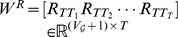 , we have
  .
.
Proof
With Proposition 1 and Definition 2, we know there's a temporal tree  of each
  in TOG, and each
  is a leading tree when compared with
  (refer to the definition of BFS spanning tree with the TOG model). Therefore, each temporal tree
  is a leading tree when compared with
  . Two strategies are adopted to yield a leading temporal tree: i) Adding new nodes into
  , i.e., we have
  , ii) Adding new paths to the existing nodes, i.e., we have
  . In the case of strategy i), if there's only one temporal tree, we obviously have
  ; if the number of temporal trees is
  , and
, and  , then when the number of temporal trees is
  , we have
 , where (
 ) denotes a nonzero vector. In the case of strategy ii), each new interaction in leading tree
  , which isn't included in temporal tree
  , contributes to new paths to the existing nodes. By some linear superposition of columns of matrix
  and
and  , we find there's no impact on the maximum rank of matrix
  if we cut down and drop those “old” interactions, which means we only need to take the leading temporal tree, i.e.
  , into consideration. Therefore, we have
  , where
  ,
,  ,
,  and
and  are properly defined linear transformation matrices.
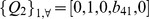
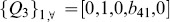
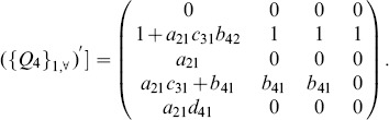
For example, according to Definition 2, the reachability of temporal tree  of Fig. 3 (c) is
  . Similarly, we have
  ,
,  and
and 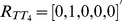 for temporal trees
  ,
,  and
and  , respectively. Therefore, we easily reach
  , and
, and 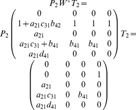 .Obviously,
  , which is consistent with Proposition 2.
Definition 3
Temporal trees  are homogeneously structured if their corresponding adjacency matrices, denoted as
  , are same structured. Otherwise, they are heterogeneously structured.
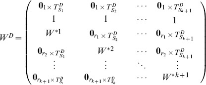
We rewrite matrix  as:
as:
| (9) |
In Eq. (9), matrix  of size
  denotes the part of heterogeneously structured trees, and matrix
  of size
  denotes the part of homogeneously structured trees, respectively. Obviously,
  .
.
2.2.1 Heterogeneously Structured Trees
Definition 4
If heterogeneous trees  consist of same nodes, i.e.,
  , then they are called heterogeneous trees with same nodes. Otherwise they are heterogeneous trees with different nodes.
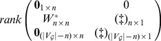
To determine the rank of matrix  , we rewrite it as:
 |
(10) |
In Eq. (10), each  ,
,  , of size
  denotes a collection of heterogeneous trees with same nodes (
 for
for  ), and
  of size
  denotes heterogeneous trees with different nodes.
  .
.
Case 1
Heterogeneous trees with same nodes.
Proposition 3
Given matrix  as a collection of heterogeneous trees with same nodes, we have
  ,
,  , where
  denotes the number of nodes in matrix
  .
.
Proof
According to the definition of heterogeneous trees with same nodes, these trees always have the same reachability with different paths to reach the same node, which means for each heterogeneously structured temporal tree with same nodes, there exists at least one independent parameter (interaction). When  ,
,  . When
  , we get a triangular matrix with its diagonal elements non-zeros by some linear transformations. Therefore, we have
  . Similarly, when
  , we get
  . In short, we reach
  .
.
Case 2
Heterogeneous trees with different nodes.
Proposition 4
Given matrix  as heterogeneous trees with different nodes, we have
  .
.
Proof
When  , we easily have
  . If
. If  , and
, and  , then when
  , it's equivalent to add a tree with different nodes into matrix
  to get matrix
  . Therefore, there always exists at least one new nonzero entry with its column index
  and row index
  in matrix
  , and
, and 
 , where (
 ) denotes a nonzero vector. That means for any
  , we have
 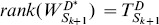 . Note that if we cannot find such a nonzero entry, we claim that this new tree must have a collection of nodes coincident to some other tree, which is not allowed in this case.
Theorem 1
Given matrices  ,
,  , as the heterogeneously structured trees and
  as the maximum-structurally controllable subspace of heterogeneously structured trees, we have
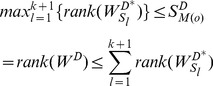 |
(11) |
Proof
Firstly, we prove the left part of inequality (11), i.e.  . Compared with the trees, denote as
  , in matrix
  (
( ), those trees in matrices
  have different nodes, i.e.,
  , and
, and  for
for  . Therefore,
  when there exists a matrix consists of all nodes, and it has the maximum rank. For the right part, i.e.
 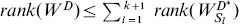 , we reach the equality when matrix
  is written as:
 , where row vector
  , i.e, the
  row of matrix
  , denotes node
  , and matrices
  denote the other part of these trees. This means there's no intersection of nodes between any two matrices of
  except node
  , i.e.,
  for
for  . In this case, each matrix
  contributes
  to
to  . Therefore,
  .
.
2.2.2 Homogeneously Structured Trees
Definition 5
Consider homogeneously structured trees  . If their corresponding adjacency matrices
  are independent, then they are called independent trees. Otherwise they are interdependent trees.
We rewrite matrix  as:
as:
| (12) |
and each  denote a collection of homogeneously structured trees (
 for
for  ), which is written as:
 |
(13) |
In Eq. (13), each  ,
,  , of size
  denotes a collection of interdependent trees with same interactions (
 for
for  , where
  denotes the collection of same interactions in matrix
  ), and
  of size
  denotes independent trees. For homogeneously structured trees, we have
  and
and  ,
,  , where
  and
and  denote the number of nodes in matrices
  and
and  , respectively.
Case 1
Independent trees.
Proposition 5
Given matrix  as independent trees, we have
  , where
  denotes the number of nodes in matrix
  .
.
Proof
According to the definition of independent matrices, the matrix having the reachability vectors of independent trees from the controller  , i.e.
  , is a structured matrix. For such a structured matrix, we can always find a square sub-matrix of size
  , whose elements are all non-zero. Therefore, it's obvious that
  .
.
An illustrative example is given with Fig. 4 (a). The corresponding matrix  is written as:
  , whose rank is 2, i.e.,
  . More generally, if
  , matrix
  is written as:
 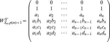 and
and  .
.
Figure 4. Three examples of the homogeneously structured temporal trees.

(a) Independent trees, (b) and (c) Interdependent trees. For the two homogeneously structured trees in (b), there are three same interactions, i.e (B,C,5), (B,D,5) and (B,E,5), but there are only two such interactions, i.e (B,C,5) and (B,D,5), for the trees in (c). The trees in (b) and (c) are both interdependent according to our definition. The numbers in parenthesis denote active time points of interactions and characters  denote the weights of interactions.
Case 2
Interdependent trees.
Proposition 6
Given matrix  as a collection of interdependent trees, we have
 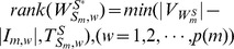 , where
  denotes the number of nodes, and
  is the number of same interactions in
  .
.
Proof
Without loss of generality, we firstly prove the case of two trees as shown in Fig. 4 (b). Here  , i.e. interaction
  and
and  . The corresponding matrix
  , and it's obvious that the dependence of elements in matrix is caused by the interdependent of trees in some interactions. Thus
  . More generally, when extending to the case of
  trees,
  , and
, and  . Similarly, for the trees in Fig. 4 (c),
  , and
, and  . Similarly, when extending to the case of
  trees,
  , and
, and  .
.
Theorem 2
Given matrices  ,
,  , as homogeneously structured trees, we have
 |
(14) |
where  is the number of nodes, and
  is the number of same interactions in
  ,
,  .
.
Proof
The outsider function  ensures that the rank of matrix
  never exceeds the number of independent rows, i.e., the number of nodes in matrix
  . Next we focus on the number of independent columns. From the proof of Proposition 5, we know there always exists a structured square matrix of size
  in matrix
  , so there always exists
  independent columns compared with interdependent matrix
  , which means matrix
  always contributes
  to matrix
  , i.e.,
  in Eq. (14). Now we focus on the part of
 , which deals with the rank of all interdependent trees, i.e. the rank of matrix
  . Without loss of generality, for trees shown in Fig. 4 (b) and (c), we have
  ,and
,and  . More generally, when extending to the case of
  trees, we similarly have
 . When
  , it's easy to verify that
  . So the rank of matrix
  is
is  .
.
With Eq. (12) and Theorem 2, we directly give the following Lemma 1 for homogeneously structured trees.
Lemma 1
Given matrices  ,
,  , as collections of homogeneously structured trees and
  as the maximum-structurally controllable subspace of homogeneously structured trees, we have
| (15) |
With Theorem 1, Theorem 2 and Lemma 1 above, we straightly get Theorem 3:
Theorem 3
Given  and
and  as the maximum controlled subspace of heterogeneously structured and homogeneously structured temporal trees in Eq. (11) and (15), respectively, we have
| (16) |
2.3 Numerical Simulations
We firstly verify the feasibility and reliability of Theorem 3. As shown in Fig. 5, four different networks with sizes of 40, 60, 80 and 100 are studied, respectively. For each of the four networks, we randomly generate an interaction between a pair of nodes with probability 0.002, and repeat it for all the  pairs of nodes at a specified time point. Repeat this process for 100 rounds at 100 different time points, i.e.
  . As shown in Fig. 5, all the calculated values of controlling centrality of the four networks (denoted as 'Calculated') are between the upper and lower bounds (denoted as 'Upper Bound' and 'Lower Bound', respectively) given by our analytical results in Eq. (16). Besides, the gaps (numerical calculations) between upper and lower bounds are very minor in these artificial networks.
Figure 5. Controlling centrality of artificial networks.

(a), (b), (c) and (d) denote network with 40, 60, 80 and 100 nodes, respectively. For each of the four networks, we randomly generate an interaction between a pair of nodes with probability 0.002, and repeat it for all the  pairs of nodes at a specified time point. repeat this process for 100 rounds at 100 different time points, i.e.
  . The value of controlling centrality, denoted as 'Calculated', is straightly calculated by the computation of matrix
  in Eq. (19), and the upper and lower bounds, denoted as 'Upper Bound' and 'Lower Bound', respectively, are given by the analytical results in Eq. (16).
We further investigate three empirical datasets, i.e., 'HT09', 'SG-Infectious' and 'Fudan WIFI' (Details of the datasets see Methods) [31], [35], [36], [43]. For the dataset of 'HT09', two temporal networks are generated: i) a temporal network (113 nodes and 9865 interactions) with all nodes and interactions within record of dataset, denoted as 'all range', ii) a temporal network (73 nodes and 3679 interactions) with nodes and interactions after removing the most powerful nodes (nodes with the largest controlling centrality) in the temporal network of i), denoted as 'removed'. For the dataset of 'SG-Infectious', three temporal networks are generated: i) a temporal network (1321 nodes and 20343 interactions) with nodes and interactions recorded in the first week, denoted as 'Week 1', ii) a temporal network (868 nodes and 13401 interactions) with nodes and interactions recorded in the second week, denoted as 'Week 2', iii) a temporal network (2189 nodes and 33744 interactions) with nodes and interactions recorded in the first two weeks, denoted as 'Week 1&2'. For the dataset of 'Fudan WIFI', three temporal networks are generated: i) a temporal network (1120 nodes and 12833 interactions) with nodes and interactions recorded in the first day, denoted as 'Day 1', ii) a temporal network (2250 nodes and 25772 interactions) with nodes and interactions recorded in the second day, denoted as 'Day 2', iii) a temporal network (1838 nodes and 27810 interactions) with nodes and interactions recorded at Access Point No. 713, denoted as '713 point'. With these three types of eight temporal networks, we calculate their upper and lower bounds of controlling centrality given by our analytical results (it's difficult to directly calculate the rank of matrix  for large-scale networks). The aggregated degree of a node in Figs. 6 and 7 is the number of neighbored nodes whom it interacts within the corresponding temporal network. As shown in Fig. 6, although the sizes of these networks range from 73 to 2250, the gaps of the upper and lower bounds remain very tiny, indicating the feasibility and reliability of Eq. (16) in both artificial (refer to Fig. 5) and empirical networks. Fig. 7 shows us the positive relationship between the aggregated degree and controlling centrality of nodes. When removing the most powerful nodes (nodes with the largest controlling centrality), as shown in Fig. 7 (a), and considering temporal networks with different time scales and types, as shown in Fig. 7 (b) and (c), the observed positive relationship remains unchanged. This indicates the robustness of this relationship of temporal network, regardless of the structural destructions or time evolutions of the network. Further more, Fig. 8 reveals some nodes with rather larger (smaller) controlling centrality but smaller (larger) aggregated degree, which suggests that although there's a positive relationship between aggregated degree and controlling centrality, controlling centrality is a measurement inherently different from the aggregated degree.
Figure 6. The gap of upper and lower bounds of controlling centrality.

(a) HT09 (b) SG-Infectious (c) Fudan WIFI. For the dataset of 'HT09', two temporal networks are generated: i) a temporal network (113 nodes and 9865 interactions) with all nodes and interactions within record of dataset, denoted as 'all range', ii) a temporal network (73 nodes and 3679 interactions) with nodes and interactions after removing the most powerful nodes (nodes with the largest controlling centrality) in the temporal network of i), denoted as 'removed'. For the dataset of 'SG-Infectious', three temporal networks are generated: i) a temporal network (1321 nodes and 20343 interactions) with nodes and interactions recorded in the first week, denoted as 'Week 1', ii) a temporal network (868 nodes and 13401 interactions) with nodes and interactions recorded in the second week, denoted as 'Week 2', iii) a temporal network (2189 nodes and 33744 interactions) with nodes and interactions recorded in the first two weeks, denoted as 'Week 1&2'. For the dataset of 'Fudan WIFI', three temporal networks are generated: i) a temporal network (1120 nodes and 12833 interactions) with nodes and interactions recorded in the first day, denoted as 'Day 1', ii) a temporal network (2250 nodes and 25772 interactions) with nodes and interactions recorded in the second day, denoted as 'Day 2', iii) a temporal network (1838 nodes and 27810 interactions) with nodes and interactions recorded at Access Point No. 713, denoted as '713 point'. The upper and lower bounds of the controlling centrality are given by analytical results in the main text, and the gap is given by the absolute value of the difference of the upper and lower bounds. The aggregated degree of a node is the number of neighbored nodes whom it interacts within the corresponding temporal network. All the gaps are minor when compared with the sizes of these temporal networks.
Figure 7. The statistical relationship between node's aggregated degree and the average controlling centrality.

(a) HT09 (b) SG-Infectious (c) FudanWIFI. All the temporal networks are the same as those in Fig. 6. Each point in this figure is an average controlling centrality of nodes with the same aggregated degree, and there's a positive relationship between the aggregated degree and its controlling centrality, even with some structural destructions or time evolutions.
Figure 8. The specific relationship between node's aggregated degree and controlling centrality.

(a) and (b) Temporal networks generated by the dataset of 'SG-Infectious' (c) and (d) Temporal networks generated by the dataset of 'Fudan WIFI'. Although big nodes (node with larger aggregated degree) tend to own larger controlling centralities, there exist many nodes with larger (smaller) aggregated degree but smaller (larger) controlling centrality, such as circled points in (a), (b) and (d).
Besides, Fig. 9 focuses on the datasets of 'SG-Infectious' and 'Fudan WIFI' to visualize the distribution of controlling centrality of different temporal networks. The scale-free distribution of node's controlling centrality is virtually independent of the time period and network scale, which is similar to the distribution of node's activity potential [47]. However, these two studied datasets are inherently different. The dataset of 'SG-Infectious' collected the attendee's temporal activity information during an exhibition, where the attendee generally do not appear again after the visit. Therefore, the interactions among nodes in the temporal networks generated from 'SG-Infectious' present more randomness than those of 'Fudan WIFI', while the latter presents weekly rhythm of the scheduled campus activities in a university.
Figure 9. The distribution of node's controlling centrality.

(a) Temporal networks generated by the dataset of 'SG-Infectious' (b) Temporal networks generated by the dataset of 'Fudan WIFI'. For each dataset, three different temporal networks are generated within different time scales, denoted as 'Week 1', 'Week 2' and 'Week 1&2' for SG-Infectious and 'Day 1', 'Day 2' and '713 point' for Fudan WIFI, respectively.
Discussion
Many problems on networks involving time are raised by some common themes, especially on communication in distributed networks, epidemiology and scheduled transportation networks. In some earlier literatures, authors studied a model with each edge of a graph associating with a single active time point (or equivalently a single starting and ending time points). So each edge has a reaction time, i.e. the delay, to transmit an information to the other end of the edge. This simple model had raised a number of interesting open questions about the basic properties of the original graph. However, such a simplified model is far enough for the cases in our information society, where relationships are varying, they are strengthened or weakened, even disappeared or created, and the exchange of information happens frequently, i.e. a pair of node exchanges information for far more than just once. Although, with the record of temporal networks being available by digital technologies, many attentions have been attracted to this area [37], little work has been carried out on the structural controllability.
In this paper, we propose a framework from graphic perspective to address the structural controllability of temporal networks, especially focusing on the ability of a single node to control the whole network (controlling centrality), which allows us analyzing large-scale networks more convenient and efficient. Noting that the single node here does not necessarily to be driven node as the one in the seminal paper of Liu et al. [12], it is randomly chosen from the whole network and we mainly focus on its controlling centrality – a measurement of its importance from the perspective of control theory. Although there's a positive relationship between controlling centrality and aggregated degree, these two centralities are obviously not equivalent in neither definition nor methodology. Frankly, more steps can be taken on the structural controllability of temporal networks in the near future. For example, one of opening problems, untouched in this paper and waiting for endeavor studies and explorations elsewhere, is the multi-inputs case. Whether or not the LTV framework still suitable for the analysis, we are looking forward for the answers.
Methods
4.1 Notation
The symbols used in the main text are summarized in Table 2.
Table 2. Notations in the paper.
| Notations | Description |

|
the  formation of temporal network formation of temporal network 
|
 and and 
|
the set of nodes and the cardinality of set 
|

|
the adjacency matrix of graph 
|

|
the transpose of adjacency matrix 
|

|
the  power of adjacency matrix power of adjacency matrix 
|

|
an element of matrix  with position with position  (row index) and (row index) and  (column index) (column index) |

|
the  row of matrix row of matrix 
|

|
the controller located on node  of temporal network of temporal network 
|

|
dynamic communicability matrix of temporal network  at time at time 
|

|
reachability matrix of input signal within the temporal network 
|

|
reachability vector of input signal within a temporal tree 
|

|
reachability vector of input signal within heterogeneously structured |
temporal tree 
|
|

|
reachability vector of input signal within homogeneously structured |
temporal tree 
|
|

|
reachability matrix of input signal within temporal trees extracted from |
temporal network 
|
|

|
reachability matrix of input signal within heterogeneously structured |
| temporal trees | |

|
reachability matrix of input signal within homogeneously structured |
| temporal trees | |

|
the maximum controlled subspace of temporal network 
|
with single controller located on 
|
|

|
the maximum controlled subspace of heterogeneously structured |
temporal trees with single controller located on 
|
|

|
the maximum controlled subspace of homogeneously structured |
temporal trees with single controller located on 
|
4.2 Controlling Centrality
With a sampling interval properly chosen, we write Eq. (3) as follow:
| (17) |
Generally,  , where
  is the sampling interval. From Eq. (17), we get the recursive relationship of two neighboring states as:
| (18) |
Where 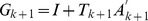 ,
,  ,
,  and
and  are the transpose of the adjacency matrix of the
  th graph and the identity matrix, respectively. Define
| (19) |
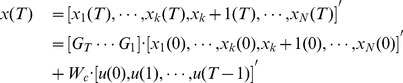
and the final state is written as:
 |
(20) |
If there exists a sequence of inputs denoted as  such that
  in Eq. (20), then the temporal network is structurally controllable at time point
  , i.e.
  . Otherwise, we may split
  into two parts, written as:
 |
(21) |
and if there exists a sequence of inputs denoted as  such that
  in Eq. (21), then the
  subspace of the network is structurally controllable at time point
  , which is equivalent to the condition
  . Therefore, we define controlling centrality as
| (22) |
i.e. the maximum dimension of controllable subspace, as a measure of node  's ability to structurally control the network: if
  , then node
  alone can structurally control the whole network. Any value of
  less than
  provides the maximum dimension of the subspace
  can structurally control.
4.3 Datasets
We mainly investigate three temporal networks with three empirical data sets in this paper. The first data was collected during the ACM Hypertext 2009 conference, where the 'SocioPatterns' project deployed the Live Social Semantics applications. The conference attendees volunteered to wear radio badges which monitored their face-to-face interactions and we name this data as 'HT09'. The second is a random data set containing the daily dynamic contacts collected during the art-science exhibition 'INFECTIOUS: STAY AWAY' which took place at the Science Gallery in Dublin, Ireland, and we name it as 'SG-Infectious'. These two data are both available from the website of 'SocioPatterns' [31] (http://www.sociopatterns.org). The third data set was collected from Fudan University during the 2009-2010 fall semester (3 whole months), which is named as 'FudanWIFI' [35], [36], [43]. In this data set, each student/teacher/visiting scholar has a unique account to access the Campus WiFi system, which automatically records the device' MAC addresse, the MAC address of the accessed WiFi access point (APs), and the connecting (disconnecting) time as well. Table 3 summaries some characteristics of the aforementioned three empirical datasets.
Table 3. Characteristics of the three empirical datasets.
| HT09 | SG-Infectious | FudanWIFI | |
| Area | Conference | Mesume | Campus |
| Technology | RFID | RFID | WiFi |
| Collection | 3 days | 62 days | 84 days |
| duration | |||
| Number of | 113 | 10970 | 17897 |
| individuals | |||
| Number of | 9865 | 198198 | 884800 |
| contacts | |||
| Spatial |
 2 2 |
 2 2 |
 8 8 |
| resolution(meters) | |||
| Types of | Strangers | Acquaintances | Acquaintances |
| contacts | with repeat | without repeat | with repeat |
Funding Statement
This work was partly supported by National Key Basic Research and Development Program (No. 2010CB731403), the National Natural Science Foundation (No. 61273223), the Research Fund for the Doctoral Program of Higher Education (No. 20120071110029) and the Key Project of National Social Science Fund (No. 12&ZD18) of China. The funders had no role in study design, data collection and analysis, decision to publish, or preparation of the manuscript.
References
- 1. Watts DJ, Strogatz SH (1998) Collective dynamics of small-world networks. Nature 393: 440–442. [DOI] [PubMed] [Google Scholar]
- 2. Barabási AL, Albert R (1999) Emergence of scaling in random networks. Science 286: 509–512. [DOI] [PubMed] [Google Scholar]
- 3. Albert R, Barabási AL (2002) Statistical mechanics of complex networks. Rev Mod Phys 74: 47–97. [Google Scholar]
- 4.Newman M, Barabási AL, Watts DJ (2006) The Structure and Dynamics of Networks. Princeton Univ Press.
- 5. Wang XF, Chen GR (2002) Pinning control of scale-free dynamical networks. Physica A 310: 521–531. [Google Scholar]
- 6. Li X, Wang XF, Chen GR (2004) Pinning a complex dynamical network to its equilibrium. IEEE Trans Circ Sys I 51: 2074–2087. [Google Scholar]
- 7. Li X, Wang XF (2006) Controlling the spreading in small-world evolving networks: Stability, oscillation, and topology. IEEE Trans Automat Contr 51: 534–540. [Google Scholar]
- 8. Yu WW, Chen GR, Lü JH (2009) On pinning synchronization of complex dynamical networks. Automatica 45: 429–435. [Google Scholar]
- 9. Rahmani A, Ji M, Mesbahi M, Egerstedt M (2009) Controllability of multi-agent systems from a graphtheoretic perspective. SIAM J Contr Optim 48: 162–186. [Google Scholar]
- 10. Gutiérrez R, Sendiñ-Nadal I, Zanin M, Papo D, Boccaletti S (2012) Targeting the dynamics of complex networks. Sci Rep 2: 396. [DOI] [PMC free article] [PubMed] [Google Scholar]
- 11. Lombadi A, Hörnquist M (2007) Controllability analysis of networks. Phys Rev E 75: 056110. [DOI] [PubMed] [Google Scholar]
- 12. Liu YY, Slotine JJ, Barabási AL (2011) Controllability of complex networks. Nature 473: 167–173. [DOI] [PubMed] [Google Scholar]
- 13. Wang WX, Ni X, Lai YC, Grebogi C (2012) Optimizing controllability of complex networks by minimum structural perturbations. Phys Rev E 85: 026115. [DOI] [PubMed] [Google Scholar]
- 14. Liu YY, Slotine JJ, Barabási AL (2012) Control centrality and hierarchical structure in complex networks. PLoS ONE 7: e44459. [DOI] [PMC free article] [PubMed] [Google Scholar]
- 15. Nepusz T, Vicsek T (2012) Controlling edge dynamics in complex networks. Nat Phys 8: 568–573. [Google Scholar]
- 16. Yan G, Ren J, Lai YC, Lai CH, Li B (2012) Controlling complex networks: How much energy is need? Phys Rev Lett 108: 218703. [DOI] [PubMed] [Google Scholar]
- 17. Cowan NJ, Chastain EJ, Vilhena DA, Freudenberg JS, Bergstrom CT (2012) Nodal dynamics, not degree distributions, determine the structural controllability of complex networks. PLoS ONE 7: e38398. [DOI] [PMC free article] [PubMed] [Google Scholar]
- 18. Pósfai M, Liu YY, Slotine JJ, Barabási AL (2013) Effect of correlations on network controllability. Sci Rep 3: 1067. [DOI] [PMC free article] [PubMed] [Google Scholar]
- 19. Delpini D, Battiston S, Riccaboni M, Gabbi G, Pammolli F, Caldarelli G (2013) Evolution of controllability in interbank networks. Sci Rep 3: 1626. [DOI] [PMC free article] [PubMed] [Google Scholar]
- 20. Sun J, Motter AE (2013) Controllability transition and nonlocality in network control. Phys Rev Lett 110: 208701. [DOI] [PubMed] [Google Scholar]
- 21. Jia T, Barabási AL (2013) Control capacity and a random sampling method in exploring controllability of complex networks. Sci Rep 3: 2354. [DOI] [PMC free article] [PubMed] [Google Scholar]
- 22. Kalman RE (1963) Mathematical description of linear dynamical systems. J Soc Indus Appl Math Ser A 1: 152–192. [Google Scholar]
- 23.Luenberger DG (1979) Introduction to Dynamic Systems: Theory, Models, & Applications. Wiley Press.
- 24.Slotine JJ, Li W (1991) Applied Nonlinear Control. Pretice-Hall Press.
- 25. Lin CT (1974) Structural controllability. IEEE Trans Automat Contr 19: 201–208. [Google Scholar]
- 26. Shields R, Pearson J (1976) Structural controllability of multiinput linear systems. IEEE Trans Automat Contr 21: 203–212. [Google Scholar]
- 27. Hosoe S (1980) Determination of generic dimensions of controllable subspaces and its application. IEEE Trans Automat Contr 25: 1192–1196. [Google Scholar]
- 28. Mayeda H (1981) On structural controllability theorem. IEEE Trans Automat Contr 26: 795–798. [Google Scholar]
- 29. Poljak S (1989) Maximum rank of powers of a matrix of a given pattern. Proc Amer Math Soc 106: 1137–1144. [Google Scholar]
- 30. Poljak S (1990) On the generic dimension of controllable subspaces. IEEE Trans Automat Contr 35: 367–369. [Google Scholar]
- 31. Isella L, Stehlé J, Barrat A, Cattuto C, Pinton JF, et al. (2011) What's in a crowd? Analysis of face-to-face behavioral networks. J Theor. Biol 271: 166–180. [DOI] [PubMed] [Google Scholar]
- 32. Takaguchi T, Sato N, Yano K, Masuda N (2012) Importance of individual events in tenporal networks. New J Phys 14: 093003. [Google Scholar]
- 33. Barabási AL (2005) The origin of bursts and heavy tails in human dynamics. Nature 435: 207–211. [DOI] [PubMed] [Google Scholar]
- 34. González MC, Hidalog CA, Barabási AL (2008) Understanding individual human mobility patterns. Nature 453: 779–782. [DOI] [PubMed] [Google Scholar]
- 35. Zhang Y, Wang L, Zhang YQ, Li X (2012) Towards a temporal network analysis of interactive WiFi users. Europhys Lett 98: 68002. [Google Scholar]
- 36. Zhang YQ, Li X (2013) Temporal dynamics and impact of event interactions in cyber-social populations. Chaos 23: 013131. [DOI] [PubMed] [Google Scholar]
- 37. Holme P, Saramäki J (2012) Temporal networks. Phys Rep 519: 97–125. [Google Scholar]
- 38. Kostakos V (2009) Temporal graphs. Physica A 388: 1007–1023. [Google Scholar]
- 39. Kim H, Anderson R (2012) Temporal node centrality in complex networks. Phys Rev E 85: 026107. [DOI] [PubMed] [Google Scholar]
- 40. Grindrod P, Parsons MC, Higham DJ, Estrada E (2011) Communicability across evolving networks. Phys Rev E 83: 046120. [DOI] [PubMed] [Google Scholar]
- 41. Perra N, Baronchelli A, Mocanu D, Gonçalves B, Pastor-Satorras R, et al. (2012) Random walks and search in time-varying networks. Phys Rev Lett 109: 238701. [DOI] [PubMed] [Google Scholar]
- 42. Tang J, Scellato S, Musolesi M, Mascolo C, Latora V (2010) Small-world behavior in time-varying graphs. Phys Rev E 81: 055101. [DOI] [PubMed] [Google Scholar]
- 43. Zhang YQ, Li X (2012) Characterizing large-scale population's indoor spatio-temporal interactive behaviors. Proc ACM SIGKDD Int Workshop on Urban Computing (UrnComp' 12): 25–32. [Google Scholar]
- 44. Nicosia V, Tang J, Musolesi M, Russo G, Mascolo C, et al. (2012) Components in time-varying graphs. Chaos 23: 023101. [DOI] [PubMed] [Google Scholar]
- 45.Ribeiro B, Perra N, Baronchelli A (2012) Quantifying the effect of temporal resolution on time-varying networks. ArXiv:1211.7052. [DOI] [PMC free article] [PubMed]
- 46. Krings G, Karsai M, Bernhardsson S, Blondel VD, Saramäki J (2012) Effects of time window size and placement on the structure of an aggregated communication network. EPJ Data Science 1: 4. [Google Scholar]
- 47. Perra N, Gonçalves B, Pastor-Satorras R, Vespignani A (2012) Activity driven modeling of time varying networks. Sci Rep 2: 469. [DOI] [PMC free article] [PubMed] [Google Scholar]