Deoxygenation of the Baltic Sea during the last century

Significance

Oxygen-deficient waters are expanding globally in response to warming and coastal eutrophication. Coastal ecosystems provide valuable services to humans, but these services are severely reduced with decreasing oxygen conditions. In the Baltic Sea, oxygen-deficient waters have expanded from 5,000 to over 60,000 km² with large decadal fluctuations over the last century, reducing the potential fish yield and favoring noxious algal blooms. This increase is due to the imbalance between oxygen supply from physical processes and oxygen demand from consumption of organic material, enhanced by nutrient inputs and temperature increases. Further nutrient reductions will be necessary to restore a healthier Baltic Sea and counteract effects from warming.

Abstract

Deoxygenation is a global problem in coastal and open regions of the ocean, and has led to expanding areas of oxygen minimum zones and coastal hypoxia. The recent expansion of hypoxia in coastal ecosystems has been primarily attributed to global warming and enhanced nutrient input from land and atmosphere. The largest anthropogenically induced hypoxic area in the world is the Baltic Sea, where the relative importance of physical forcing versus eutrophication is still debated. We have analyzed water column oxygen and salinity profiles to reconstruct oxygen and stratification conditions over the last 115 y and compare the influence of both climate and anthropogenic forcing on hypoxia. We report a 10-fold increase of hypoxia in the Baltic Sea and show that this is primarily linked to increased inputs of nutrients from land, although increased respiration from higher temperatures during the last two decades has contributed to worsening oxygen conditions. Although shifts in climate and physical circulation are important factors modulating the extent of hypoxia, further nutrient reductions in the Baltic Sea will be necessary to reduce the ecosystems impacts of deoxygenation.

Dead zones are hypoxic (low-oxygen) areas unable to support most marine life, and over the past 50 y they have spread rapidly in the open ocean (1) as well as in coastal ecosystems (2). Global warming is thought to be a major driver for these changes (3), although biogeochemical factors have also been recognized, especially in coastal marine ecosystems (4, 5). In the Baltic Sea, the present spread of hypoxia is the combined result of climate changes influencing deepwater oxygenation (6) and increased eutrophication (7, 8), resulting in a hypoxic area ranging between 12,000 and 70,000 km² with an average of 49,000 km² over the time period 1961–2000 (7). Here, we separate the effects of the two factors on oxygen conditions.

Physical factors are an important consideration in whether an ecosystem will experience hypoxia. The Baltic Sea is naturally prone to hypoxia due to a restricted water exchange with the ocean and a long residence time above 30 y (9, 10). Saltier, denser water from the North Atlantic flows over a series of shallow sills in the Danish Straits to ventilate waters below the permanent halocline and are governed by meteorological-induced variations in sea levels (11), displaying variations at decadal scales (12, 13). The dense saltwater inflows bring new supplies of oxygen to bottom waters, but at the same time enhance stratification, creating larger bottom areas that experience hypoxia (14). In particular, the ventilation of the deeper waters is attributed to events of larger inflows of high-saline water (>17), termed Major Baltic Inflows (MBIs), that have been less frequent in the last three decades (6).

Climate warming decreases oxygen solubility due to higher water temperature, increases stratification, and enhances respiration processes (15). Climate warming is likely to be accompanied by increased precipitation and inflows of freshwater and nutrients to coastal waters in many areas of the globe. Increasing nutrient inputs from land stimulates primary production and export of organic material to the deep waters, thereby disrupting the subtle natural balance between oxygen supply from physical processes and oxygen demand from consumption of organic material. However, the importance of decreasing oxygenation versus increasing nutrient inputs for explaining the recent spread of hypoxia is not known (6, 7).

Water column measurements of dissolved oxygen concentrations began around 1900 with more regularly spaced measurements commencing in the 1960s (Fig. S1), allowing a more consistent assessment of the spatial extent of hypoxia (7, 14). The sparse temporal and spatial resolution of oxygen data before 1960 allowed only assessing hypoxia at specific locations (16) or specific years (17). To our knowledge, our study is the first to report basin-wide trends of stratification and oxygen conditions from 1898 to present, and here we will focus on the two basins that have perennial hypoxia—the Bornholm Basin and the Gotland Basin (Fig. S2). These two basins are connected via a channel with a sill depth of 60 m.

Results

Over the past century, bottom-water temperatures increased about 2 °C in both basins (Fig. 1 A and B), whereas bottom-water salinity exhibited multidecadal oscillations without trends, displaying larger and more dynamic variations in the Bornholm Basin that has a shorter residence time than the Gotland Basin (Fig. 1 C and D). Periods of intense saltwater inflows, such as around 1950 (12), increased salinity of the bottom water by ∼1. Saltwater inflows were weak from 1982 to 1993, termed the stagnation period (12), which resulted in a freshening of both bottom (Fig. 1 C and D) and surface waters (Fig. S3), although the surface water response in the Gotland Basin was delayed. The deepwater temperature also decreased during the stagnation period (Fig. 1B), due to less inflow of warmer water from the Danish Straits. In the Gotland Basin, the halocline gradually deepened from 70 to 80 m (Fig. 1 E and F), an unprecedented low position of the halocline within the 20th century. The lower depth of the discontinuity layer was similarly displaced from 85 to 100 m (Fig. S3), resulting in much deeper mixing across the halocline. In the Bornholm Basin, the position of the halocline was relatively constant, because it is largely controlled by the sill depth of the connecting channel. The freshening of the bottom water, combined with a delayed response of surface salinity, reduced stratification strength during the stagnation period enabling mixing across the halocline, most pronounced for the Gotland Basin (Fig. 1 G and H). Overall, the properties of the halocline remained relatively constant since 1900, with the exception of the stagnation period.

Fig. 1.

Long-term trends in temperature, salinity, and oxygen characteristics. The left panel show trends for the Bornholm Basin, and the right panel show trends for the Gotland Basin. Trends are temperature in the bottom layer (A and B), bottom-water salinity (C and D), depth location of the halocline (E and F), Brunt–Väisälä frequency, which is a proxy for stratification strength, calculated from the salinity profile parameters (G and H), apparent oxygen utilization (AOU) at the lower boundary of the discontinuity layer (I and J), change in AOU with depth below the discontinuity layer (K and L), areal extent of hypoxia (<2 mg⋅L⁻¹) with the bottom area below the discontinuity layer (M and N), and total AOU below the discontinuity layer (O and P). The circles represent annual means and the solid black line is the 5-y moving average. A few outliers are not shown in the plots above but can be seen in Fig. S3 together with SEs of the annual means. Seasonal and spatial distributions of profile parameters are shown in Figs. S4 and S5.

Climate change has caused the bottom waters to become increasingly oxygen depleted through decreasing solubility of oxygen due to increasing temperature and through increased respiration of organic matter. Oxygen saturation has decreased about 0.5 mg⋅L⁻¹ over the past 115 y as a result of the temperature increase alone. In addition, apparent oxygen utilization (AOU), a measure of the deoxygenation (see definition in Data and Methods), at the lower boundary of the discontinuity layer increased gradually by 2 and 4 mg⋅L⁻¹ in the Bornholm Basin and Gotland Basin, respectively (Fig. 1 I and J), although with a marked decrease in the Gotland Basin during the stagnation period. AOU further decreased below the discontinuity layer at a relatively constant slope over time of 0.15 mg⋅L⁻¹⋅m⁻¹ in the Bornholm Basin (Fig. 1K) and with a substantially lower slope around 0.025 mg⋅L⁻¹⋅m⁻¹ in the Gotland Basin, albeit displaying a doubling during the stagnation period (Fig. 1L). The strongly oxygen-depleted waters were confined to the deepest parts of the Gotland Basin, where high concentrations of hydrogen sulfide were observed, and did not spread due to lack of MBI events. The time series also suggest that a minor stagnation period could have occurred around 1930 with decreasing salinity (Fig. 1D), lower AOU below the discontinuity layer (Fig. 1J), and increasing slope of AOU with depth (Fig. 1L), consistent with a reported 3-y period without any MBI (12).

The area of hypoxia (here, oxygen concentrations <2 mg⋅L⁻¹) expanded in both basins (Fig. 1 M and N), increasing from around 5,000 km² to over 60,000 km² over the past 115 y. In the beginning of the 20th century, hypoxia was confined to the deepest areas (Fig. 2A), expanding gradually over the next 70 y (Fig. 2 B–D), before the extent decreased during the stagnation period. At the end of the stagnation period, hypoxia had approximately the same extent as in 1931 (Fig. 2 B and E), but hypoxia has spread again over the last two decades, reaching an unprecedented large extent in recent years (Fig. 2F). In the Gotland Basin, the extent of hypoxia is increasingly controlled by the bottom area below the discontinuity layer, and now almost the entire area below the discontinuity layer is hypoxic (Fig. 1N). In the Bornholm Basin, the hypoxic bottom water is occasionally flushed into the Gotland Basin during strong MBI events, most pronounced in 1993 and 2003 (Fig. 1M). Such inflows typically amount to 150–300 km³ with the potential to improve the total AOU (TAOU) by ∼1–2 10¹² g O₂, provided that the Bornholm Basin deep waters are completely flushed. The two above-mentioned MBIs actually improved the TAOU by ∼0.5 10¹² g O₂ (Fig. 1O), but the export of this hypoxic water was not apparent in the AOU balance for the Gotland Basin (Fig. 1P).

Fig. 2.

Spatial distributions of bottom hypoxia and anoxia over time. Estimated bottom oxygen concentrations <2 mg⋅L⁻¹ are shown in red, and concentrations <0 mg⋅L⁻¹ are shown in black for 1906 (A), 1931 (B), 1955 (C), 1974 (D), 1993 (E), and 2012 (F). The spatial distributions represent means across all months (January to December).

Our simple mass balance model demonstrates that changes in the inflow to and volume of the Gotland Basin deep waters significantly modulate oxygen conditions. Inflow and outflow generally balance, resulting in an average bottom-water volume of around 2,000 km³ (about 10% of the total volume of the Baltic Sea). However, during the stagnation period the volume of the deep waters decreased by more than 500 km³. This reduction started already around 1970 and intensified during the stagnation period (Fig. 3A). The deep-water volume increased again with the MBI in 1993, reaching the long-term average in 2000. Vertical mixing across the halocline generally had a similar order of magnitude as lateral transports and was larger than previous thought (10, 18). During the stagnation period, vertical mixing was about 50% higher.

Fig. 3.

Estimated contributions of physical processes and nutrient input to hypoxia. Water transports for the Gotland Basin deep water (A), annual fluxes of total apparent oxygen utilization (TAOU) (B), and TAOU in the deep water, estimated (5-y moving average; Fig. 1P) and adjusted by subtracting variations in lateral transports and vertical mixing (C). Nitrogen input from land and atmosphere was used to describe the oxygen consumption; similar plots using phosphorus inputs are shown in Fig. S6.

Oscillations in inflow and outflow were also apparent in the lateral imports and exports of TAOU (Fig. 3B). The export of TAOU generally exceeded import because bottom waters in the Gotland Basin were more deoxygenated than in the Bornholm Basin. However, the expansion of the deep-water volume following the stagnation period resulted in a net accumulation of TAOU from lateral transport processes. The importance of vertical mixing has increased over time due to larger differences in oxygen conditions across the halocline. The weaker stratification during the stagnation period increased the vertical mixing of oxygen by up to 30%. Oxygen consumption increased from 2.2 to 3.3 10¹² g O₂⋅y⁻¹ in the early 1980s before decreasing again. According to the budget model, only one-third of the consumption could be directly coupled to enhanced nutrient input, and only 8–25% of the input resulted in deep-water oxygen consumption (Table S1). Despite larger reductions in nutrient inputs from land and atmosphere since the 1980s (8), respiration still remains relatively high due to the increase in bottom-water temperature (Fig. 1B). In fact, warming of bottom waters following the stagnation period increased respiration by ∼20% (using estimates from Table S1). The lack of inflows significantly reduced TAOU during the stagnation period by increased vertical mixing and reduced bottom volume, but if we remove the effect of lateral transports and vertical mixing there has been a gradual increase in TAOU from around 20 to >30 10¹² g O₂ during the last century and signs of recovery are not observed (Fig. 3C).

Discussion

Climate warming plays an important role in increasing ocean deoxygenation (1), but for the Baltic Sea we show that anthropogenic nutrient discharges are the primary driving factor creating widespread hypoxic conditions. This has also been reported for other coastal ecosystems such as the Gulf of Mexico (4) and Chesapeake Bay (19), where overall increases in hypoxia from enhanced nutrient delivery are modulated by variations in freshwater inputs and stratification. The stagnation period (1982–1993) in the Baltic Sea was an exceptional event in the last 115 y, highlighting that physical forcing can remedy deoxygenation effects of eutrophication through enhanced vertical mixing. Increasing precipitation and runoff to the Baltic Sea in the 1980s is thought to be the main cause behind the lack of MBIs during the stagnation period (12). Regional climate models predict increasing river flow into the Baltic Sea (20), which, in analogy to the stagnation period, may result in a less strongly and more deeply stratified water column, alleviating hypoxia from the shoals of the deeper basins. However, increasing respiration and decreasing oxygen solubility with warming of the Baltic Sea will promote deoxygenation in the deep basins.

Substantial reductions in nutrient inputs over the last couple of decades (8) were expected to improve oxygen conditions. The apparent lack of recovery could be explained by increasing temperature and enhanced primary production by nitrogen-fixing cyanobacteria. Enhanced releases of iron-bound phosphate from sediments with expanding hypoxia (14), as observed over the last two decades, may sustain noxious cyanobacterial summer blooms, creating a positive-feedback mechanism that maintains hypoxia (21). Due to the long residence time of the Baltic Sea, elevated phosphate concentrations may still persist for decades. It is also possible that oxygen improvements anticipated from nutrient reductions have been counteracted by increases in organic matter inputs from land (22, 23). Thus, the lack of recovery could be due to delayed responses and potential hysteresis in combination with shifting baselines associated with other components of global change (24).

Hypoxia directly impacts marine ecosystem function and services through changes in food web structure and biodiversity (25, 26). Although salinity sets the limits for benthic macrofaunal diversity in the Baltic Sea and the number of functional groups is low, bottom-water hypoxia is currently the main factor structuring the benthic communities in the Gotland Basin, resulting in large areas completely devoid of macrofauna (7, 27, 28). The 10-fold increase in hypoxic area amounts to an estimated “missing” macrofaunal biomass of ∼1.7 million tons (27), with important repercussions for the transfer of energy through the food web. However, eutrophication may also stimulate secondary production in the shallower areas (29). Moreover, cod eggs are neutrally buoyant in waters with salinities between 10 and 15 and need sufficient oxygen for survival, but the volume of bottom water in the Gotland Basin possessing survivable characteristics have diminished over the last 50 y (30), threatening the reproduction of this valuable species. Thus, the large expansion of hypoxia has essentially had significant effects on the Baltic Sea ecosystem at all trophic levels.

Excessive nutrient inputs from land over the last century have altered the subtle balance between oxygen supply and consumption, from a state with hypoxia confined to the deep bottom waters to widespread hypoxia in most bottom waters. Multiple stressors and strong resilience in the Baltic Sea maintains an undesirable state with low oxygen conditions creating a positive feedback for continued hypoxia (31) supporting cyanobacteria blooms (32). Temperature increases, most prominent during the last two decades, have shifted this balance even further. Physical forcing may act to shift this balance back again, as observed during the stagnation period, but we cannot hope for future climate to counter the effects of anthropogenic pollution. Further reduction of nutrient inputs is the only realistic management option to reestablish a healthier Baltic Sea (33, 34).

Data and Methods

Study Site.

The Baltic Sea is connected to the North Sea through the entrance area consisting of the Danish Straits and the Kattegat (Fig. S2). The water exchange of the Baltic Sea is restricted by the Darss sill (15 m) and the Drogden sill (8 m) (35). The Baltic Sea consists of several connected basins. At favorable wind conditions, saline water spills over the sills and forms a bottom current in the Arkona Basin and cascades into the deeper Bornholm Basin (maximum depth, ∼90 m). From the Bornholm Basin, the bottom water enters into the larger and deeper Gotland Basin through the Słupsk Furrow, having a sill depth of 60 m. Finally, the Gotland Basin connects to the Gulf of Riga, Gulf of Finland, and Gulf of Bothnia. The Gulf of Finland can be regarded as a hydrographical extension of the Gotland Basin, and therefore these two basins are considered as one entity denoted here as the Gotland Basin.

Perennial hypoxia occurs in the Bornholm Basin and the Gotland Basin (including the Gulf of Finland) only, and the bottom layers of these two basins will be investigated in the present study. The water column in the two basins is stratified by a permanent halocline at depths around 55 and 70 m in the Bornholm Basin and Gotland Basin, respectively, and a seasonal thermocline above the halocline. Oxygen concentrations below the thermocline decline seasonally, albeit not reaching levels indicative of hypoxia, here defined as <2 mg⋅L⁻¹, but reach saturation levels again during winter when the thermocline is eroded by mixing.

Data.

Discrete and continuous depth profiles of salinity, temperature, and oxygen were obtained from national monitoring programs and research cruises (Table S2). Most profiles from before 1960 were from research cruises. The profiles were spatially scattered over the two study basins with 21,712 distinct sampling locations (Fig. S7A). Data from the coastal zone were excluded, because hypoxia in the coastal zone is not directly linked to hypoxia in the open waters (36). These many sampling locations, of which a large proportion have been sampled a few times only, were projected onto the existing monitoring network by identifying spatial clusters of sampling locations and assigning these to the nearest monitoring station. Thus, all profiles were associated with 1 out of 242 monitoring stations (Fig. S7B).

The first measurements of salinity, temperature, and oxygen in the Baltic Sea were carried out in the late 19th century, but the number of profiles before 1960 was low (Fig. S1) and these were heterogeneously sampled across the two basins considered here. The relatively lower number of profiles in the two most recent years is due to pending reporting of hydrographical measurements to the databases. A total of 36,379 salinity profiles and 16,690 oxygen profiles was sampled in the deeper areas of the two basins with permanently stratified conditions, and these profiles were used to characterize the halocline and oxygen conditions below the halocline. The reasonable data coverage after 1960 has allowed for assessing the extent of hypoxia by spatially interpolating the values (7), but such purely empirical approaches are not applicable to the period before 1960 due to the sparseness of data. Therefore, we chose an approach where we model the salinity and oxygen profiles with a few parameters, and use the spatial and seasonal structure of these parameters to assess the properties of the halocline and the oxygen conditions below the halocline from 1898 to 2012.

Parameterization of the Salinity and Oxygen Profiles.

Salinity profiles typically had a sigmoid appearance with depth and were parameterized using the cumulative probability density function of the normal distribution . Four parameters were used to characterize the salinity profile: (i) the subsurface salinity, (ii) the salinity difference between the subsurface and the bottom layer, (iii) halocline depth, and (iv) halocline thickness (Fig. S8A). The subsurface salinity (S_subsurf), estimated as the average salinity between 20 and 30 m, was used for the parameterization to avoid potential bias introduced by a thin lower-salinity layer in the surface, occasionally observed in the data. The salinity difference between the subsurface and bottom layers (S_dif) was estimated as a scaling factor for , whereas halocline depth was estimated by µ and halocline thickness was estimated as . Thus, from the properties of it is noted that 68% of the change from subsurface to bottom salinity occurs in the depth interval defined by the halocline thickness , also referred to as the discontinuity layer (37). The salinity parameters were estimated by nonlinear regression (PROC MODEL in SAS) using profiles reaching depths of at least 60 and 80 m in the Bornholm Basin and Gotland Basin, respectively, to ensure that most of the salinity change was recorded in the profile and that estimation of the profile sigmoid model was possible. The Brunt–Väisälä frequency, which can be interpreted as a measure of the stratification strength, can easily be approximated from the parameterization of the profile:

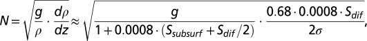where density in brackish water is approximated by salinity [ (38)] at the halocline depth in the first factor and the derivative of density with depth in the second factor is approximated by the change in salinity over the discontinuity layer.

Because the sills are shallow and inflows to the Baltic Sea occur at windy conditions, the water spilling over the Drogden and Darss sills is generally saturated in oxygen before submerging to supply the bottom waters in the study area. However, oxygen concentration at saturation varies strongly with salinity and temperature, and therefore we consider AOU, defined as the difference between the measured dissolved oxygen concentration and its equilibrium saturation concentration in water with same salinity and temperature. Hence, AOU is a measure of the oxygen consumption of the bottom water parcel since it spilled over the sills. In the last four to five decades, hydrogen sulfide (H₂S) has been measured in the deepest parts of the Gotland Basin, albeit not consistently. When measured, H₂S has been converted into a negative oxygen concentration (H₂S = −2O₂), yielding an AOU exceeding oxygen saturation concentrations. Oxidation potentials for other substances such as NH₄⁺, Fe²⁺, and Mn²⁺, were not considered. Because H₂S has not been measured consistently in the dataset and not at all before 1960, oxygen concentrations equal to zero could represent conditions with H₂S and, thus, a negative oxygen concentration and an AOU above the oxygen saturation concentration. Such observations, which actually represent values above/below their nominal values, are termed censored data (39).

In the discrete profiles, the number of oxygen measurements was generally lower than for salinity, and consequently, the parameterization of the oxygen profile had to be even simpler. Two parameters were used to characterize oxygen conditions below the halocline as a linear function of depth (Fig. S8B): (i) the AOU at the lower boundary of the discontinuity layer (intercept, AOU_boundary), and (ii) the change in AOU with depth below the discontinuity layer (slope, AOU_slope). These two parameters were estimated in two steps. First, AOU_boundary was interpolated from the nearest measured oxygen observation above and below the lower boundary of the discontinuity layer using the estimated salinity profile for interpolation rather than depth, because salinity is a better indicator of mixing than depth. The estimation of AOU_boundary was not affected by censored oxygen observations. Second, using oxygen observations below the discontinuity layer, AOU_slope was estimated by means of censored data linear regression (PROC LIFEREG in SAS) with the intercept fixed to the estimate of AOU_boundary.

Spatiotemporal Modeling of Profile Parameters.

The profiles were heterogeneously sampled in time and space, and the aim was to separate three sources of variations: (i) spatial variation, (ii) seasonal variation, and (iii) long-term trend. First, a general linear model (GLM) (PROC GLM in SAS) with station, month, and year of sampling as categorical factors was applied to each of the six parameters estimated from the salinity and oxygen profiles. Based on the station-specific means from the GLM, 2D smooth splines describing the spatial variation for each profile parameter were estimated by means of a generalized additive model (GAM) (PROC GAM in SAS). The spatial splines were used to spatially detrend all profile parameters using their actual sampling location. Second, the temporal sources of variation were estimated applying a robust GLM with two factors (month and year) on the spatially detrended observations for the two basins separately. The robust estimation algorithm, which iteratively discarded profile parameter estimates beyond the 99.9% confidence prediction interval of the GLM, was used as some measured profiles (∼5% of the profiles) delivered unrealistic parameter estimates, mostly due to lack of sufficient observations below the halocline. The second GLM provided mean estimates for the seasonal variation and long-term trend for each of the two basins separately.

The spatial models and the long-term trends for the profile parameter estimates were used for obtaining integrated values of volume, salt content, and AOU for the bottom layers of the two basins in their entirety as well as the extent of hypoxia. Yearly estimates of the profile parameters were scaled using the spatial spline model over a bathymetry grid of 1 km × 1 km (http://balance-eu.org), and salinity and oxygen profiles modeled by these parameters were integrated vertically and horizontally for the two basins separately. Thus, the time series of integrated values represent annual means for all 12 mo of the year.

Time Series Modeling of Oxygen Deficiency.

These time series of integrated values (1898–2012) were used in a dynamic box model approach for the deep waters (water below the halocline) in the Gotland Basin (Fig. S9). The deep waters of the Bornholm Basin were not modeled using this approach, because most inflows interleave just below the halocline and the hypoxic water in the deepest part of the basin is replaced only by episodic inflows of denser water (MBIs). Hence, the simple box model approach using annual data could not capture the dynamics of the Bornholm Basin.

In the Gotland Basin, the water balance is as follows:

where is the change in volume from year t to year t − 1, and are the flows into and out of the deep waters. The inflow to the deep waters of the Gotland Basin originates as saline waters from the Danish Straits spilling over the two sills at Darss and Drogden that partially mixes with residing water in the Arkona Basin before entering the Bornholm Basin. During passage through the Arkona Basin, the volume of the inflow increases and salinity decreases (38). This inflowing water is either flushed to the Gotland Basin through the Słupsk Furrow or entrained into the surface layer. The dense water flow through the Słupsk Furrow constitutes the inflow to the Gotland Basin. The deep water of the Gotland Basin spills into the Gulf of Bothnia or leaves mainly through upward entrainment.

The salt balance for the Gotland Basin is as follows:

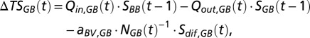where is the change in total amount of salt of the deep water in the Gotland Basin across years, is the salinity of the inflowing deep water from the previous year that is flushed into the Słupsk Furrow, and is the salinity in the Gotland Basin deep waters in the previous year. The last term describes the vertical mixing of salt across the halocline. Following Stigebrandt (38), it is assumed that the turbulent diffusion coefficient is inversely related to the Brunt–Väisälä frequency . The scaling parameter is denoted and the salinity difference across the halocline is .

The balance for AOU follows the same principle but with the addition of an oxygen consumption term.

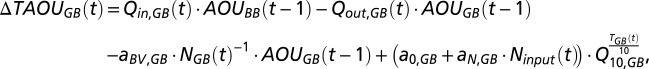where is the change in TAOU of the deep water in the Gotland Basin across years, and are the AOUs in the deep waters in the two basins of the previous year, and and are two parameters describing how oxygen consumption is linearly related to the input of either total nitrogen or total phosphorus , and scaled by temperature with a Q₁₀-parameter . Time series of nitrogen and phosphorus inputs (1850–2006) were taken from ref. 8. It is assumed that the surface water is saturated in oxygen (AUO = 0). The increasing AOU in the Bornholm Basin over time implies that the export of AOU to the Gotland Basin has increased. The unknown parameters in the water, salt, and oxygen balances above ( and ) were estimated by maximum-likelihood estimation from time series of total salinity and TAOU. Moving averages of 5 y were used for estimation to overcome small gaps in the time series, and because time differences [ and ] of the annual values introduced large noise in the equations and consequently, large uncertainty in the parameter estimates. Thus, the model was essentially estimated on three time series sequences: 1903–1910, 1922–1938, and 1954–2006, where all input time series were nonmissing.

Changes in the lateral flows and mixing across the halocline significantly affected TAOU, and to assess the TAOU trend without these physical modulations, the dynamic flow and mixing terms [, and ] were subtracted and replaced by average values for the study period. The difference between the TAOU and the adjusted TAOU was set to zero at the start of each of the three time series sequences.

References

- 1.Stramma L, Johnson GC, Sprintall J, Mohrholz V. Expanding oxygen-minimum zones in the tropical oceans. Science. 2008;320(5876):655–658. doi: 10.1126/science.1153847. [DOI] [PubMed] [Google Scholar]
- 2.Díaz RJ, Rosenberg R. Spreading dead zones and consequences for marine ecosystems. Science. 2008;321(5891):926–929. doi: 10.1126/science.1156401. [DOI] [PubMed] [Google Scholar]
- 3.Levitus S, et al. Global ocean heat content 1955–2008 in light of recently revealed instrumentation problems. Geophys Res Lett. 2009;36(7):L07608. [Google Scholar]
- 4.Rabalais NN, Turner RE, Wiseman WJ., Jr Gulf of Mexico hypoxia, A.K.A. “The Dead Zone”. Annu Rev Ecol Syst. 2002;33:235–263. [Google Scholar]
- 5.Kemp WM, Testa J, Conley DJ, Gilbert D, Hagy J. Temporal responses of coastal hypoxia to nutrient loading and physical controls. Biogeosciences. 2009;6(12):2985–3008. [Google Scholar]
- 6.Kabel K, et al. Impact of climate change on the Baltic Sea ecosystem over the past 1,000 years. Nat Clim Change. 2012;2(12):871–874. [Google Scholar]
- 7.Conley DJ, et al. Hypoxia-related processes in the Baltic Sea. Environ Sci Technol. 2009;43(10):3412–3420. doi: 10.1021/es802762a. [DOI] [PubMed] [Google Scholar]
- 8.Gustafsson BG, et al. Reconstructing the development of Baltic sea eutrophication 1850–2006. Ambio. 2012;41(6):534–548. doi: 10.1007/s13280-012-0318-x. [DOI] [PMC free article] [PubMed] [Google Scholar]
- 9.Stigebrandt A, Gustafsson BG. Response of the Baltic Sea to climate change—theory and observations. J Sea Res. 2003;49(4):243–256. [Google Scholar]
- 10.Döös K, Meier HEM, Döscher R. The Baltic haline conveyor belt or the overturning circulation and mixing in the Baltic. Ambio. 2004;33(4-5):261–266. [PubMed] [Google Scholar]
- 11.Gustafsson BG, Andersson HC. Modeling the exchange of the Baltic Sea from the meridional atmospheric pressure difference across the North Sea. J Geophys Res. 2001;106(C9):19731–19744. [Google Scholar]
- 12.Schinke H, Matthäus W. On the causes of major Baltic inflows—an analysis of long time series. Cont Shelf Res. 1998;18(1):67–97. [Google Scholar]
- 13.Meier HEM. Modeling the pathways and ages of inflowing salt- and freshwater in the Baltic Sea. Estuar Coast Shelf Sci. 2007;74(4):610–627. [Google Scholar]
- 14.Conley DJ, Humborg C, Rahm L, Savchuk OP, Wulff F. Hypoxia in the Baltic Sea and basin-scale changes in phosphorus biogeochemistry. Environ Sci Technol. 2002;36(24):5315–5320. doi: 10.1021/es025763w. [DOI] [PubMed] [Google Scholar]
- 15.Rabalais NN, Turner RE, Diaz RJ, Justic D. Global change and eutrophication of coastal waters. ICES J Mar Sci. 2009;66(7):1528–1537. [Google Scholar]
- 16.Fonselius S, Valderama J. One hundred years of hydrographic measurements in the Baltic Sea. J Sea Res. 2003;49(4):229–241. [Google Scholar]
- 17.Savchuk O, Wulff F, Hille S, Humborg C, Pollehne F. The Baltic Sea a century ago—a reconstruction from model simulations, verified by observations. J Mar Syst. 2008;74(1-2):485–494. [Google Scholar]
- 18.Nausch G, Nehring D, Nagel K. In: State and Evolution of the Baltic Sea, 1952–2005. Feistel R, Nausch G, Wasmund N, editors. Hoboken, NJ: Wiley; 2008. pp. 337–366. [Google Scholar]
- 19.Hagy JD, Boynton WR, Keefe CW, Wood KV. Hypoxia in Chesapeake Bay, 1950–2001: Long-term change in relation to nutrient loading and river flow. Estuaries. 2004;27(4):634–658. [Google Scholar]
- 20.Graham LP. Climate change effects on river flow to the Baltic Sea. Ambio. 2004;33(4-5):235–241. [PubMed] [Google Scholar]
- 21.Vahtera E, et al. Internal ecosystem feedbacks enhance nitrogen-fixing cyanobacteria blooms and complicate management in the Baltic Sea. Ambio. 2007;36(2-3):186–194. doi: 10.1579/0044-7447(2007)36[186:iefenc]2.0.co;2. [DOI] [PubMed] [Google Scholar]
- 22.Kritzberg ES, Ekström SM. Increasing iron concentrations in surface waters—a factor behind brownification? Biogeosciences. 2012;9(4):1465–1478. [Google Scholar]
- 23.Wikner J, Andersson A. Increased freshwater discharge shifts the trophic balance in the coastal zone of the northern Baltic Sea. Glob Change Biol. 2012;18(8):2509–2519. [Google Scholar]
- 24.Duarte CM, Conley DJ, Carstensen J, Sánchez-Camacho M. Return to Neverland: Shifting baselines affect eutrophication restoration targets. Estuaries Coasts. 2009;32(1):29–36. [Google Scholar]
- 25.Levin LA, et al. Effects of natural and human-induced hypoxia on coastal benthos. Biogeosciences. 2009;6(10):2063–2098. [Google Scholar]
- 26.Stramma L, et al. Expansion of oxygen minimum zones may reduce available habitat for tropical pelagic fishes. Nat Clim Change. 2012;2(1):33–37. [Google Scholar]
- 27.Karlson K, Rosenberg R, Bonsdorff E. Temporal and spatial large-scale effects of eutrophication and oxygen deficiency on benthic fauna in Scandinavian and Baltic waters—a review. Oceanogr Mar Biol. 2002;40:427–489. [Google Scholar]
- 28.Villnäs A, Norkko A. Benthic diversity gradients and shifting baselines: Implications for assessing environmental status. Ecol Appl. 2011;21(6):2172–2186. doi: 10.1890/10-1473.1. [DOI] [PubMed] [Google Scholar]
- 29.Elmgren R. Man's impact on the ecosystem of the Baltic Sea: Energy flows today and at the turn of the century. Ambio. 1989;18(6):326–332. [Google Scholar]
- 30.MacKenzie BR, Hinrichsen H-H, Plikshs M, Wieland K, Zezera AS. Quantifying environmental heterogeneity: Habitat size necessary for successful development of cod Gadus morhua eggs in the Baltic Sea. Mar Ecol Prog Ser. 2000;193:143–156. [Google Scholar]
- 31.Conley DJ, Carstensen J, Vaquer-Sunyer R, Duarte CM. Ecosystem thresholds with hypoxia. Hydrobiologia. 2009;629:21–29. [Google Scholar]
- 32.Funkey CP, et al. 2014. Hypoxia sustains cyanobacteria blooms in the Baltic Sea. Environ Sci Technol 48(5):2598–2602.
- 33.Conley DJ. Ecology: Save the Baltic Sea. Nature. 2012;486(7404):463–464. doi: 10.1038/486463a. [DOI] [PubMed] [Google Scholar]
- 34.Helsinki Commission for Protection of the Baltic Sea 2007. HELCOM Baltic Sea Action Plan. Available at www.helcom.fi/Documents/Baltic%20sea%20action%20plan/BSAP_Final.pdf. Accessed March 21, 2014.
- 35.Gustafsson B. Time-dependent modeling of the Baltic entrance area. 1. Quantification of circulation and residence times in the Kattegat and the Straits of the Baltic Sill. Estuaries. 2000;23(2):231–252. [Google Scholar]
- 36.Conley DJ, et al. Hypoxia is increasing in the coastal zone of the Baltic Sea. Environ Sci Technol. 2011;45(16):6777–6783. doi: 10.1021/es201212r. [DOI] [PMC free article] [PubMed] [Google Scholar]
- 37.Lass HU, Matthäus W. In: State and Evolution of the Baltic Sea, 1952–2005. Feistel R, Nausch G, Wasmund N, editors. Hoboken, NJ: Wiley; 2008. pp. 5–43. [Google Scholar]
- 38.Stigebrandt A. Computations of the flow of dense water into the Baltic Sea from hydrographical measurements in the Arkona Basin. Tellus. 1987;39A(2):170–177. [Google Scholar]
- 39.Carstensen J. Censored data regression: Statistical methods for analyzing Secchi transparency in shallow systems. Limnol Oceanogr Methods. 2010;8:376–385. [Google Scholar]
Associated Data
This section collects any data citations, data availability statements, or supplementary materials included in this article.