

Abstract
A Bayesian alignment model (BAM) is proposed for alignment of liquid chromatography-mass spectrometry (LC-MS) data. BAM belongs to the category of profile-based approaches, which are composed of two major components: a prototype function and a set of mapping functions. Appropriate estimation of these functions is crucial for good alignment results. BAM uses Markov chain Monte Carlo (MCMC) methods to draw inference on the model parameters and improves on existing MCMC-based alignment methods through 1) the implementation of an efficient MCMC sampler and 2) an adaptive selection of knots. A block Metropolis-Hastings algorithm that mitigates the problem of the MCMC sampler getting stuck at local modes of the posterior distribution is used for the update of the mapping function coefficients. In addition, a stochastic search variable selection (SSVS) methodology is used to determine the number and positions of knots. We applied BAM to a simulated data set, an LC-MS proteomic data set, and two LC-MS metabolomic data sets, and compared its performance with the Bayesian hierarchical curve registration (BHCR) model, the dynamic time-warping (DTW) model, and the continuous profile model (CPM). The advantage of applying appropriate profile-based retention time correction prior to performing a feature-based approach is also demonstrated through the metabolomic data sets.
Keywords: Alignment, Bayesian inference, block Metropolis-Hastings algorithm, liquid chromatography-mass spectrometry (LC-MS), Markov chain Monte Carlo (MCMC), stochastic search variable selection (SSVS)
1 Introduction
Recent advances in liquid chromatography-mass spectrometry (LC-MS) technology have led to more effective approaches for measuring expression levels of biomolecules in various “-omics” studies including proteomics, metabolomics, and glycomics [1], [2], [3]. Each LC-MS run generates data consisting of thousands of ion intensities characterized by their specific retention time (RT) and mass-to-charge ratio (m/z) values. Label-free LC-MS methods [4], [5] have been used for extraction of quantitative information and for detection of differentially abundant features. However, difference detection using label-free LC-MS methods requires that various preprocessing steps including peak detection, RT alignment, peak matching, normalization, and missing value imputation be appropriately handled [6]. Typically, these preprocessing steps generate a list consisting of detected peaks with their RT and m/z values and the intensities from multiple LC-MS runs, followed by statistical tests to identify significant differences. A crucial step is to correctly match unique peaks across multiple LC-MS runs. Highly precise and accurate mass measurement has become achievable with the continuous improvement of MS technology [7]. The LC processes, however, are less reproducible and usually result in substantial variation in RT across multiple LC-MS runs [8], raising significant challenges in the preprocessing pipeline. Without appropriate correction, the subsequent analysis may yield misleading results.
Alignment approaches can be roughly classified into two categories [8]: 1) feature-based approaches and 2) profile-based approaches. The feature-based approaches [9], [10], [11], [12] proceed with the alignment of the detected features (usually referred to as peaks) directly. Consensus peaks across multiple runs are first identified based on some predefined tolerance ranges. With this matching information, RT correction can then be carried out seamlessly. Identification of the consensus peaks is key to the success of the feature-based approaches. The results are highly dependent on the peaks detected upfront. Moreover, since peak detection is carried out for each LC-MS run separately, methods that do not leverage information from multiple LC-MS runs have the additional challenge of dealing with missing data and identifying consensus peaks correctly. The profile-based approaches [13], [14], on the other hand, make use of chromatograms of the LC-MS runs to estimate the variability along RT and adjust the LC-MS runs accordingly. It is assumed that there exists a pattern underlying multiple chromatograms from the same biological group and that the profile variability is relatively small compared to distortions caused by misalignment. Compared to a set of RT points utilized by the feature-based approaches, the chromatograms provide more comprehensive information about the variation throughout the whole RT range. This could benefit the alignment task if the RT variation is estimated effectively and correctly, which is the main focus of this paper. In addition to the formulation of alignment problem and required input data, these two types of alignment approaches differ in the coverage of the pre-processing pipeline. The profile-based approaches address the problem of alignment, while the feature-based approaches deal simultaneously with the alignment and peak matching. We propose to first adjust the RT values based on the alignment result then subsequently address the peak matching as described in Section 3.3.
Fig. 1 presents the concept of a profile-based approach. The algorithm searches for 1) a prototype function that characterizes the consistent pattern across samples and 2) a set of mapping functions that characterize the relationship between the prototype function and the observed data. The goal is to estimate the underlying prototype/mapping functions most likely to have generated the observed data. The main challenge in profile-based approaches, such as dynamic time warping (DTW) and correlation optimized warping (COW) [13], is related to the choice of a prototype function, which is unknown and needs to be estimated by considering all the observations in the data. Most of the existing alignment approaches are based on hard selection of a reference (profile or feature), which does not allow any adjustment of the reference during alignment. Considering the lack of consistent pattern across samples relative to the fixed reference, important information may be missed. To address this concern, some generative models were proposed to estimate the reference from the observations. One of the most effective models is called continuous profile model (CPM) [14]. CPM is developed in a probabilistic framework and both prototype and mapping functions are simultaneously estimated from the observations. However, the strategy of mapping the data onto a higher-dimensional space may limit its applicability to high-resolution LC-MS data.
Fig. 1.
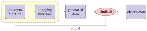
Profile-based approach is composed of two components: prototype function and mapping functions, which are estimated from the observed data and are used to align the chromatograms in the proposed BAM.
Another issue of the current alignment approaches (both feature based and profile based) is the lack of uncertainty assessment. A measure of uncertainty is desired to provide a confidence level in the alignment results and assist in making decisions for subsequent analyses or data integration. In spike-in experiments or studies utilizing MS/MS identification results, the integration of this complementary information has been found to lead to better alignment results, for example, in [15], [16]. However, the integration is often implemented through ad hoc approaches, partly due to the lack of uncertainty measures. In combining the information from various sources, accounting for the uncertainty in the alignment from each source may lead to improved results.
In this paper, we present a profile-based Bayesian alignment model (BAM) for LC-MS data. To our knowledge, there is currently no method that addresses the uncertainty issue for LC-MS data alignment. Relevant work in other application areas include the hierarchical Bayesian continuous profile model (HB-CPM), which was proposed and applied to liquid chromatography-ultraviolet (LC-UV) data analysis [17], and a Bayesian hierarchical model for curve registration (BHCR) [18], which uses a Markov chain Monte Carlo (MCMC) method for parameter inference. For alignment of LC-MS data, which consist of many chromatographic peaks, more flexible MCMC algorithms are desired. We observe that the element-wise Metropolis-Hastings algorithm utilized in BHCR is prone to overfitting due to inefficient MCMC moves. To overcome this problem, we propose a block Metropolis-Hastings algorithm using a mixture of block transition moves [19] for more flexible and effective updates. In addition, a stochastic search technique is built into BAM to enable adaptive knot specification for the mapping functions. For LC-MS data where chromatographic peaks are not homogeneously present along RT, a uniformly distributed knot specification is not desirable. Instead of fixing the knots upfront, we propose using stochastic search variable selection (SSVS) [20] to determine the number and positions of knots. For performance evaluation, we applied BAM to a simulated data set, an LC-MS proteomic data set, and two LC-MS metabolomic data sets. We compared BAM with other profile-based alignment approaches using correlation coefficients and ratio of peak distortion. The advantage of applying BAM for RT correction prior to performing a feature-based approach is also demonstrated through the metabolomic data sets.
The remainder of this paper is organized as follows: Section 2 introduces the methodology of the proposed BAM. The hierarchical model, the block Metropolis-Hastings algorithm, the posterior inference for the model parameters, and the SSVS procedure for knot specification are described in this section. Section 3 demonstrates applications of BAM to both simulated and real LC-MS data sets, and compares its performance to various methods. Finally, Section 4 concludes the paper with a summary and possible extensions for future work.
2 Model Formulation
A BAM is proposed for LC-MS data alignment. We address the alignment problem within a Bayesian framework. The inference for the model parameters is based on their posterior distributions, which are estimated using MCMC methods.
2.1 Bayesian Alignment Model
BAM is a generative model that performs RT alignment based on multiple chromatograms of LC-MS runs. The chromatograms are obtained based on total ion count or base peak intensity. In some applications, a screening step is helpful to filter out baselines or noises in certain m/z values. The observed chromatograms from N replicates, yi(t), i = 1, … N, t = t1, … tT, are assumed to share a similar profile characterized by the prototype function m(t). We use a piecewise linear function to model the nonlinear variability [11] along RT. For the ith chromatogram at RT t, the intensity value is referred to as the prototype function indexed by the mapping function ui(t), i.e.,m(ui(t)). Fig. 2 illustrates the relationship between the sample and the prototype function through the mapping function. The intensity of the sample at time 1, for example, is referred to as the intensity of the prototype function at time ui(1) = 2, that is m(2) = 3.
Fig. 2.

An illustrative example showing the functionalities of the prototype function m(t) and the mapping function ui(t). For example, the intensity of the sample at time t = 1 corresponds to the intensity of the prototype function at time ui(1) = 2, which is given by m(2) = 3.
By incorporating the variability of intensity using affine transformation, each chromatogram is modeled as
| (1) |
where ai and ci are scaling and translation parameters, and the errors ∊i(t) are independent and identically distributed normal random variables . These parameters characterize the individual variability of each chromatogram. Conjugate normal prior distributions are chosen for ai and ci, i.e., and .
The prototype function is modeled with B-spline regression:
| (2) |
where , , and . The regression coefficients for the prototype function, ψ, are specified by a first-order random walk: , where ψ0 = 0.
The mapping function ui(t) is a piecewise linear function characterized by a set of knots τ = (τ0, τ1 … ,τK+1) and their corresponding mapping indices φi = (φi,0, φi,1, … , φi, K+1), where τ0 = t1 and τK+1 = tT. The mapping function is defined in terms of τ and φ:
| (3) |
To keep the elution order of LC process, the monotonicity constraint φi,0 < ⋯ < φi,K+1 needs to be satisfied. The prior of φi is specified via a slope value ωi = (ωi,1, … , ωi,K+1)⊺, where ωi,j assumed to follow a normal distribution with mean ωi,j−1 and variance truncated below by 0 to ensure monotonicity of φi, and is defined as ωi,j = (φi,j − φi, j−1)/(τ − τj−1. The prior of φi is, therefore, given by
| (4) |
where ωi, 0 and pTN(·) corresponds to the truncated normal density function. Finally, we specify the priors for the other model parameters to complete the hierarchy:
These priors are chosen to be conjugate to the likelihood function. Fig. 3 presents the directed acyclic graph of BAM, where the model parameters are represented by open circles, the hyperparameters by solid dots, and the observations by filled circles.
Fig. 3.

Directed acyclic graph of BAM.
2.2 Posterior Inference
Based on the generative model introduced in Section 2.1, the alignment problem is translated into an inference task: given the chromatograms y = {y1, y2, … , yN}, we need to estimate the model parameters {a, c, ψ, φ, a0, c0, , , , }. Once the inference is complete, the alignment can be carried out by applying an inverse mapping function to each chromatogram, i.e., . The parameter inference is drawn using MCMC methods. For the parameters whose full conditionals have closed forms, θ = {a, c, ψ, a0, c0, , , , }, we use the Gibbs sampler to update their values (please refer to Appendix A, available in the online supplemental material, which can be found on the Computer Society Digital Library at http://doi.ieeecomputersociety.org/10.1109/TCBB.2013.25, for the full conditionals of these parameters.) The remaining parameters, i.e., the mapping function coefficients, φ = {φ1, … , φN}, are updated using a Metropolis-Hastings algorithm with a uniform proposal density that reflects the constraints on the boundaries.
Algorithm 1 outlines one iteration of the MCMC procedure. The transition ratio rT for the proposal density is one, while the likelihood ratio rL and prior ratio rP in the Metropolis-Hastings acceptance probability, rA, for updating are given by
| (5) |
| (6) |
where denotes the set of coefficients φi at iteration m + 1 with φi,j excluded, i.e., . The MCMC move for updating φi,j changes the slopes ωi,j and ωi,j+1, and consequently the involved densities.
Algorithm 1. MCMC update of (θ(m, φ(m)
for all φi,j do
end for
2.3 Block Metropolis-Hastings Algorithm
When the misalignment involves translation shift along RT, the element-wise Metropolis-Hastings move for φi requires a series of successive proposals in the same direction to be accepted sequentially. This incremental update hinders the mixing of the MCMC sampler. In addition, the monotonicity constraint inhibits the flexibility of the proposal to consider relatively large changes for each of the mapping function coefficients. To address this issue, we consider block proposal moves [19] to allow a set of successive coefficients to be adjusted simultaneously. Rather than updating each coefficient φi,j sequentially, the φi,js are first grouped into several nonoverlapping blocks, which consist of successive coefficients along the RT, and proposals are made to update each block. The block move offers a more efficient way to update the coefficients, which improves the mixing of the MCMC sampler.
We introduce binary indicator variables bj, ∈ {0, 1}, j = 1, … , K, to identify the block boundaries, where bj = 1 if τj is at the boundary of a block and b0 = bK+1 = 1. This indicator variable follows a Bernoulli distribution with p(bj = 1) = rblock. Based on the boundary configuration, coefficients within the same block φi,j:j+Bj−1 = (φi,j, φi,j+1, … φi,j+Bj−1), are proposed to be moved in the same direction, where bj = bj+Bj = 1 and bj+1 = ⋯ = bj+Bj1− = 0. The element-wise move can be viewed as a special case of the block move where rblock = 1 and each block only contains a single coefficient. We consider a mixture of transitions where rblock is randomly selected from {1, 1/2, 1/4, 1/8} at each iteration. The configuration of blocks is, therefore, variable within a Markov chain. We summarize the procedure for the block Metropolis-Hastings technique in Algorithm 2.
Algorithm 2. Block Metropolis-Hastings algorithm
for all block φi,j+Bj−1 do
end for
2.4 Number and Positions of Knots
Knot specification for the mapping functions is crucial to the alignment result. Although accurate alignment requires sufficiently dense knots to enable precise adjustments, an overly dense knot specification restricts the transition flexibility and is prone to overfitting. We address the knot specification issue using SSVS. At each iteration, along with the update of all model parameters (θ, φ), a change is proposed for the knot specification using one of the following transition moves: 1) knot inclusion—adding a knot into the current knot list, and 2) knot exclusion—removing a knot from the current knot list. In BAM, the first and the last time points are set as fixed knots, i.e., unchanged throughout the Markov chain, to control the span range of mapping function. For the middle T − 2 time points, t2, … tT−1, K of them are determined as knots and their placement is (τ1, … τK). A binary indicator variable associated with each time point γt is introduced to denote if a knot is present at time t, that is, γt = 1 if t belongs to (τ1, … , τK) and γt = 0 otherwise. This binary indicator is assumed to follow a Bernoulli distribution with p(γt = 1) = rknot, and thus, the probability density of a valid knot specification is given by
| (7) |
We estimate the knot specification for each chromatogram separately, i.e., each mapping function ui is defined by its own set of knots τi and mapping function coefficients φi. To keep the following discussion uncluttered, we make a slight abuse of notation by dropping the index of chromatogram i. At each iteration, after the update of (θ, φ), one of the middle T − 2 time points is randomly sampled from a uniform distribution, i.e., , and its corresponding γt is proposed to be updated to such that . The procedure for each proposal is summarized as follows:
- Knot inclusion
-
-When γt = 0 and τk−1 < t < τk, add t into the knot list (), such that the new set of knots becomes .
-
-Sample the mapping function coefficient for the new knot from a normal distribution truncated below by φk−1 and above by φk, , such that the new set of mapping function coefficients becomes , where μ = φk−1 · (τk−t)/(τk−τk−1) + φk · (t - τk−1)/(τk−τk−1) and σ = min{φk − μ, μ − φk−1}/4.
-
-Calculate the acceptance probability for (γ, τ, φ → γ′, τ′, φ′).
-
-
- Knot exclusion
-
-When γt = 1 and t = τk, remove t from the knot list (), such that the new set of knots and the mapping function coefficients become and
-
-Calculate the acceptance probability for (γ, τ, φ → γ′, τ′, φ′)
-
-
The probability for accepting a proposed move involves the likelihood ratio, the prior ratio, and the transition ratio. Details of the acceptance probability calculation are provided in Appendix B, available in the online supplemental material.
3 Results and Discussion
We applied BAM to a simulated data set, an LC-MS proteomic data set and two LC-MS metabolomic data sets. The performance of BAM was compared with that of the BHCR model [18], the DTW model [13], and the CPM [14]. The advantage of applying appropriate RT correction prior to performing a feature-based approach is demonstrated through the LC-MS metabolomic data sets.
3.1 Simulated Data Set
We generated a profile pattern composed of three Gaussian peaks with the same standard deviation but distinct mean values:
where μ1 = 10, μ2 = 15, μ3 = 40 σ = 1.25, and t = 1, … , 50. The mapping function ui was generated through the even-numbered order statistics as described in [21] to model the RT variability. Ten replicate runs were generated by the formulation:
where no RT variation was applied to the first replicate run, i.e., u1(t) = t. Random noises were produced based on signal-to-noise ratio (SNR). Three values of SNR (20, 25, and 30 dB) were considered. Fig. 4 depicts one realization of the simulated data with different noise levels, where the first replicate run is highlighted in bold. The data set simulates the scenario where location of peaks is not uniformly distributed along the time range, and different choices of knot specification may lead to distinct results.
Fig. 4.

One realization of simulated data with different noise levels: (a) no noise, (b) SNR 30, (c) SNR 25, and (d) SNR 20. The first replicate run with no time variation applied is highlighted in bold.
The first replicate run is used as reference for assessing alignment performance based on two measurements: 1) correlation coefficient, and 2) ratio of peak distortion. To assess the variability among replicate runs, we calculated the mean of the correlation coefficients between the first replicate run, generated with no RT variability, and the remaining nine replicate runs. It should be emphasized that the correlation coefficients can exaggerate the true alignment performance as the values do not reflect potential losses of chromatographic information. Thus, to ensure the peak patterns are not significantly distorted during alignment, we calculated the ratio of peak distortion defined as
to reflect the degree of peak preservation between the alignment using the estimated mapping functions versus the alignment using the true mapping functions.
We compare the performance of four alignment methods on the simulated data set: DTW, CPM, BHCR, and BAM (with fixed knots and with SSVS). Three values of knot density (0.1, 0.2, and 0.5) with equally spaced knots are considered for BHCR and BAM with fixed knots. The fixed knot specification for BAM is mainly for comparison purpose. In addition, BAM with SSVS, which automatically handles the knot specification, is applied to the data. Table 1 summarizes the performance measurements before alignment and after alignment using each of the four methods. The results for the simulated data are based on 500 realizations.
TABLE 1.
Correlation Coefficients and Ratio of Peak Distortion for the Simulated LC-MS Data, before Alignment (Original) and after Alignment by DTW, CPM, BHCR, and BAM (with Fixed Knots and with SSVS)
| SNR | Original | DTW | CPM | BHCR |
BAM |
||||||
|---|---|---|---|---|---|---|---|---|---|---|---|
| 0.1 | 0.2 | 0.5 | 0.1 | 0.2 | 0.5 | SSVS | |||||
| ∞ | 0.639 (0.060) |
0.918 (0.030) |
0.964 (0.017) |
0.938 (0.016) |
0.960 (0.016) |
0.735 (0.079) |
0.937 (0.016) |
0.962 (0.013) |
0.955 (0.031) |
0.970 (0.010) |
Correlation coeff. |
|
| |||||||||||
| 30 | 0.596 (0.060) |
0.880 (0.034) |
0.936 (0.019) |
0.893 (0.021) |
0.907 (0.022) |
0.685 (0.073) |
0.892 (0.021) |
0.911 (0.017) |
0.894 (0.038) |
0.916 (0.016) |
|
|
| |||||||||||
| 25 | 0.520 (0.060) |
0.823 (0.038) |
0.882 (0.021) |
0.806 (0.031) |
0.812 (0.034) |
0.602 (0.068) |
0.805 (0.032) |
0.819 (0.030) |
0.781 (0.057) |
0.821 (0.028) |
|
|
| |||||||||||
| 20 | 0.379 (0.055) |
0.710 (0.053) |
0.760 (0.040) |
0.616 (0.051) |
0.612 (0.057) |
0.465 (0.065) |
0.616 (0.052) |
0.627 (0.050) |
0.565 (0.064) |
0.629 (0.052) |
|
|
| |||||||||||
| ∞ | 0.168 (0.041) |
0.091 (0.047) |
0.064 (0.029) |
0.079 (0.020) |
0.063 (0.019) |
0.142 (0.042) |
0.079 (0.020) |
0.062 (0.018) |
0.064 (0.024) |
0.054 (0.016) |
Peak distortion |
|
| |||||||||||
| 30 | 0.170 (0.044) |
0.099 (0.050) |
0.072 (0.031) |
0.083 (0.021) |
0.075 (0.022) |
0.147 (0.047) |
0.083 (0.021) |
0.074 (0.021) |
0.081 (0.026) |
0.070 (0.020) |
|
|
| |||||||||||
| 25 | 0.175 (0.044) |
0.106 (0.043) |
0.082 (0.029) |
0.091 (0.024) |
0.089 (0.025) |
0.159 (0.045) |
0.091 (0.024) |
0.088 (0.025) |
0.099 (0.034) |
0.086 (0.022) |
|
|
| |||||||||||
| 20 | 0.175 (0.042) |
0.135 (0.051) |
0.105 (0.033) |
0.102 (0.027) |
0.110 (0.032) |
0.170 (0.044) |
0.101 (0.026) |
0.099 (0.027) |
0.128 (0.036) |
0.100 (0.027) |
|
Means (standard deviations) are reported for the simulated data based on 500 realizations.
In terms of correlation coefficient and ratio of peak distortion, significant improvements are observed after alignment by all the methods. DTW yields good performance in terms of correlation coefficient. However, the result based on ratio of peak distortion suggests that the profiles are overly distorted in the effort to make them resemble each other. This phenomenon is undesirable because meaningful information is lost during the alignment. CPM and BAM with SSVS are the two leading models. CPM adjusts both time and intensity and yields the best correlation coefficient values except for the case with no noise added. On the other hand, BAM with SSVS outperforms other models in terms of ratio of peak distortion. It also yields higher correlation coefficients in the case with no noise. This indicates the peak patterns are better restored and alignment toward noises is not favored by BAM. The difference between BAM with fixed knots and BHCR is due to the ability of BAM to overcome the mixing problem of standard MCMC methods in multimodal models by using block Metropolis-Hastings updates, whereas BHCR is prone to getting stuck at local modes by relying on incremental updates. The distinction becomes significant with knot density of 0.5, where BHCR leads to the worst performance in terms of both measurements. As discussed in Section 2.4, accurate alignment requires sufficiently dense knot placement while naïvely increasing the number of knots may lead to overfitting. This is primarily due to monotonicity constraint for the parameter φ being controlled by the positions of the knots. Selecting a good knot specification setting is even more involved in practical applications because there is no ground truth available on which to calibrate. This problem is circumvented by the adaptive selection of knots in BAM with SSVS, which provides an automatic approach to place knots adaptively, according to the complexity of the underlying profile.
3.2 LC-MS Proteomic Data Set
The spike-in data set by Listgarten et al. [22] consists of two aliquots of the same human serum sample, where the second aliquot has three known peptides spiked in. Seven replicate LC-MS runs from each aliquot were acquired using a capillary-scale LC coupled to an ion trap mass spectrometer. Each run is preprocessed and represented by a 501 (RT points) × 2,401 (m/z bins) data matrix. To know the true differences between the two aliquots in the LC-MS data, eight ground-truth runs from a mixture of spiked-in peptides (without serum) were acquired and 32 experimentally detected m/z values of ground truth were reported. The spike-in experiment can help to evaluate alignment results based on the true differences spiked in the sample. Detailed experimental information can be found in [22].
Fig. 5 depicts the base peak chromatograms of the 14 LC-MS runs, where significant shifts are observed along the RT points. We applied four models, DTW, CPM, BHCR, and BAM to align the chromatograms (Fig. 6). The alignment result by DTW is shown in Fig. 6a. Similar to our observation in Section 3.1, DTW is prone to overly distorting the profiles and the estimator often gets stuck in local optima. CPM yields the best performance in this data set in terms of both visual assessment (Fig. 6b) and correlation coefficients as shown in Table 2. In general, it works quite well on problems with moderate dimension (less than 1,000). The results by the two Bayesian models, BHCR and BAM are shown in Figs. 6c and 6d, respectively. In the result by BHCR, several peaks from two replicates of the second aliquot are not correctly aligned to the majority of peaks in RT range 100-250. Instead, they are mistakenly aligned to other tiny peaks around their original RTs. A similar issue is observed in the DTW result. As mentioned in Section 2.3, the element-wise Metropolis-Hastings move utilized in BHCR is prone to getting stuck at local modes. It is particularly hard to get away from the trap if the true parameter values are far from the current values and lie beyond the range of values that can be proposed by the Markov chain transition moves. In contrast to BHCR, this trapping effect is overcome by BAM as shown in Fig. 6d. The inference was based on 15,000 MCMC iterations obtained after discarding the initial 5,000 iterations as burn-in. The knot specification is automatically handled with the SSVS procedure. Fig. 7a shows the trace plot of the number of knots selected at each MCMC iteration for the chromatogram from the seventh replicate of the second serum aliquot; we see that it stabilizes around 60 knots. Fig. 7b gives a summary of the numbers of knots across the models visited by the MCMC sampler for each of the 14 chromatograms based on 15,000 MCMC iterations obtained after discarding the initial 5,000 iterations.
Fig. 5.

(a) Base peak chromatograms of the original LC-MS data. (b) Zooms in the RT range 100-250 for the chromatograms in (a).
Fig. 6.

Aligned chromatograms by (a) DTW, (b) CPM, (c) BHCR, and (d) BAM. (e), (f), (g), and (h) zoom in the RT range 100-250 for the chromatograms in (a), (b), (c), and (d), respectively. Misalignments by DTW and BHCR are observed in (e) and (g).
TABLE 2.
Correlation Coefficients for the LC-MS Proteomic Data, before Alignment (Original) and after Alignment by DTW, CPM, BHCR (with Knot Density of 0.2), and BAM (with SSVS)
| Original | DTW | CPM | BHCR | BAM | |
|---|---|---|---|---|---|
| Aliquot 1 | 0.35 | 0.86 | 0.95 | 0.92 | 0.92 |
| Aliquot 2 | 0.28 | 0.88 | 0.94 | 0.77 | 0.91 |
Fig. 7.

(a) Trace plot of the number of knots in the models visited at each MCMC iteration for the chromatogram from the seventh replicate of the second serum aliquot. (b) Box plot of the number of knots visited by the MCMC sampler for each chromatogram.
Finally, according to the ground truth of 32 m/z values reported in [22], we observe a clear contrast in the extracted ion chromatograms (EICs) of 16 m/z values (433.63, 513.50, 524.48, 535.00, 601.03, 615.60, 647.50, 649.11, 674.93, 699.03, 784.50, 811.00, 1,047.12, 1,297.43, 1,348.65, and 1,575.09) between two sets of LC-MS runs corresponding to the “presence” and “absence” of spiked-in peptides. We use these EICs to demonstrate the alignment performance. For the other 16 m/z values, we have been unable to observe the differences in their EICs. Fig. 8 depicts EICs before and after alignment by BAM for m/z values 1,047.12 and 1,575.09 in the absence and presence of spiked-in peptides. The figure demonstrates that the RT shifts observed in the EICs are effectively corrected by applying BAM. In addition, compared to the EICs prior to the alignment, the aligned EICs exhibit more distinct and specific differences between the two sets of LC-MS runs in terms of the spiked-in peptides. Similar results were obtained for all the 16 m/z values by using BAM and CPM, which can be found in the supplementary material, available online.
Fig. 8.

EICs for selected m/z values of 1,047.12 and 1,575.09. For each m/z value, four plots showing the chromatograms of all seven replicates are depicted: chromatograms for aliquots with serum alone (left) and serum with spiked-in peptides (right) are shown before alignment (top) and after alignment by BAM (bottom).
3.3 LC-MS Metabolomic Data Set
Lange et al. [23] compared a set of feature-based alignment models on four publicly available data sets (two proteomic and two metabolomic data sets). In this benchmark study, peak detection was performed on the raw data and the resulting peak list was stored in a .featureXML file (format of OpenMS [24]) for each LC-MS run. In addition to the peak lists, the two metabolomic data sets, designated as M1 and M2 have raw data available in .mzData and .netCDF formats, respectively. To evaluate the alignment result, ground-truth data were generated based on ion annotation [25], correlation of chromatographic profile, and consistency of peak. Comparison was carried out by measuring recall and precision by the alignment models against the ground-truth data. For the details, we refer interested readers to the paper [23].
As discussed in Section 1, correct identification of the consensus peaks is crucial for the feature-based approaches. We presume that appropriate RT correction can facilitate this process and subsequently lead to improved performance. To confirm this idea, we applied DTW, CPM, and BAM to both M1 and M2 data sets based on the chromatograms extracted from the raw data, where M1 and M2 consist of 44 and 24 LC-MS runs, respectively. According to the estimated mapping functions, we modified the RT values in the peak lists, i.e., replace t by ui(t), and applied a feature-based alignment model, OpenMS [24] on the adjusted lists using the same m/z tolerances as in [23].
For each LC-MS run, binning along the m/z dimension was performed to obtain 100 binned chromatograms of identical total ion counts. Chromatogram quality was evaluated using the mass chromatographic quality (MCQ) value accounting for potential baseline and noise [26]. Those chromatograms with MCQ value less than 0.85 were screened out and the sums of the remaining ones were used as input to the profile-based models. Fig. 9 depicts the chromatograms in data sets M1 and M2, before and after alignment by BAM. By adjusting the RT values based on the BAM alignment result, the identification of the consensus peaks using the feature-based models is reduced to a simpler task. Table 3 presents the performance measurements, in terms of recall, precision, and F-measure, when using the feature-based model alone (uncoupled) and when coupling the profile-based models (DTW, CPM, and BAM) to the feature-based model. We note that applying first a profile-based alignment model can lead to improved results, although this is not always the case. If the mapping functions are not correctly estimated, this procedure can deteriorate the result by making the generation of consensus peaks even more difficult. Using DTW for RT correction yields improved performance on M2 but lower recall on M1. This may be due to the low SNR in the latter. We calculate the SNR for these data as
based on the posterior distribution estimated by BAM. The estimates of SNR are 18.58 and 41.07 in M1 and M2, respectively. The higher SNR in M2 suggests that better profiles are available for mapping function estimation and more accurate estimation result is expected. On the other hand, it is more challenging to align the noisy chromatograms in M1. As also demonstrated in Sections 3.1 and 3.2, DTW is prone to overfitting the data, which may overly distort the profile and fail to estimate the correct mapping function. The other considered profile-based model, CPM showed good performance in the simulated data and the LC-MS proteomic data. Unfortunately, we have been unable to effectively use CPM for RT correction in the metabolomic data sets, primarily due to the higher dimensional data (1,525 and 2,397 RT points in M1 and M2, respectively). The current version of CPM does not correctly estimate the mapping functions in M1 and fails to process the data in M2 due to numerical problems.1 As CPM maps the data onto a higher-dimensional space, efforts are needed for an attempt to apply the model to high-resolution LC-MS data. We note that using BAM for RT correction prior to performing the feature-based model leads to improved performance on both data sets, M1 and M2.
Fig. 9.

Chromatograms in the metabolomic data sets, M1 and M2, before and after alignment by BAM. The inset is a zoomed part in the middle RT range of the chromatograms.
TABLE 3.
Comparison of the Peak Matching Results by Using OpenMS Alone (Upcoupled) and Using Three Profile-Based Alignment Models for RT Correction Prior to Applying OpenMS (DTW+, CPM+ and BAM+) on the Metabolomic Data Sets
| OpenMS |
|||||
|---|---|---|---|---|---|
| Uncoupled | DTW+ | CPM+ | BAM+ | ||
| M1 | Recall | 0.87 | 0.85 | 0.34 | 0.88 |
| Precision | 0.69 | 0.74 | 0.68 | 0.74 | |
| F-measure | 0.77 | 0.79 | 0.45 | 0.80 | |
|
| |||||
| M2 | Recall | 0.93 | 0.97 | − | 0.97 |
| Precision | 0.79 | 0.83 | − | 0.83 | |
| F-measure | 0.85 | 0.89 | − | 0.89 | |
4 Conclusion
In this paper, we propose a BAM for LC-MS data analysis and use MCMC methods for parameter inference. BAM improves on existing Bayesian methods by 1) using an efficient MCMC sampler and 2) adaptively selecting knots for the mapping function. Due to the mathematical intractability of the mapping function and the monotonicity constraint imposed on it, designing an effective updating scheme is crucial to ensure good mixing of the MCMC sampler. We propose a block Metropolis-Hastings algorithm that enables flexible transition and prevents the sampler from getting trapped in local modes of the posterior distribution. Moreover, an extension using SSVS is provided for adaptive knot specification. For the profile-based alignment, evaluation on both simulated and real data sets shows improved alignment results in terms of correlation coefficients between chromatograms, ratio of peak distortion, as well as visual assessment relative to the ground truth. In addition, alignment by BAM is demonstrated to facilitate the subsequent peak matching process using two metabolomic benchmark data sets.
In general, effective proposals to correct significant misalignments are particularly desired at the beginning of Markov chains. Otherwise, the Markov chain might get stuck at a local mode and it would be difficult to make significant changes thereafter. Inefficient mixing in some range of the Markov chain may arise from the choice of the proposal distribution or the choice of tuning parameters. The current model gets around this problem through a mixture of transition densities. We are investigating adaptive ways for online evaluation and adjustment of the Metropolis-Hastings transition densities.
In addition to the considerations related to the MCMC implementation, various aspects of BAM deserve further investigation. For example, the current setting of BAM is based on a single chromatogram for each LC-MS run. Identifying representative EICs can potentially improve the alignment accuracy by providing more comprehensive information about the variability in RT across LC-MS runs. The strategy is computationally feasible because BAM can be extended to handle multiple chromatograms by introducing associated prototype functions accordingly. An important practical issue is how to extract informative EICs from an LC-MS run. Rather than naïvely binning along the m/z dimension, we are interested in utilizing informative metrics, such as MCQ value to select chromatograms, and effective clustering scheme to make the problem more manageable.
The main assumption of the profile-based alignment models is that a consistent pattern is representative of LC-MS runs for samples in the same biological group. When samples arise from different biological subgroups, the models need to be extended to account for the heterogeneity across these subgroups. A unified approach that allows the simultaneous alignment of samples from multiple groups will ensure coherence in the processing step and data comparability, which will facilitate downstream analyses, such as difference detection.
Supplementary Material
ACKNOWLEDGMENTS
This work was supported by the National Cancer Institute Grants R01CA143420 and U01CA160036.
Biography

Tsung-Heng Tsai is currently working toward the PhD degree in the Department of Electrical and Computer Engineering at Virginia Tech. He is also a research assistant at the Lombardi Comprehensive Cancer Center, Georgetown University. His research focuses on applications of statistical machine learning to problems in omics data analysis.

Mahlet G. Tadesse is an associate professor in the Department of Mathematics and Statistics at Georgetown University. Her research focuses on the development of statistical and computational tools for the analysis of large-scale genomic data. She is particularly interested in stochastic search methods and Bayesian inferential strategies to identify structures and relationships in high-dimensional data sets.

Yue Wang is the endowed Grant A. Dove professor of Electrical and Computer Engineering at Virginia Tech. His research interests focus on statistical pattern recognition, machine learning, signal and image processing, with applications to computational bioinformatics and biomedical imaging for human disease research.

Habtom W. Ressom is an associate professor in the Department of Oncology and director of the Genomics and Epigenomics Shared Resource at the Lombardi Comprehensive Cancer Center, Georgetown University. His research is focused on the application of statistical and machine learning methods for analysis of high-dimensional omics data. He is a senior member of the IEEE.
Footnotes
The program was performed on a PC with an Intel Core 2 Duo 64-bit 2.66-GHz CPU and 8-GB RAM. This implementation issue was also noted by the author at http://www.cs.toronto.edu/~jenn/CPM/README.txt.
Contributor Information
Tsung-Heng Tsai, Department of Electrical and Computer Engineering, Virginia Tech, and the Department of Oncology, Lombardi Comprehensive Cancer Center, Georgetown University, 173 Building D, 4000 Reservoir Road NW, Washington, DC 20057. thtsai@vt.edu.
Mahlet G. Tadesse, Department of Mathematics and Statistics, Georgetown University, 3rd Floor, St. Mary’s Hall, Georgetown University, Washington, DC 20057. mgt26@georgetown.edu
Yue Wang, Department of Electrical and Computer Engineering, Virginia Tech, 900 N. Glebe Road, Arlington, VA 22203. yuewang@vt.edu.
Habtom W. Ressom, Department of Oncology, Lombardi Comprehensive Cancer Center, Georgetown University, 173 Building D, 4000 Reservoir Road NW, Washington, DC 20057. hwr@georgetown.edu
References
- [1].Aebersold R, Mann M. Mass Spectrometry-Based Proteomics. Nature. 2003;422(6928):198–207. doi: 10.1038/nature01511. [DOI] [PubMed] [Google Scholar]
- [2].Patti GJ, Yanes O, Siuzdak G. Innovation: Metabolomics: The Apogee of the Omics Trilogy. Nature Rev. Molecular Cell Biology. 2012;13(4):263–269. doi: 10.1038/nrm3314. [DOI] [PMC free article] [PubMed] [Google Scholar]
- [3].Zaia J. Mass Spectrometry and Glycomics. OMICS. 2010;14:401–418. doi: 10.1089/omi.2009.0146. [DOI] [PMC free article] [PubMed] [Google Scholar]
- [4].Prakash A, Mallick P, Whiteaker J, Zhang H, Paulovich A, Flory M, Lee H, Aebersold R, Schwikowski B. Signal Maps for Mass Spectrometry-based Comparative Proteomics. Molecular and Cellular Proteomics. 2006;5(3):423–432. doi: 10.1074/mcp.M500133-MCP200. [DOI] [PubMed] [Google Scholar]
- [5].Radulovic D, Jelveh S, Ryu S, Hamilton TG, Foss E, Mao Y, Emili A. Informatics Platform for Global Proteomic Profiling and Biomarker Discovery Using Liquid Chromatography-Tandem Mass Spectrometry. Molecular and Cellular Proteomics. 2004;3(10):984–997. doi: 10.1074/mcp.M400061-MCP200. [DOI] [PubMed] [Google Scholar]
- [6].Karpievitch YV, Polpitiya AD, Anderson GA, Smith RD, Dabney AR. Liquid Chromatography Mass Spectrometry-based Proteomics: Biological and Technological Aspects. Annals of Applied Statistics. 2010;4(4):1797–1823. doi: 10.1214/10-AOAS341. [DOI] [PMC free article] [PubMed] [Google Scholar]
- [7].Mann M, Kelleher N. Precision Proteomics: The Case for High Resolution and High Mass Accuracy. Proc. Nat’l Academy of Sciences USA. 2008;105(47):18132–18138. doi: 10.1073/pnas.0800788105. [DOI] [PMC free article] [PubMed] [Google Scholar]
- [8].Vandenbogaert M, Li-Thiao-Te S, Kaltenbach H-M, Zhang R, Aittokallio T, Schwikowski B. Alignment of LC-MS Images, with Applications to Biomarker Discovery and Protein Identification. Proteomics. 2008;8:650–672. doi: 10.1002/pmic.200700791. [DOI] [PubMed] [Google Scholar]
- [9].Fischer B, Grossmann J, Roth V, Gruissem W, Baginsky S, Buhmann JM. Semi-Supervised LC/MS Alignment for Differential Proteomics. Bioinformatics. 2006;22(14):e132–e140. doi: 10.1093/bioinformatics/btl219. [DOI] [PubMed] [Google Scholar]
- [10].Lange E, Gropl C, Schulz-Trieglaff O, Leinenbach A, Huber C, Reinert K. A Geometric Approach for the Alignment of Liquid Chromatography-Mass Spectrometry Data. Bioinformatics. 2007;23(13):i273–i281. doi: 10.1093/bioinformatics/btm209. [DOI] [PubMed] [Google Scholar]
- [11].Podwojski K, Fritsch A, Chamrad D, Paul W, Sitek B, Mutzel P, Stephan C, Meyer H, Urfer W, Rahnenfuhrer J. Retention Time Alignment Algorithms for LC/MS Data Must Consider Non-Linear Shifts. Bioinformatics. 2009;25(6):758–764. doi: 10.1093/bioinformatics/btp052. [DOI] [PubMed] [Google Scholar]
- [12].Voss B, Hanselmann M, Renard BY, Lindner MS, Kothe U, Kirchner M, Hamprecht FA. SIMA: Simultaneous Multiple Alignment of LC/MS Peak Lists. Bioinformatics. 2011;27(7):987–993. doi: 10.1093/bioinformatics/btr051. [DOI] [PubMed] [Google Scholar]
- [13].Tomasi G, van den Berg F, Andersson C. Correlation Optimized Warping and Dynamic Time Warping as Preprocessing Methods for Chromatographic Data. J. Chemometrics. 2004;18:231–241. [Google Scholar]
- [14].Listgarten J, Neal RM, Roweis ST, Emili A. Multiple Alignment of Continuous Time Series. Proc. Advances in Neural Information Processing Systems. 2005:817–824. [Google Scholar]
- [15].Jaffe JD, Mani DR, Leptos KC, Church GM, Gillette MA, Carr SA. PEPPeR, a Platform for Experimental Proteomic Pattern Recognition. Molecular and Cellular Proteomics. 2006;5(10):1927–1941. doi: 10.1074/mcp.M600222-MCP200. [DOI] [PMC free article] [PubMed] [Google Scholar]
- [16].Jaitly N, Monroe ME, Petyuk VA, Clauss TRW, Adkins JN, Smith RD. Robust Algorithm for Alignment of Liquid Chromatography Mass Spectrometry Analyses in an Accurate Mass and Time Tag Data Analysis Pipeline. Analytical Chemistry. 2006;78(21):7397–7409. doi: 10.1021/ac052197p. [DOI] [PubMed] [Google Scholar]
- [17].Listgarten J, Neal RM, Roweis ST, Puckrin R, Cutler S. Bayesian Detection of Infrequent Differences in Sets of Time Series with Shared Structure. Proc. Advances in Neural Information Processing Systems. 2007:905–912. [Google Scholar]
- [18].Telesca D, Inoue LYT. Bayesian Hierarchical Curve Registration. J. Am. Statistical Assoc. 2008;103(481):328–339. [Google Scholar]
- [19].Roberts GO, Sahu SK. Updating Schemes, Correlation Structure, Blocking and Parameterisation for the Gibbs Sampler. J. Royal Statistical Soc. Series B. 1997;59:291–317. [Google Scholar]
- [20].George EI, McCulloch RE. Variable Selection via Gibbs Sampling. J. Am. Statistical Assoc. 1993;88(423):881–889. [Google Scholar]
- [21].Green PJ. Reversible-Jump Markov Chain Monte Carlo Computation and Bayesian Model Determination. Biometrika. 1995;82(4):711–732. [Google Scholar]
- [22].Listgarten J, Neal RM, Roweis ST, Wong P, Emili A. Difference Detection in LC-MS Data for Protein Biomarker Discovery. Bioinformatics. 2007;23(2):e198–e204. doi: 10.1093/bioinformatics/btl326. [DOI] [PubMed] [Google Scholar]
- [23].Lange E, Tautenhahn R, Neumann S, Gropl C. Critical Assessment of Alignment Procedures for LC-MS Proteomics and Metabolomics Measurements. BMC Bioinformatics. 2008;9 doi: 10.1186/1471-2105-9-375. article 375. [DOI] [PMC free article] [PubMed] [Google Scholar]
- [24].Sturm M, Bertsch A, Gropl C, Hildebrandt A, Hussong R, Lange E, Pfeifer N, Schulz-Trieglaff O, Zerck A, Reinert K, Kohlbacher O. OpenMS—An Open-Source Software Framework for Mass Spectrometry. BMC Bioinformatics. 2008;9 doi: 10.1186/1471-2105-9-163. article 163. [DOI] [PMC free article] [PubMed] [Google Scholar]
- [25].Tautenhahn R, Bottcher C, Neumann S. In: Hochreiter S, Wagner R, editors. Annotation of LC/ESI-MS Mass Signals; Proc. First Int’l Conf. Bioinformatics Research and Development.2007. pp. 371–380. [Google Scholar]
- [26].Windig W, Phalp JM, Payne AW. A Noise and Background Reduction Method for Component Detection in Liquid Chromatography/Mass Spectrometry. Analytical Chemistry. 1996;68(20):3602–3606. [Google Scholar]
Associated Data
This section collects any data citations, data availability statements, or supplementary materials included in this article.