Improved Intensity-Based Label-Free Quantification via Proximity-Based Intensity Normalization (PIN)

Abstract

Researchers are increasingly turning to label-free MS1 intensity-based quantification strategies within HPLC–ESI–MS/MS workflows to reveal biological variation at the molecule level. Unfortunately, HPLC–ESI–MS/MS workflows using these strategies produce results with poor repeatability and reproducibility, primarily due to systematic bias and complex variability. While current global normalization strategies can mitigate systematic bias, they fail when faced with complex variability stemming from transient stochastic events during HPLC–ESI–MS/MS analysis. To address these problems, we developed a novel local normalization method, proximity-based intensity normalization (PIN), based on the analysis of compositional data. We evaluated PIN against common normalization strategies. PIN outperforms them in dramatically reducing variance and in identifying 20% more proteins with statistically significant abundance differences that other strategies missed. Our results show the PIN enables the discovery of statistically significant biological variation that otherwise is falsely reported or missed.

Introduction

Differential quantification of complex mixtures using high-performance liquid chromatography coupled to electrospray ionization and tandem mass spectrometry (HPLC–ESI–MS/MS) can help researchers study biological variation at the molecular level and gain insights into the molecular machinery of cellular activity and disease progression.^1,2 Researchers reveal biological variation most often by comparing two or more populations, typically collecting data for thousands of distinct molecules in each population, for example, genes, peptides, or metabolites, and then statistically analyzing the differences among populations. Here a population comprises biological or technical replicates having a biological state in common, for example, healthy or diseased.

HPLC–ESI–MS/MS workflows aimed at discovering biological variation fall into two categories: labeled and label-free quantification strategies. Labeled quantification strategies are popular because they allow researchers to analyze multiple peptide mixtures (often derived from protein samples) in a single HPLC–ESI–MS/MS run. (While we use peptide as a representative analyte, the set of analytes is not limited to peptides.) Researchers compute relative abundance (fold changes) of resulting ion intensities between the concurrently analyzed samples and determine which peptides (or inferred proteins) are differentially abundant. Unfortunately, labeled strategies require expensive labeling reagents. Furthermore, the number of unique labels is limited. Thus, labeling strategies do no scale to the level required for large-scale comparative studies, for example, a clinical study with tens, hundreds, or even thousands of biological samples.

Because labeled strategies do not scale, researchers are increasingly turning to label-free quantification strategies, either intensity-based (MS1) or spectral counting (MS2). Spectral counting is straightforward but is biased toward peptides derived from high abundance proteins because spectral counting requires multiple MS2 scans matched to each protein to obtain statistically valid results. Intensity-based quantification is less straightforward than spectral counting, requiring the area under the curve computation using MS1 scans. However, intensity-based quantification is well-suited to study lower abundance peptides,³ which are often more interesting than higher abundance peptides.

Intensity-based strategies require repeatability and reproducibility,⁴ which are inherently problematic in HPLC–ESI–MS/MS workflows and lead to excessive false-positive and false-negative results. Researchers will eventually discard the false-positive peptides via hypothesis-driven experiments, such as selected reaction monitoring (SRM), but false-negative results are detrimental because these candidates are never pursued. As a result, poor repeatability and reproducibility cause researchers to miss possible insights and draw incorrect inferences.

Poor repeatability and reproducibility in HPLC–ESI–MS/MS chromatographic data stem from extraneous variability, which includes systematic bias (sample variability and instrument variability) and complex variability. Sources of sample variability include incomplete enzymatic digestion and pipetting errors made during sample preparation. It tends to be global, affecting each peptide in a sample.^5,6 Instrument variability can stem from physical changes in the liquid chromatography, mass spectrometry (MS) hardware, or environment, including HPLC performance degradation, MS calibration drift, and volatiles in the lab air that affect ionization efficiency. Instrument variability is global in nature because each change similarly affects each ion’s intensity in a run.

Complex variability is local in nature. It stems from signal distortion due to transient stochastic events that occur during an HPLC–ESI–MS/MS run. For example, variability in ESI performance due to the mobile phase composition or flow rate fluctuations distorts the measured ion signal.^7,8 It is complex because each event affects only a narrow temporal window within an HPLC–ESI–MS/MS run, where window widths vary and can overlap among runs when analyzing separate samples.

Normalization strategies in HPLC–ESI–MS/MS workflows attempt to remove systematic biases from the data before statistical inference.⁹ Traditionally, normalization strategies use a combination of a global scaling function and a peptide selection method. Global scaling functions include median scale, mean scale, quantile, ranking, and least-squares fitting using linear or polynomial regression.^5,6 Unfortunately, these global scaling functions often require a complete matrix on which to compute, specifically, no missing data. However, missing data are prevalent in HPLC–ESI–MS/MS workflows.^9,10 While it is possible to impute missing values, it is recommended to do so after normalization.⁹ Thus, the selection of peptides for inclusion in the global scaling function is critical. Peptide selection methods include: (1) common within sample (CWS);⁵ (2) top L order statistics (LOS);^6,11 (3) percentage of peptides present (PPP);¹² and (4) peptides with rank invariant peptide (RIP).¹⁰ Webb-Robertson et al. developed a useful application named Statistical Procedure for the Analyses of LC–MS proteomics Normalization Strategies (SPANS), which recommends the best global scaling function and peptide selection method combinations based on rigorous statistical tests.¹⁰ Unfortunately, SPANS only includes global scaling functions and, regardless of the peptide selection method, global scaling functions cannot capture and mitigate complex variability.¹¹

Although largely unexplored,¹³ complex variability during an HPLC–ESI–MS/MS run seems inevitable, even when researchers follow strict protocols. The National Cancer Institute’s Clinical Proteomic Tumor Analysis Consortium (CPTAC) studies provide an example. CPTAC established standard operating procedures to enable interlaboratory comparisons of proteomic studies, particularly in the context of cancer biomarker discovery.¹⁴ In their sixth study, they used their standard operating procedures to produce publicly available, community reference data sets generated from a yeast proteome digest with 48 spiked-in proteins (UPS1 standard from Sigma Aldrich). Rudnick et al. found irregularities attributed to electrospray instability¹⁴ in one of the technical replicates (sample C, replicate 2) from this data set generated by the instrument aliased LTQ-XL-OrbitrapP@65. The chromatogram’s distinctive sawtooth pattern (Supplemental Figure 1 in the Supporting Information) is a textbook example of complex variability. While Rudnick et al. reported modestly diminished peptide identification performance for this replicate analysis, we suspected that the complex variability also diminished intensity-based peptide quantification performance.

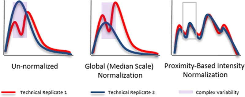
Further investigating this CPTAC data reveals shortcomings in current normalization strategies. Examining the extracted chromatograms plots (XCs), each representing all peptide signals in a run (Experimental Procedures), reveals a trough in replicate 2 (REP 2) (Figure 1a) corresponding to the same time frame as the observed electrospray instability in the TIC generated from the raw data (Supplemental Figure 1 in the Supporting Information). Ideally, normalization would produce nearly identical XCs between replicates. Unfortunately, global scaling functions fail to mitigate complex variability (Figure 1b). Furthermore, global normalization can have unintended consequences and can adversely affect regions where no complex variability exists. Figure 1b shows that two regions of the XC for REP 2 now have more extraneous variability than before normalization, potentially disguising true biological variation.

Figure 1.

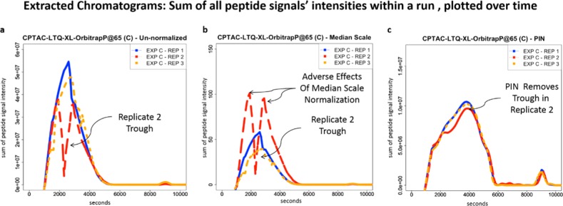
Complex variability in technical replicates. Extracted chromatograms (Experimental Procedures) from three HPLC–ESI–MS/MS technical replicates (CPTAC Study 6, LTQ-XL-OrbitrapP@86) show that even well-controlled HPLC–ESI–MS/MS experiments are vulnerable to complex variability. (a) Extracted chromatogram for Sample C’s replicate 2’s un-normalized data (EXP C – REP 2, long-dashed red line) contains a distinctive trough during the same time frame as the electrospray instability in its corresponding TIC (Supplemental Figure 1 in the Supporting Information). (b) Same data normalized by median scale result in extracted chromatograms where the distinctive trough remains. Extracted chromatograms for replicates 1 and 3 (EXP C – REP 1, solid blue line, and EXP C – REP 3, short-dashed orange line) only slightly diverge. However, replicate 2’s (EXP C – REP 2, long-dashed red line) extracted chromatograms show that the complex variability is now exaggerated, showing the adverse effects of median scale normalization. (c) Same data normalized by PIN result in similar extracted chromatograms for each of the three replicates. PIN removes the trough in replicate 2 (EXP C – REP 2, long-dashed red line). This demonstrates PIN’s ability to mitigate complex variability.

In response to the shortcomings of current normalization strategies exemplified in this data from CPTAC, we developed proximity-based intensity normalization (PIN), which mitigates complex variability and systematic bias in MS1 chromatographic data. Here we describe the underpinnings of this strategy and demonstrate that PIN improves repeatability and reproducibility, allowing researchers to better detect biological variation from biological MS data.

Experimental Procedures

Saliva Sample Collection and Processing

We collected and processed salivary endogenous peptides as previously described.¹⁵ In brief, we collected all saliva samples according to protocols approved by the University of Minnesota Institutional Review Board. Donors declared that they were healthy nonsmokers and were free of confounding conditions.

Endogenous Peptide Isolation

Clarified saliva was prepared from fresh whole saliva samples by centrifuging at 3000g at 4 °C for 15 min, followed by 16 100g at 4 °C for 1 min. The supernatant was mixed in a 10:1 ratio with denaturing buffer consisting of 4% SDS, 100 mol/L dithiothreitol, and 100 mmol/L Tris, pH 7.4. The samples were boiled for 5 min, cooled to room temperature, then added to a centrifugal filter (Amicon Ultra, 0.5 mL, 10 kDa, Millipore). Two hundred microliters of buffered urea (8 mol/L urea with 100 mmol/L tris pH 8.5) was added to the sample, and the mixture was centrifuged at 14 000g at room temperature for 40 min. An additional 200 μL of buffered urea was added, and the sample was centrifuged at 14 000g at room temperature for 40 min. The filters were discarded, and the collected peptides were alkylated, by the addition of iodoacetamide in buffered urea to 50 mmol/L in the dark for 20 min. MCX (Oasis 3 cc, 60 mg, Waters) cleanup was performed by diluting the samples to 3 mL with 2% formic acid and H₂O to pH ≤3. The MCX columns were equilibrated with 2 mL of 1:1 methanol: water followed by the addition of the entire sample, then washed with 3 mL of 0.1% formic acid and 2 mL of methanol; peptides were eluted with 1 mL of 95% methanol/5% ammonium hydroxide. The eluted peptides were dried in a speed-vacuum, redissolved in water, and quantified by a modified BCA assay (Thermo Scientific, Waltham, MA) using trypsin-digested saliva as a standard. Three micrograms of peptides were further purified and concentrated using the STAGE-tip protocol.¹⁶

Instrument Variability Experiment Sample Preparation

Fresh saliva was collected from a single donor and processed for isolation of endogenous peptides. Sufficient sample quantity was loaded in a single autosampler vial to run three replicate injections in succession.

Sample Variability Experiment Sample Preparation

Fresh saliva was collected from a single donor and divided into three portions. Each aliquot was processed for endogenous peptide isolation with the identical protocol, placed into individual autosampler vials and analyzed in succession.

Serial Dilution Experiment Sample Preparation

Fresh saliva was collected from a single donor and processed for isolation of endogenous peptides and aliquoted with increasing amounts (0.5, 1.0, 1.5, 2.0, 2.5, and 3 μg) into individual vials. Five hundred fmol of bradykinin was added to each vial.

HPLC–ESI–MS/MS

We analyzed the resulting peptide mixtures by online HPLC–ESI–MS/MS on an LTQ-Orbitrap XL mass spectrometer (Thermo Scientific, Waltham, MA) equipped with an Eksigent (Eksigent Technologies, Redwood City, CA) 1DLC nanoflow system and a MicroAS autosampler. An in-house, pulled tip capillary column with a 100 μm inner diameter was packed to 13 cm with Magic C18AQ 5 μm, 200 Å pore particles (Michrom Bioresources). Peptide mixtures were dissolved in an aqueous solution containing 2% ACN with 0.1% formic acid and then separated by a 2–40% ACN gradient in 0.1% formic acid over 60 min at 250 nL/min. Full-scan mass spectra were acquired in the Orbitrap at 60 000 resolution at m/z 400, followed by tandem mass spectrometry (MS/MS) in the LTQ of the five most intense ions from the full scan. Further details of the mass spectrometer settings were previously reported.¹⁵

Clinical Proteomic Tumor Analysis Consortium Study 6

National Cancer Institute’s CPTAC network’s Study 6¹⁴ data set LTQ-XL-OrbitrapP@65, which was downloaded from Tranche, is now available at https://cptac-data-portal.georgetown.edu/cptac/public. Because data acquisition for this study was performed in profile mode, we converted the .raw files to mzXML files using msConvert version 3.0.3364 specifying centroid = true.

Peptide Signal Extraction

Peptide signals were extracted using an in-house software application. In brief, the software takes in a list of mzXML files and processes the file sequentially. Each mzXML file was processed scan by scan. First, monoisotopic peak clusters were detected and deisotoped. Second, after all scans were processed, extracted ion chromatograms (XICs) were constructed from the deisotoped peaks. Next, peptide signals were then constructed from XICs. The peptide signals’ m/z values and retention times were adopted from the XIC’s apex peak. In lieu of computing an XIC’s area under the curve, a peptide signal’s intensity was computed by summing its XIC peak intensities. (Note that XICs were truncated to eliminate the exceedingly trailing chromatographic peaks. We arbitrarily selected 2 min from the XICs apex peak.) Finally, corresponding peptide signals were grouped across multiple analyses based on m/z and retention time tolerances. As a quality measure, we required at least two MS2 scans (among all sequentially analyzed files) corresponding to each peptide signal. This software and Thermo .raw files used for analyses are available from the authors upon request.

Protein and Peptide Identification

All MS/MS data were analyzed using Sequest version 27, rev 12 (Thermo Scientific). The steps for searches are described. First, we downloaded the yeast Uniprot FASTA database (ftp://ftp.uniprot.org/pub/databases/uniprot/current_release/knowledgebase/proteomes/YEAST.fasta.gz, February 3, 2012) and the cRAP contaminant FASTA database (downloaded from ftp://ftp.thegpm.org/fasta/cRAP, February 28, 2012). The cRAP UPS entries were replaced with entries from an updated UPS FASTA database (http://www.sigmaaldrich.com/life-science/proteomics/mass-spectrometry/ups1-and-ups2-proteomic.html, February 22, 2012). The YEAST and cRAP FASTA databases were concatenated and designated as the forward database. Each protein sequence was then reversed with a perl script (Matrix Science, Boston, MA), designated as the decoy database, and concatenated to the forward database. The resulting database contained 13 532 proteins. For the C versus E experiment, Sequest parameters included a fragment ion mass tolerance of 1 Da, oxidation of methionine as a variable modification, and 2 Da mass tolerance.

Scaffold version 3.6.1 (Proteome Software, Portland, OR) was used to validate MS/MS-based peptide and protein identifications. Peptide identifications were accepted if they met minimum criteria 7 ppm precursor mass tolerance, one tryptic terminus minimum, six amino acid minimum length, and 90.0% probability as specified by the Peptide Prophet algorithm.¹⁷ Protein identifications were accepted if they could be established at >80.0% probability (Protein Prophet)¹⁸ and contained at least one identified peptide. Proteins with similar peptides that could not be differentiated based on MS/MS analysis alone were grouped to satisfy the principles of parsimony. The resulting false discovery rate (FDR) within Scaffold was 1.4% at the protein level and 0.1% at the peptide level (Supplemental Files 1 and 2 in the Supporting Information).

Statistical Analysis

Unless otherwise specified, all statistical analyses were performed using the R statistical package, version 2.14-0 2011-10-31, R.app 1.41 or 3.02 2013-09-25. Two sample t tests were conducted using the R function t.test and the default confidence level was 0.95. Prior to multivariate analyses, for example, pooled estimate of variance, data were first log-transformed to obtain a normal distribution prior to computing variance.

Extracted Chromatograms

We generated XCs by first determining each peptide’s XIC and then summing their recorded intensities within each scan. The resulting summed intensities (y axis) were plotted over time (x axis) using R’s lowess function (locally weighted polynomial smoother); the smoothing span parameter set to 0.07 for Figure 4 and 0.05 for Figure 6. All other lowess default parameters were accepted.

Figure 4.

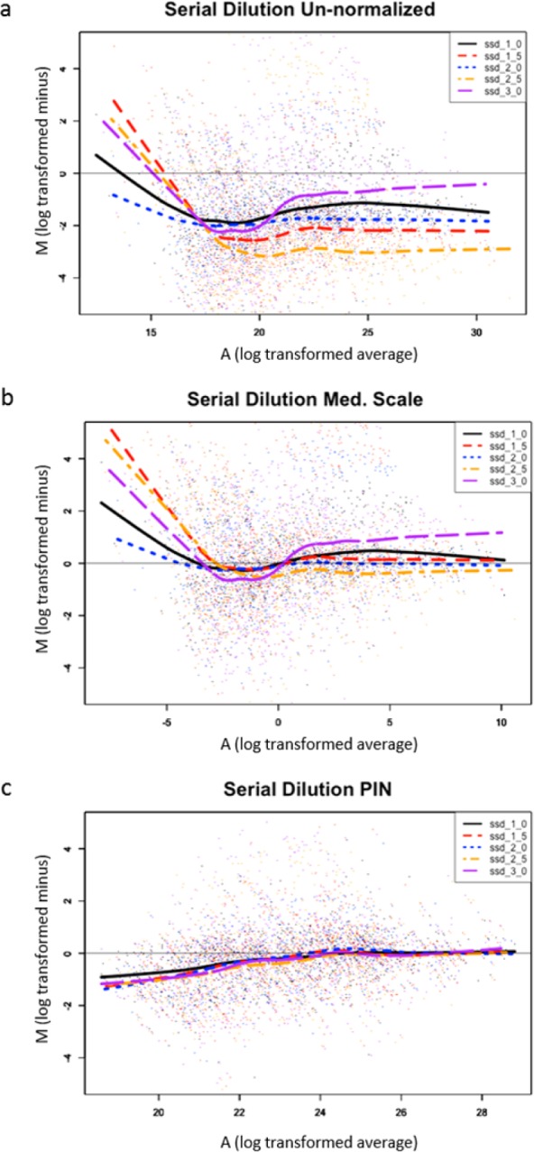
Serial dilution - PIN versus median scale minus versus average (MA) pots. (a) MA plot visually demonstrates that PIN outperforms median-scale normalization in mitigating systematic bias. (a) MA plot of un-normalized data for six different loading amounts reveals systematic bias (regression lines diverge from y = 0). (b) MA plot of median scale data for six different loading amounts demonstrates a slight improvement in systematic bias (regression lines begin to converge around y = 0). (c) MA plot for PIN normalized data for six different loading amounts demonstrates a substantial improvement in systematic bias (regression lines converge around y = 0).

Figure 6.

Peptide signal extracted chromatograms PIN versus spiked-in standard normalization for six different loading amounts. (a) Un-normalized extracted chromatogram plot shows systematic bias. (The 2.0 and 3.0 μg extracted chromatograms are not in the correct order.) (b) Spiked-in (bradykinin) normalized extracted chromatogram plots show that the 2.0 μg extracted chromatogram is now above the 1.0 μg extracted chromatogram but is still below the 2.0 μg extracted chromatogram. (c) PIN normalized extracted chromatogram shows convergence, indicating the removal of systematic bias. (d) Scaling PIN normalized data by the original loading amounts plot shows extracted chromatograms monotonically increasing and in the correct order.

Current Normalization Strategies

Linear Regression

Linear regression normalization was performed by applying least-squares regression on minus versus average (MA) scatter plots using a pairwise iterative algorithm.^5,6 First, the algorithm selected peptide signals using the CWS method and then MA-transformed peptide signal intensities for each pair of runs using eqs 1 and 2 in Supplementary Note 2 in the Supporting Information. Fitted data were generated in R with the function lm, for example, lm(m∼a), and subtracted from observed ratios with eq 3. The data then were deconvoluted using eq 4 in Supplementary Note 2 in the Supporting Information. We performed the iteration process twice because the difference between the mean of all intensity ratios from the previous iteration was <0.005, as previously described.⁶

Loess

Author: Loess normalization was performed in R using the normalizeCyclicLoess function found in the limma package.¹⁹ The algorithm first selected peptide signals using the CWS method; next, the algorithm selected log₂ transformed intensities (as required by normalizeCyclicLoess) prior to submitting them to normalizeCyclicLoess using default parameters. The algorithm returned results to their nonlog scale.

Quantile

Quantile normalization was performed in R using the normalizeQuantile function found in the limma package.¹⁹ The algorithm selected peptide signals using the CWS method prior to normalizedQuantile analysis with default parameters.

Reference Run

Normalization was performed by selecting a single run as a reference. Peptide signal intensities for all nonreference data were normalized to the reference run. The algorithm first selected signals using the CWS method prior to computing the median of peptide signal intensity ratios, which was used as a normalization factor.⁶ The first replicate was arbitrarily selected as the reference run.

Median Scale (Central Tendency)

Median scale was performed by scaling peptide signal intensities values within each run by the median of peptide signals selected using the CWS method.

PIN Neighborhood Construction

While we mathematically define PIN’s neighborhood construction (see Results and Discussion), in practice we define a peptide signal’s neighborhood boundary using a retention time window around the peptide signal’s retention time (Figure 2). The retention time window can be static or dynamic. A static retention time window is centered at the peptide signal’s retention time, plus and minus a specified time period, for example, 2 min. A dynamic retention time window is based on the width of a peptide signal’s XIC. Once the neighborhood boundaries are established, the neighborhood is then populated with all peptide signal XIC peaks within the retention time window. A peptide signal’s intensity is then normalized by computing the proportion of signal within the neighborhood. The proportion is computed by dividing the peptide signal’s intensity by the sum of neighborhood XIC peak intensities. For all analyses discussed herein, neighborhood boundaries were determined by a dynamic retention time window corresponding to the peptide signal’s XIC width.

Figure 2.

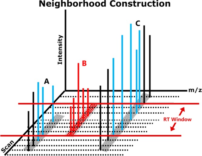
PIN’s neighborhood construction. XICs for three peptide signals (A–C) are shown in three dimensions. Here peptide signal B’s neighborhood boundaries (RT window depicted by the horizontal red lines) are determined by its XIC width. Peptide signal B’s neighborhood construction includes all XIC peaks within its retention time window (peaks in red and blue). In this case, the neighborhood includes a portion of peptide signals A’s XIC and a portion of peptide signal B’s XIC.

Results and Discussion

Overview of the PIN Strategy

In PIN, we take a nontraditional approach. We observe that complex variability, such as ESI instability, affects bounded temporal regions within chromatographic data, as opposed to systematic bias which affects the entire HPLC–ESI–MS/MS run. Therefore, to mitigate complex variability, PIN normalizes each peptide signal’s intensity by computing its proportion of intensity relative to its neighboring peptide signals (Figure 2).

Mathematically, we define a peptide signal’s neighborhood as

where N is the set of neighboring peptide signals, n is a peptide signal, rt_min is the index of the peptide signal corresponding to the neighborhood’s lower retention time boundary, and rt_max is the index of the peptide signal corresponding to the neighborhood’s upper retention time boundary. With the neighborhood defined, a peptide signal’s normalized intensity, that is, its proportion of neighborhood intensity, is

where n_j is the intensity of peptide signal j and n_i is the intensity of peptide signal i falling within the neighborhood retention time boundaries.

The premise for this new approach is that we view biological samples and HPLC–ESI–MS/MS chromatographic data as compositional. Mathematically, a composition is defined as “... x of D parts is a D x 1 vector (x₁, x₂, ..., x_D) of positive components whose sum is 1”.(20) Because the components’ quantities must sum to 1, compositional data are an example of sum-constrained data.²¹ While the concept of sum-constrained data may seem foreign to most, sum-constrained data are actually quite prevalent. For example, simple percentages and parts per million (ppm) are sum-constrained measurements. Percentages are sum-constrained because the total is constrained to 100, and ppm measurements are sum-constrained because the total is constrained to one million.^20,22

In analyzing compositional data, statistical analyses must be done with care because naïve analysis of compositional data can lead to incorrect inferences.²³ This is because compositional data loses its absolute abundance information. The only abundance information that remains for a single component is relative to the other components making up the whole.²¹ In other words, a component’s abundance is its proportion to the whole. Prior to statistical analyses, compositional data must meet two conditions: (1) the components of interest must be relatively small parts of the whole; (2) components within the whole must remain relatively constant in size and composition.²² When these conditions are met, univariate statistical tests, such as a student’s t test, on compositional data should not lead to incorrect inferences.²²

The rationale for our treatment of biological samples as compositions is two-fold. First, biological systems, whether at the molecular, cellular, or organ level, are dynamic and interactive. For example, within a proteome, the presence, absence, or change in abundance of one or more proteins can affect the presence, absence, or change in abundance of one or more other proteins in the system. Therefore, the abundance of a particular protein, relative to other proteins is important. As a result, researchers reveal biological variation by finding differences in a biological sample’s composition.²⁴ Second, sample collection and preparation impose constraints on the number of proteins available for measurement.^20,22 For example, aliquoting a portion of a sample, perhaps based on a Bradford assay, puts a cap on the amount of protein used for comparison. As a result, we deem biological samples as compositional.

The rationale for our treatment of chromatographic data as compositional stems from the fact that constraints are imposed within HPLC–ESI–MS/MS workflows. For example, during ESI, coeluting peptides compete for a finite number of charges and a limited space on droplets.^25,26 The finite number of charges and the limited space are constraints. As a result, mass spectral intensities of ionized peptides depend on their coeluting peptides,²⁷ and thus we deem the resulting chromatographic data are compositional.

Therefore, when we treat chromatographic data resulting from the analysis of proteomic samples as compositional, we can detect statistically significant differences in proportions across populations. This compositional data meets the two prerequisite conditions for its statistical analysis: (1) the amount of a single component (peptide) is small relative to the whole, which remains true in its corresponding chromatographic data, and (2) in the vast majority of biological systems, the core proteome and its digested peptides, accounts for more than 90% of the measured protein mass in a sample; that is, only 10% is compositionally different between similar biological samples.²⁸ This also remains true in the corresponding chromatographic data. Thus, when we view complex biological samples and chromatographic data as compositional, we can use simple univariate statistics (such as student’s t test) to reveal biological variation.

We also reason that temporal regions within in chromatographic data generated by HPLC–ESI–MS/MS workflows are subcompositions. This reasoning stems from the fact that when using the same (or very similar) LC column, peptides elute in approximately the same order.²⁹ As a result, retention time windows within resulting chromatograms will contain approximately the same set of peptide signals when analyzing different samples with overall similar composition. Thus, this region becomes a subcomposition, which, for mathematical purposes, is just another composition. We can do so even when complex variability is present because complex variability similarly affects peptide signal intensities within close temporal proximity.

Finally, when we view regions (also called neighborhoods) of chromatographic data as compositional, we can detect statistically significant differences in peptide signal proportions across populations. This is true because the data again meet the two prerequisite conditions for comparisons of compositional data: (1) provided that neighborhood boundaries are properly set, a peptide signal’s neighborhood population is large enough so that the intensity of a peptide signal remains small relative to the sum of its neighbors’ intensities and (2) provided that similar LC (column type and gradient duration) is used, neighborhoods will contain sufficiently overlapping populations.

With underlying assumptions as a basis, we assessed our PIN strategy’s ability to mitigate systematic bias and complex variability and reveal statistically significant biological variation.

Results

As an initial evaluation, we applied PIN to the CPTAC data described in the Introduction – data that alluded to the capabilities of global scaling functions and motivated our development of a new method. Use of PIN on this data produced the ideal result expected from normalization (Figure 1c): nearly identical XCs between replicates, even for the run containing the complex variability due to electrospray instability. Encouraged by these results, we further evaluated PIN vis-à-vis median scale and other current normalization strategies. We applied several different peptide selection strategies and global scaling functions to archived data sets from four experiments: Instrument Variability, Sample Variability, Serial Dilution (as a proxy for loading amount differences), and CPTAC Study 6. The results of these experiments, when taken together, demonstrate PIN’s superior mitigation of systematic bias and complex variability while retaining biological variability.

Reduction in CV and PEV

To assess reduction in instrument variability, we generated three replicates by analyzing a single aliquot of salivary endogenous peptides using an autosampler and HPLC–ESI–MS/MS three times consecutively. (See Experimental Procedures and Supplemental Tables 3 and 4 in the Supporting Information.) First, we assessed reduction in variability between un-normalized data, data normalized by five global scaling functions, and data normalized by PIN. We used two commonly employed metrics: pooled estimate of variance (PEV) and median standard deviation coefficient of variance (CV). Although we evaluated numerous scaling functions,^5,6 we only report PIN and the five best performing normalization strategies determined by PEV and CV reduction. For the global scaling functions, we employed the CWS peptide selection strategy prior to normalization. For PIN, we employed the CWS peptide selection strategy after normalization. Results are shown in Figure 3. In the instrument variability experiment, PIN outperformed the five best current normalization strategies by reducing PEV by 73% and CV by 46%, compared with an average of 13 and 19% respectively for the global scaling functions.

Figure 3.

PIN versus five current normalization strategies. Four experiments show PIN’s superior performance in reducing variance using two commonly used measurements: pooled estimate of variance (PEV) and coefficient of variation (CV). (a,c) PIN (right-most column in each figure) versus five common normalization strategies in reducing PEV for each of the four experiments. (b,d) PIN (again, right-most column in each figure) versus the same five common normalization strategies in reducing CV for each of the four experiments.

To assess reduction in the variability resulting from sample handling, we followed the same protocol as the instrument variability experiment, except we prepared three aliquots of salivary endogenous peptides in parallel and analyzed each aliquot using an autosampler and HPLC–ESI–MS/MS. (See the Experimental Procedures and Supplemental Tables 5 and 6 in the Supporting Information.) Again, we employed CV and PEV and compared PIN’s results to the top five performing normalization strategies. PIN continued to outperform these normalization strategies by reducing PEV by 71% and CV by 41% compared with an average of 11 and 8%, respectively, for global scaling functions.

To assess reduction in variability resulting from loading amount differences, we conducted serial dilution experiments using a complex mixture of salivary endogenous peptides and bradykinin as a spiked-in standard. (See the Experimental Procedures and Supplemental Tables 7 and 8 in the Supporting Information.) Traditionally, researchers have conducted serial dilution experiments to determine peptide abundances in a concentrated sample or produce calibration curves. We used serial dilution experiments unconventionally, as a proxy for loading amount differences We prepared six aliquots of this mixture by combining increasing amounts (0.5, 1.0, 1.5, 2.0, 2.5, and 3.0 μg) of salivary endogenous peptides with an equal amount of bradykinin (50 fmol). We then analyzed the six mixtures via HPLC–ESI–MS/MS. We again employ PEV and CV and compared PIN to the top five performing normalization strategies. PIN reduced PEV by 75% and CV by 55% compared with an average of 34 and 23%, respectively, for global scaling functions.

To assess reduction in variability in the face of biological variation, we used data from the CPTAC Study 6 data set for instrument aliased LTQ-XL-OrbitrapP@65. In brief, CPTAC Study 6 evaluated mixtures of yeast with Sigma UPS1 spiked in at five different levels (A–E), each level three times greater than the previous level.¹⁴ Each sample was then analyzed three times by HPLC–ESI–MS/MS. We selected samples C and E because sample C contained complex variability and sample E contained nine times the amount of UPS1 (Experimental Procedures, Supplemental Tables 9 and 10 in the Supporting Information). Using the C versus E data set, PIN again outperformed global scaling function PIN reduced PEV by 61% and CV by 19% while global scaling functions, on average, PEV by 9% and surprisingly increased CV by 14% (Figure 3d, fourth row). In this case, global scaling functions had a negative effect rather than a positive effect in normalizing intensities.

PIN and Systematic Bias Mitigation

To assess PIN’s ability to mitigate systematic bias, we employed MA plots. Again, we used the serial dilution data set as a proxy for loading amount differences. We chose to visualize loading amount differences because it was a classic example of systematic bias (Figure 4 and Supplementary Figure 2 in the Supporting Information). When we plotted the un-normalized peptide signal intensities, we observed divergent regression lines, indicative of systematic bias due to loading amount differences (Figure 4a). As described in Supplemental Note 1 in the Supporting Information, data with no systematic bias would result in regression lines lying on the horizontal line positioned at 0 on the y axis. We then plotted the same data after normalization using median scale as the global scaling function (Figure 4b). We observed that the regression lines have slightly converged and were repositioned below and above y = 0, indicating improvement in systematic bias. Finally, we plotted the data after normalization using PIN (Figure 4c). We observed that the regression lines on the right end of the plot were then positioned on or very near y = 0. However, we also noted that the lines remained below the horizontal flat line on the left end of the plot. Unlike median scale, the regression lines converged, making the regression lines nearly indistinguishable. From these observations, we concluded that using PIN performed well to mitigate the systematic bias, although a small amount remains. Furthermore, we concluded that PIN outperformed median scale normalization in making systematic bias consistent between runs.

Absolute Abundance, Relative Abundance, and Compositional Measurements

Typically, in a serial dilution experiment, the data are normalized using an internal or spiked in peptide with the goal of determining absolute abundance and relative abundance, rather than composition. The standard metric for absolute abundance is the coefficient of correlation (R²), with the goal of perfect correlation (R² = 1.0). The standard metric for relative abundance is fold change, with the goal of monotonically increasing fold changes corresponding perfectly to the original amounts loaded. Here we expected fold changes of 0.5, 1.0, 1.5, 2.0, 2.5, and 3.0 corresponding to the saliva peptide load amounts of 0.5, 1.0, 1.5, 2.0, 2.5, and 3.0 μg, respectively.

We first plotted the un-normalized intensity for a single salivary peptide (GPGIFPPPPPQP), indicative of other salivary peptides found in each of the six serial dilution runs and computed the R² and fold changes (Figure 5a,e). We noted that R² = 0.81, and fold changes were compressed and not monotonically increasing. We then plotted the spike-in normalized intensity (with 500 fmol bradykinin peptide) of the same peptide and computed the R² and fold changes (Figure 5b,e). The measured correlation improved to R² = 0.98, and the fold changes were now monotonically increasing.

Figure 5.

PIN versus spiked-in standard normalization for a single peptide (GPGIFPPPPPQP) intensity with six different sample loading amounts. (a) Un-normalized intensity plot shows mediocre correlation (R² = 0.82). (b) Spiked-in (bradykinin) normalized intensity plot shows improved correlation (R² = 0.98) but does not remove systematic bias stemming from loading amount differences (slope is very high). (c) PIN normalized intensity plot shows decreased correlation (R² = 0.81) but removes systematic bias stemming from loading amount differences (slope = 0.01). (d) PIN normalized data followed by original loading amount scaling shows improved correlation (R² = 0.99), which is better than spiked-in standard normalization. (e) Table showing fold changes for each intensity plot (a–d) using the 1.0 μg sample loading amount as the common denominator, while PIN compresses the fold changes.

However, when we use the serial dilution experiment as a proxy for loading amount differences, then, our goal should not be to achieve perfect correlation to absolute amounts; rather, our goal is to find no compositional differences (slope = 0.0). This stems from the fact that even though overall loading amounts varied between these samples, within each sample the proportion of any given peptide to the whole did not change because overall composition did not change. When considering composition, a flat line indicates no systematic bias. Furthermore, relative fold changes should all be equal to 1, indicating no changes in the composition. We plotted the PIN-normalized intensities for the same peptide and computed the slope and fold changes (Figure 5c,e). We observed that normalizing with PIN achieves a slope = 0.01, and fold changes are near 1, indicating little change in biological variation.

Because we knew the loading amounts, we estimated the absolute abundance of peptides initially loaded onto the HPLC column by scaling PIN normalized intensities by the run’s loading amount. Scaling PIN normalized data by the loading amount showed R² = 0.99 (Figure 5d) and monotonically increasing fold changes (Figure 5e). We also observed fold changes were compressed. In this case, scaled PIN outperformed spike-in normalization for estimating absolute peptide abundance and in estimating fold changes.

We next turned our attention from a single peptide fold change to the analysis of composite XCs representing all peptide signals in a run. When we plotted the un-normalized XCs, we observed a clear separation of monotonically increasing XCs, indicating the presence of systematic bias (Figure 6a). However, upon closer inspection, we found that the XCs for the 2.0 μg and 3.0 μg samples were not in the expected order. (The 2.0 μg XC lay above the 3.0 μg XC.) We then plotted the spike-in normalized XC and observed that the 3.0 μg XC shifted its position but still lay below the 2.0 μg XC (Figure 6b). Next we plotted the XCs for the PIN normalized data and observed a convergence of the XCs (Figure 6c). Furthermore, we observed an undulation in the XCs, consistent across the different runs. Finally, we plotted the PIN normalized data scaled by loading amounts and observed that the XCs became monotonically increasing and were in the correct order for nearly all time points (Figure 6d), with the exception of the lowest loading amounts.

Detecting Biological Variation

Finally, we assessed PIN vis-à-vis common normalization strategies in the context of detecting of biological variation. Again, we used the CPTAC Study 6 and selected samples C and E. Here we used a student’s t test to determine the number of differentially abundant (or proportional) UPS1 and yeast proteins and peptides found.

We used SPANS¹⁰ to recommend and perform the optimal peptide select strategy and global scaling function combinations. SPANS performed correctly, finding no global scaling functions were appropriate for the CPTAC C versus E data set. These results confirmed our previous findings that global scaling functions cannot capture and mitigate complex variability. Nonetheless, SPANS was run using three normalization strategies: (1) LOS (5%) peptide selection strategy with mean global scaling; (2) RIP peptide selection strategy with mean global scaling; and (3) RIP peptide selection strategy with median global scaling (Supplemental Table 11 in the Supporting Information). We compared SPANS results to PIN normalized results (Figure 7).

Figure 7.

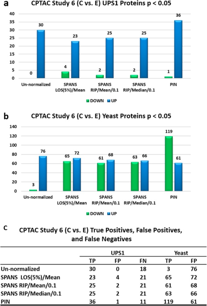
CPTAC C versus E statistically different UPS1 and yeast proteins. The UP designation indicates proteins present lower abundance (or proportion for PIN) in sample E compared with sample C. The DOWN designation indicates lower abundance (or proportion in PIN) in sample E compared with sample C. (a) UPS1 proteins statistically different between samples C and E. (b) Yeast proteins that are statistically different between samples C and E. (c) Number of true positives, false-positives, and false-negatives for UPS1 and yeast proteins.

PIN outperformed median and mean global scaling functions in finding statistically significant UPS1 proteins (Figure 7a). With PIN, we found 36 statistically different UPS1 proteins going up (true positives) and only 1 UPS1 protein going down in E versus C (false-positive). Global scaling functions performed abysmally, finding fewer UPS1 proteins as statistically different compared with the un-normalized data. PIN found 20% more (6) UPS1 proteins as statistically different that were false negatives in the un-normalized data (Figure 7c).

One important point is that when we treat chromatographic data as compositional data, we also measure statistically significant decreases in background yeast proteins in sample C versus E. We assert these are true positives, reflecting physical realities of these samples. Our reasoning is that when viewing the proteome as compositional, then it follows that as the proportion of UPS1 proteins goes up, the proportion of yeast proteins must go down. It is also well known that increasingly abundant peptides can suppress ionization of coeluting peptides,^30,31 leading to decreased proportional intensities of some yeast peptides in response to increasing load of UPS1 peptides. This may be even more prevalent an affect within adding relatively large amounts of the UPS1 standard into the yeast background. Therefore, with PIN, we expect to find a larger number of yeast peptides with reduced proportion to the whole when compared with other scaling functions (Figure 7b,c).

Discussion

To our knowledge, we are the first to demonstrate that biological variation can be revealed in proteomic chromatographic data by viewing it as compositional. Here we also introduce PIN, a new local method that normalizes a peptide signal’s intensity by computing its proportional intensity relative to its neighborhood. We show that PIN dominates competing normalization strategies when measuring reduction in variability and finding biological variation, even when complex variability is present.

The only related work is very recent work by Lyutvinskiy et al., which describes a new instrumental response correction method, a local normalization method, for significant variations in the eluent and analyte composition for improving accuracy of predictive models.³² We compared and contrasted PIN with their method and found some similarities and some striking differences. Both methods employ temporally bounded neighborhoods to normalize each peptide signal. However, the composition of the neighborhoods is decidedly different in the two methods. While PIN takes an unbiased approach to populating its neighborhood by including all peptide signal XIC peaks within a retention time window, their method takes a biased approach by populating their neighborhoods using only peptides confidently identified from MS2 spectra. Furthermore, the method for correction is not clearly defined, making it difficult to evaluate. In one instance, they describe an abundance alignment method using unchanged peptides as internal standards. In another instance, they report using the square root of the median of all peptides within the retention time window. Unfortunately, their report did not evaluate performance vis-à-vis common normalization strategies, making it difficult to compare to our PIN strategy. They did report that their normalization strategy improved their predictive model, but it is unclear to us whether the improvement stemmed from the local nature of their strategy or if other common normalization strategies would have produced similar results. Regardless of the differences, we both agree on the central need to account for complex variability in intensity-based quantification.

A key benefit of PIN over common normalization strategies is its simultaneous mitigation of multiple types of measurement error, including systematic bias and complex variability. This benefit stems from treating chromatographic data as compositions and temporal regions within the data as subcompositions. Thus, any bias affecting the composition as a whole will also affect subcompositions. As a result, when PIN mitigates complex variability within the subcomposition, it inherently also mitigates systematic bias.

A second benefit of PIN over common normalization strategies is that PIN requires no a priori knowledge of the type or source of measurement error. For example, a pipetting error doubling the amount of the sample does not necessarily correspond to a linear response in corresponding ion intensities in the resulting data. Therefore, simply normalizing by a single global scaling factor, such as the median of measured ion intensities, is not accurate. Computing the appropriate global scaling factor to mitigate systematic bias involves a priori knowledge of both absolute loading amounts and absolute ion counts. However, because PIN treats chromatographic data as compositional, the only information about peptide abundance and ion counts is relative information; thus, PIN requires no knowledge of absolute loading amounts or absolute ion counts.

A third benefit of PIN over common normalization strategies utilizing global scaling functions is that PIN does require a complete matrix on which to compute and thus implicitly handles the missing value problem. PIN simply requires a neighborhood populated with peptide signals. Then, to compare a single peptide signal’s PIN normalized intensities (proportions) across runs, its neighborhoods must be compositionally similar. If needed, missing values can still be imputed after normalization but prior to statistical inference, as is recommended.⁹

Of course, as with any method, PIN’s performance depends on some factors. First, PIN relies on high-resolution instrumentation and accurate mass measurements (<10 ppm error) to extract and quantify relevant chromatographic information. Fortunately, such systems are routinely available.³³ Second, as with other methods, the peptide elution order for analyzed mixtures must be similar; PIN requires similar order to form similar neighborhoods. This means mixtures analyzed using different types of chromatographic systems may not be easily compared. Third, although PIN tends to compress the dynamic range of fold changes, the end results are unaffected because it is fold change statistical significance (not numerical value) that counts for determining biological variation. However, if the original loading amount is known, for example, in a serial dilution experiment, that information can be used to scale results and accurately compute fold changes. Fourth, with any normalization method, overfitting and underfitting data is a concern. With PIN, we first construct neighborhoods using a temporal window, and the width of this window primarily controls data fitting quality. We conducted several experiments (results not shown) varying the window width and found that varying the window width between 2 to 5 min as well setting window size to the temporal width of a true peptide signal’s XIC made little difference in the results. However, setting the window <2 min and >5 min tended to overfit and underfit the data, respectively. We expect that optimal window width will correlate somewhat with chromatographic characteristics, primarily gradient duration. Therefore, we utilize the width of the peptide signal’s XIC as input to a function dynamically computing each peptide signal’s temporal boundaries.

Despite PIN’s improvements in reducing variability and the number of false-negatives reported, MS-based results must still be confirmed via hypothesis-driven experiments, such as a Western blot or targeted MS. Targeted MS, for example, SRM, is a powerful tool gaining popularity over traditional biochemical analyses due to the ever-increasing scale of today’s high-throughput experiments.¹³ Such experiments require as input a transition list or an inclusion list containing feature values (m/z – retention time pairs, which are simply peptide signals). Because PIN operates on a list of peptide signals, each with an associated MS/MS spectrum containing potential SRM transitions, the software implementing PIN could easily be extended to construct these lists. Thus, PIN is well-suited to drive targeted MS experiments.

Given that common normalization strategies cannot capture and correct systematic bias and complex variability inherently present in HPLC–ESI–MS/MS workflows, we expect PIN to dramatically improve intensity-based quantification from HPLC–ESI–MS/MS data. Furthermore, although we studied complex protein digests and endogenous peptide mixtures, we believe PIN will be widely applicable to many omics fields using HPLC–ESI–MS/MS to analyze complex mixtures, for example, lipidomics, glycomics, and metabolomics. The upshot will, we expect, be reproducibility- and repeatability-improved, and otherwise falsely reported or missed statistically significant biological variation will be discovered.

Supporting Information Available

Portion of the CPTAC Study 6C experiment’s chromatogram. Minus versus average reveals systematic bias. Minus versus average plots for four experiments: instrument variability, sample variability, serial dilution, and CPTAC Study 6 C versus E. variables and equations used in analysis. Peptide and protein reports. This material is available free of charge via the Internet at http://pubs.acs.org.

The authors declare no competing financial interest.

Funding Statement

National Institutes of Health, United States

References

- Cravatt B. F.; Simon G. M.; Yates J. R. 3rd. The biological impact of mass-spectrometry-based proteomics. Nature 2007, 4507172991–1000. [DOI] [PubMed] [Google Scholar]
- Bantscheff M. Mass spectrometry-based chemoproteomic approaches. Methods Mol. Biol. 2012, 803, 3–13. [DOI] [PubMed] [Google Scholar]
- Neilson K. A.; Ali N. A.; Muralidharan S.; Mirzaei M.; Mariani M.; Assadourian G.; Lee A.; van Sluyter S. C.; Haynes P. A. Less label, more free: approaches in label-free quantitative mass spectrometry. Proteomics 2011, 114535–53. [DOI] [PubMed] [Google Scholar]
- Tabb D. L.; Vega-Montoto L.; Rudnick P. A.; Variyath A. M.; Ham A. J.; Bunk D. M.; Kilpatrick L. E.; Billheimer D. D.; Blackman R. K.; Cardasis H. L.; Carr S. A.; Clauser K. R.; Jaffe J. D.; Kowalski K. A.; Neubert T. A.; Regnier F. E.; Schilling B.; Tegeler T. J.; Wang M.; Wang P.; Whiteaker J. R.; Zimmerman L. J.; Fisher S. J.; Gibson B. W.; Kinsinger C. R.; Mesri M.; Rodriguez H.; Stein S. E.; Tempst P.; Paulovich A. G.; Liebler D. C.; Spiegelman C. Repeatability and reproducibility in proteomic identifications by liquid chromatography-tandem mass spectrometry. J. Proteome Res. 2010, 92761–76. [DOI] [PMC free article] [PubMed] [Google Scholar]
- Callister S.; Barry R.; Adkins J.; Johnson E.; Qian W.; Webb-Robertson B.; Smith R.; Lipton M. Normalization approaches for removing systematic biases associated with mass spectrometry and label-free proteomics. J. Proteome Res. 2006, 52277–286. [DOI] [PMC free article] [PubMed] [Google Scholar]
- Kultima K.; Nilsson A.; Scholz B.; Rossbach U. L.; Falth M.; Andren P. E. Development and evaluation of normalization methods for label-free relative quantification of endogenous peptides. Mol. Cell. Proteomics 2009, 8102285–95. [DOI] [PMC free article] [PubMed] [Google Scholar]
- Ramanathan R.; Zhong R.; Blumenkrantz N.; Chowdhury S. K.; Alton K. B. Response normalized liquid chromatography nanospray ionization mass spectrometry. J. Am. Soc. Mass Spectrom. 2007, 18101891–9. [DOI] [PubMed] [Google Scholar]
- Jung S.; Effelsberg U.; Tallarek U. Microchip electrospray: cone-jet stability analysis for water-acetonitrile and water-methanol mobile phases. J. Chromatogr., A 2011, 1218121611–9. [DOI] [PubMed] [Google Scholar]
- Karpievitch Y. V.; Dabney A. R.; Smith R. D. Normalization and missing value imputation for label-free LC-MS analysis. BMC Bioinf. 2012, 13. [DOI] [PMC free article] [PubMed] [Google Scholar]
- Webb-Robertson B. J. M.; Matzke M. M.; Jacobs J. M.; Pounds J. G.; Waters K. M. A statistical selection strategy for normalization procedures in LC-MS proteomics experiments through dataset-dependent ranking of normalization scaling factors. Proteomics 2011, 11244736–4741. [DOI] [PMC free article] [PubMed] [Google Scholar]
- Karpievitch Y. V.; Taverner T.; Adkins J. N.; Callister S. J.; Anderson G. A.; Smith R. D.; Dabney A. R. Normalization of peak intensities in bottom-up MS-based proteomics using singular value decomposition. Bioinformatics 2009, 25192573–80. [DOI] [PMC free article] [PubMed] [Google Scholar]
- Wang P.; Tang H.; Zhang H.; Whiteaker J.; Paulovich A. G.; Mcintosh M. Normalization regarding non-random missing values in high-throughput mass spectrometry data. Pac. Symp. Biocomput. 2006, 315–327. [PubMed] [Google Scholar]
- Rudnick P. A.; Clauser K. R.; Kilpatrick L. E.; Tchekhovskoi D. V.; Neta P.; Blonder N.; Billheimer D. D.; Blackman R. K.; Bunk D. M.; Cardasis H. L.; Ham A. J.; Jaffe J. D.; Kinsinger C. R.; Mesri M.; Neubert T. A.; Schilling B.; Tabb D. L.; Tegeler T. J.; Vega-Montoto L.; Variyath A. M.; Wang M.; Wang P.; Whiteaker J. R.; Zimmerman L. J.; Carr S. A.; Fisher S. J.; Gibson B. W.; Paulovich A. G.; Regnier F. E.; Rodriguez H.; Spiegelman C.; Tempst P.; Liebler D. C.; Stein S. E. Performance metrics for liquid chromatography-tandem mass spectrometry systems in proteomics analyses. Mol. Cell. Proteomics 2010, 92225–41. [DOI] [PMC free article] [PubMed] [Google Scholar]
- Paulovich A. G.; Billheimer D.; Ham A. J.; Vega-Montoto L.; Rudnick P. A.; Tabb D. L.; Wang P.; Blackman R. K.; Bunk D. M.; Cardasis H. L.; Clauser K. R.; Kinsinger C. R.; Schilling B.; Tegeler T. J.; Variyath A. M.; Wang M.; Whiteaker J. R.; Zimmerman L. J.; Fenyo D.; Carr S. A.; Fisher S. J.; Gibson B. W.; Mesri M.; Neubert T. A.; Regnier F. E.; Rodriguez H.; Spiegelman C.; Stein S. E.; Tempst P.; Liebler D. C. Interlaboratory study characterizing a yeast performance standard for benchmarking LC-MS platform performance. Mol. Cell. Proteomics 2010, 92242–54. [DOI] [PMC free article] [PubMed] [Google Scholar]
- de Jong E. P.; van Riper S. K.; Koopmeiners J. S.; Carlis J. V.; Griffin T. J. Sample collection and handling considerations for peptidomic studies in whole saliva; implications for biomarker discovery. Clin. Chim. Acta 2011, 41223–242284–8. [DOI] [PMC free article] [PubMed] [Google Scholar]
- Rappsilber J.; Ishihama Y.; Mann M. Stop and go extraction tips for matrix-assisted laser desorption/ionization, nanoelectrospray, and LC/MS sample pretreatment in proteomics. Anal. Chem. 2003, 753663–670. [DOI] [PubMed] [Google Scholar]
- Keller A.; Nesvizhskii A. I.; Kolker E.; Aebersold R. Empirical statistical model to estimate the accuracy of peptide identifications made by MS/MS and database search. Anal. Chem. 2002, 74205383–92. [DOI] [PubMed] [Google Scholar]
- Nesvizhskii A. I.; Keller A.; Kolker E.; Aebersold R. A statistical model for identifying proteins by tandem mass spectrometry. Anal. Chem. 2003, 75174646–58. [DOI] [PubMed] [Google Scholar]
- Smyth G. K.Limma: Linear Models for Microarray Data. In Bioinformatics and Computational Biology Solutions Using R and Bioconductor; Gentleman R., Carey V., Dudoit S., Irizarry R., Huber W., Eds.; Springer: New York, 2005; pp 397–420. [Google Scholar]
- Lovell D.; Muller W.; Taylor J.; Zwart A.; Helliwell C.. Caution! Compositions!; Report Number EP10994; CSIRO Mathematical and Information Sciences: Canberra, Australia, 2010.
- Aitchison J. The statistical analysis of compositional data. J. R. Stat. Soc., Ser. B 1982, 139–177. [Google Scholar]
- Lovell D.; Müller W.; Taylor J.; Zwart A.; Helliwell C., Proportions, Percentages, PPM: Do the Molecular Biosciences Treat Compositional Data Right? In Compositional Data Analysis; John Wiley & Sons, Ltd: Hoboken, NJ, 2011; pp 191–207. [Google Scholar]
- Pawlowsky-Glahn V.; Buccianti A., Compositional Data Analysis: Theory and Applications. Wiley: Chichester, U.K., 2011; p xxi, 378 p. [Google Scholar]
- Aebersold R.; Mann M. Mass spectrometry-based proteomics. Nature 2003, 4226928198–207. [DOI] [PubMed] [Google Scholar]
- Kebarle P.; Tang L. From Ions in Solution to Ions in the Gas-Phase - the Mechanism of Electrospray Mass-Spectrometry. Anal. Chem. 1993, 6522A972–A986. [Google Scholar]
- Kebarle P.; Verkerk U. H. Electrospray: From Ions in Solution to Ions in the Gas Phase, What We Know Now. Mass Spectrom. Rev. 2009, 286898–917. [DOI] [PubMed] [Google Scholar]
- Tang K.; Page J. S.; Smith R. D. Charge competition and the linear dynamic range of detection in electrospray ionization mass spectrometry. J. Am. Soc. Mass Spectrom. 2004, 15101416–23. [DOI] [PMC free article] [PubMed] [Google Scholar]
- Nagaraj N.; Mann M. Quantitative Analysis of the Intra- and Inter-Individual Variability of the Normal Urinary Proteome. J. Proteome Res. 2011, 102637–645. [DOI] [PubMed] [Google Scholar]
- Hartman P. A.; Stodola J. D.; Harbour G. C.; Hoogerheid J. G. Reversed-phase high-performance liquid chromatography peptide mapping of bovine somatotropin. J. Chromatogr., A 1986, 3600385–395. [DOI] [PubMed] [Google Scholar]
- King R.; Bonfiglio R.; Fernandez-Metzler C.; Miller-Stein C.; Olah T. Mechanistic investigation of ionization suppression in electrospray ionization. J. Am. Soc. Mass Spectrom. 2000, 1111942–950. [DOI] [PubMed] [Google Scholar]
- Annesley T. M. Ion suppression in mass spectrometry. Clin. Chem. 2003, 4971041–1044. [DOI] [PubMed] [Google Scholar]
- Lyutvinskiy Y.; Yang H.; Rutishauser D.; Zubarev R. A. In Silico Instrumental Response Correction Improves Precision of Label-free Proteomics and Accuracy of Proteomics-based Predictive Models. Mol. Cell. Proteomics 2013, 1282324–31. [DOI] [PMC free article] [PubMed] [Google Scholar]
- Mann M.; Kelleher N. L. Precision proteomics: the case for high resolution and high mass accuracy. Proc. Natl. Acad. Sci. U. S. A. 2008, 1054718132–8. [DOI] [PMC free article] [PubMed] [Google Scholar]
Associated Data
This section collects any data citations, data availability statements, or supplementary materials included in this article.