Environmental heterogeneity affects the location of modelled communities along the niche–neutrality continuum

Abstract

The continuum hypothesis has been proposed as a means to reconcile the contradiction between the niche and neutral theories. While past research has shown that species richness affects the location of communities along the niche–neutrality continuum, there may be extrinsic forces at play as well. We used a spatially explicit continuum model to quantify the effects of environmental heterogeneity, comprising abundance distribution and spatial configuration of resources, on the degree of community neutrality. We found that both components of heterogeneity affect the degree of community neutrality and that species' dispersal characteristics affect the neutrality–heterogeneity relationship. Narrower resource abundance distributions decrease neutrality, while spatial configuration, which is manifested by spatial aggregation of resources, decreases neutrality at higher aggregation levels. In general, the degree of community neutrality was affected by complex interactions among spatial configuration of resources, their abundance distributions and the dispersal characteristics of species in the community. Our results highlight the important yet overlooked role of the environment in dictating the location of communities along the hypothesized niche–neutrality continuum.

1. Introduction

One of the fundamental questions in ecology is which rules drive the assembly of species in communities [1,2]. The niche theory [3] has been the focal explanation for many ecological patterns and processes, such as species distributions, species competitive interactions, community assembly and many more. However, some have argued that the high diversity of species of the same guilds in seemingly homogeneous ecosystems cannot be explained solely by niche processes [4,5]. In many cases, stochastic demographic processes and chance dispersal events play significant roles in structuring ecological communities. Hubbell's neutral theory of biodiversity [4] attempts to address the niche theory's limitations. The neutral theory demonstrates that simple mechanisms of demographic stochasticity (i.e. birth, death, migration and speciation of equivalent individuals of different species) can generate realistic biogeographic patterns, such as species abundance distributions, population size distributions, species–area curves and range size distributions, even when species are assumed to have identical niche requirements [6]. However, even Hubbell ([4], p. 24) acknowledged that ‘Actual ecological communities are undoubtedly governed by both niche-assembly and dispersal-assembly rules, along with ecological drift, but the important question is: What is their relative quantitative importance?’

The continuum hypothesis [7–10] emerged from an understanding that rather than being mutually exclusive, it is possible that the niche and neutral theories are located at opposite ends of a continuous axis that denotes the relative contributions of niche and neutral processes to the assembly of ecological communities. Accordingly, every community can be located at some point along this continuum, based on the relative contributions of niche and neutral processes to its composition. For example, tropical forest communities may be structured more by neutral processes compared with boreal forests, and as such may be located closer to the neutral end of the continuum axis [11]. While communities may be more or less neutral, no real-world community is truly neutral [6] or fully niche-based; thus, the ends of the niche–neutrality continuum exist only in theory [10].

A major limitation of the continuum theory is that it is difficult to assign real communities to specific locations along the niche–neutrality axis, because there are no direct ways to measure neutrality in real world communities. Measuring neutrality based on aggregate patterns (i.e. species abundance distributions) would be ineffective, because both niche and neutral processes can generate identical patterns [6,12,13]. Furthermore, although the neutral theory is sometimes described as being a null model to the niche theory [14], the amount of deviation of community structure from the predictions of null models that test the numbers of significant species co-occurrences [15] cannot serve as a measure of the niche–neutrality continuum, owing to the inherent differences between such null models and neutral models [14]. Also, the assumption underlying such null-model approaches—namely, that communities exhibiting species co-occurrence patterns that do not differ from random patterns (i.e. generated by null models) may be more neutral than communities that exhibit strong deviation from random structure—has been refuted. Communities generated by fully neutral processes can yield co-occurrence patterns that do differ from random ones, owing to dispersal limitations [16].

Given the difficulty in quantifying the continuum in real-world communities, experimental communities and virtual communities generated by mechanistic models remain the most promising approaches for evaluating the continuum theory. Model and analytical studies revealed that neutrality increases with species richness [8,17], species diversity [13] and speciation rate [11]. Presumably, there is little niche overlap in species-poor communities, and each species holds a large competitive advantage in locations that satisfy its habitat requirements. When species richness increases along a finite environmental gradient, there are three possible outcomes [18]: increased niche overlap, in line with the neutral theory; increased niche packing, in line with the niche theory; and increased niche space by either increasing axis length or number of niche axes. An increase in niche overlap increases the role of demographic stochasticity in determining community composition, because species no longer hold competitive advantages over other species with similar resource requirements [19]. Similarly, an increase in niche packing renders community assembly highly sensitive to stochastic events, because the differences in species’ niche requirements are smaller on average. Consequently, each species's ability to withstand demographic perturbations owing to stochastic processes is reduced, and the role of dispersal and chance colonization in structuring the community increases. Finally, an expansion of niche space may sustain the roles of niche processes in structuring communities as long as species can use the expanded niche space to enhance niche differentiation.

Besides the effect of increased species richness, there may also be extrinsic drivers that affect the location of communities along the continuum. One such possible driver is spatial heterogeneity of resources (hereafter environmental heterogeneity [20]). In the context of our study, we suggest that environmental heterogeneity comprises two components: spatially implicit abundance distribution of resource values in the environment and the spatial configuration of those resources (i.e. spatially explicit levels of aggregation across the environment, which is equivalent to spatial autocorrelation of resources [21]). Environmental heterogeneity affects many ecological patterns and processes, such as species abundance [22], species coexistence [23,24], species richness and community composition [25,26], and movement and dispersal of organisms [21,27–29]. Thus, by affecting propagule flow and establishment across landscapes, environmental heterogeneity may have an important effect on the location of communities along the niche–neutrality continuum. The presence of an organism at a given location depends on the degree to which the resource in that location is suitable for the establishment, survival and growth of the organism (which are all niche processes), as well as on the ability of the propagule to arrive in that location (which can be a neutral process). Therefore, we hypothesized that the location of a community along the continuum depends not only on its intrinsic characteristics (i.e. number of species and their niche characteristics), but also on the interaction of the niche and neutral processes that drive community dynamics, according to the heterogeneity of the environment.

Our objective was to quantify the direct effects of environmental heterogeneity on the location of communities along the niche–neutrality continuum in simulated ecological communities. Our secondary objective was to quantify the interacting effects of the two components of environmental heterogeneity together with species dispersal characteristics on the degree of community neutrality.

2. Material and methods

(a). The continuum model

To test our hypothesis regarding the relations between heterogeneity and the niche–neutrality continuum, we conducted a large number of simulations using an expanded version of an existing spatially explicit continuum model [8]. A brief description of the model follows, highlighting the alterations we made to fit the spatial nature of our research question (see [8] for a detailed description of the model). We developed the model in Python (http://www.python.org) and analysed the results using R v. 2.15.2 [30].

The model simulates the spatio-temporal dynamics of a virtual community based on a combination of niche and neutral processes. The community consists of adults and juveniles of different species, which reside in a landscape grid comprising 128 × 128 square and equal-sized cells. Each cell contains a single adult individual of a given species, and any number of juveniles of different species. The landscape grid denotes the values of a single environmental variable E, which ranges from 0 to 100. Outside the landscape that hosts the community, there exists a static regional species pool, which comprises the same species as in the local landscape and supplies a constant flux of propagules to each cell in the local landscape.

Individuals of different species differ in a single parameter: niche optimum (or niche centre). Each species has a niche optimum value which is within the range of the environmental variable E. Niche optimum values between 0 and 100 are assigned at random to each species at the beginning of the simulation. A second niche parameter, σ, denoting niche breadth, was identical for all species (σ = 5).

The model was built upon the following ecological processes, which occur at each time step in the following order. (1) Stochastic adult mortality. All individuals of all species have identical mortality probabilities at each time step. (2) Stochastic local dispersal of seeds/juveniles. Surviving adults generate propagules which disperse to their surrounding cells according to a two-dimensional dispersal kernel which is identical for all species:

2.1

where N_i is the number of propagules of species i arriving in cell (x, y) within a certain distance of an adult located at cell (x₀, y₀), N₀, which we set to 1000, is the number of propagules of species i arriving in cell (x₀, y₀), and σ_d is a shape parameter of the Gaussian kernel, which we altered with kernel size to ensure that an integer number of propagules will arrive to the far edges of the dispersal kernel. (3) Global dispersal from the regional species pool. Each cell receives a uniform distribution of propagules of all species from the regional species pool, with the ratio between propagules from the local and regional species pool controlled by a model parameter, m [31]. (4) Propagule mortality (and survival). Propagules die according to niche differences between each propagule species and the cell-specific value of the environmental variable E. The proportion of propagules that survive to become juveniles corresponds to the probability of survival for propagules of species i (λ_i), which is calculated as follows [7,8]:

2.2

where E is the value of the environmental variable in the cell, μ_i is niche optimum for species i and σ is niche breadth. (5) Establishment of new adults in cells where the previous adult died. Using a lottery model [23], a single juvenile is selected at random from all the juveniles that remained in the cell following step (4). Processes (1)–(3) and (5) are neutral, in the sense that they do not depend on the species identity. Process (4) is niche-based, as it favours for possible establishment the propagules that are the most suitable according to their niche requirements (the distance between their niche optimum μ_i and E in the cell is smallest).

In all subsequent simulations, we ran the model for 50 time steps, after verifying that running longer simulations did not affect the overall level of neutrality. To facilitate a rapid establishment of species in their most suitable locations, there were no adults present in the landscape at the initial time step, and each cell had a uniform abundance distribution of juveniles. We set mortality rate to 25% at each time step. We set m, the proportion of propagules arriving from the regional species pool, to 0.1 in most simulations, to ensure the dominance of local community processes in shaping community dynamics, while at the same time allowing for stochastic long range dispersal events. Similar values of m were used in previous studies [4,8,32,33]. However, we also tested cases where m was 0.5 to evaluate mode sensitivity to this parameter. The output of each simulation was a map of adults after 50 time steps. Owing to the stochastic nature of the model, we repeated each simulation 500 times per each parameter combination (described below). We decided to use 500 iterations after testing for the effect of the number of iterations on our neutrality metric in simulations with 250 species; we found that the change in neutrality was much smaller than 1% above 500 simulations.

(b). Quantifying the location along the niche–neutrality continuum

There is no ubiquitous metric for measuring neutrality. Here, we built upon the logic of a previous model [8] to design a new metric that is suitable for the spatially explicit nature of our analysis. Species in niche-based communities are expected to follow deterministic succession (where, after a sufficient period of time, each cell will host the species that is the most suitable for the cell's conditions). Therefore, in niche-based communities, the same species is likely to reside in a given cell in all simulations with identical parameter combinations. By contrast, species in neutral communities exhibit a random-walk across space, and it is likely that in different simulations with identical parameters, different species will reside in a given cell. We calculated Simpson's evenness for each cell, based on the identities of the adults that resided in it at the end of each one of the 500 simulations. We calculated evenness for each cell in the following manner:

2.3

where S_cell is the total number of species appearing in the cell across all simulations, and p_i is the relative abundance of species i in a given cell (here, the number of simulations in which species i resided in the cell at the end of the simulation divided by 500 simulations). We then averaged the cell-based evenness across the entire landscape. Evenness values ranged from 1/S to 1. High evenness values indicate more neutral conditions, as species identity in each cell varies among simulations. By contrast, low evenness values reflect situations where a single or a few species tend to dominate a cell repeatedly, suggesting niche-like dynamics. In the unique case in which a single species occupies a cell across all iterations, evenness equals one, even though the system exhibits strong niche-like dynamics. In such cases, we corrected the metric value to the lowest possible evenness level, 1/S, where S is the total number of species in the community. Despite the useful characteristics of evenness across iterations as a neutrality measure, we caution that given the inherent relationship between richness and evenness, neutrality levels of species-poor communities are difficult to interpret because the lower bound of evenness decreases with richness (1/S). However, in species-rich communities such as the ones we used in our analysis (coupled with large numbers of model iterations), the lower bound of evenness approaches zero, and its interpretation as a neutrality metric becomes straightforward. To test that, we quantified the number of species established in any given cell across 500 iterations, with a species pool of 250; we found that it averaged 60.72 (±7.93) species, corresponding with an evenness baseline of 0.01.

To further test the validity of evenness as the neutrality metric, we conducted controlled model experiments with two species having varying niche optimum and σ-values of 5. We conducted multiple simulation sets where in each set we decreased the distance d between niche optimum values. Given that niche breadths were identical and constant, smaller d-values denote increased niche overlap, and subsequently increase the role of neutral dynamics. When d = 0, species' niches are identical, and the neutrality measure should approach one (barring stochastic effects). We found that the neutrality measure indeed increased rapidly towards one when niche overlap increased (figure 1), confirming the robustness of this measure.

Figure 1.

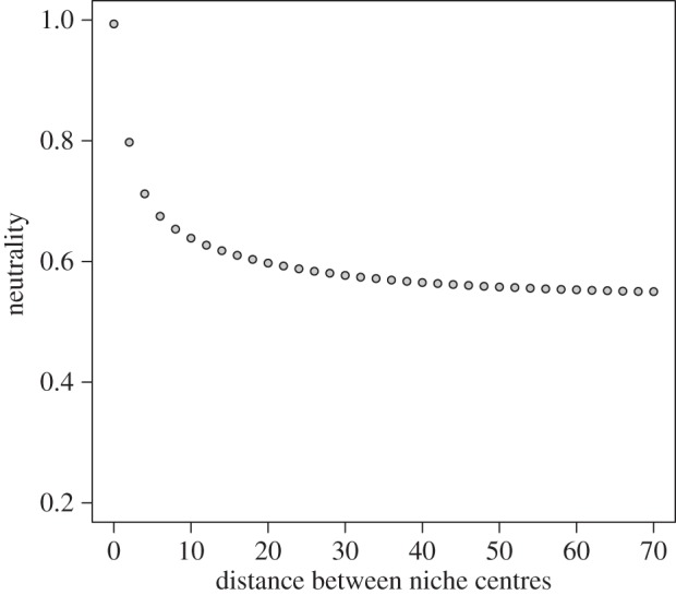
Effects of distance d between niche optimum values on the level of neutrality in a two-species simulation experiment. Species niche breadths (σ parameter in equation (2.2)) were held constant at a value of 5.

(c). Landscape generation and environmental heterogeneity

Landscape heterogeneity consists of two components: spatial configuration and abundance distribution [21]. Here, we generated sets of simulated landscapes, altering each component separately. We generated the model landscape consisting of 128 × 128 cells using a fractal algorithm, the diamond-square method [34]. The landscape was built as a torus to eliminate edge effects. Spatial configuration depends on the single algorithm parameter, H, which represents the level of aggregation in the resulting landscape. Low H-values generate fine-grained landscapes, which resemble random noise; high H-values generate aggregated landscape patterns. In order to vary abundance distribution among landscapes with a given aggregation level, we generated different abundance distributions posteriori, by performing image-processing histogram operations on the distribution of E values. To create intermediate abundance distributions (from very narrow to very broad), we employed histogram stretching techniques. These manipulations retained the spatial configuration of the landscapes and altered only the abundance distribution of E by increasing (or decreasing) the contrast among landscape cells (figure 2). To quantify the degree of abundance distribution in a simulated landscape, we calculated the mean standard deviation of cell values for each landscape map used in our analysis.

Figure 2.

Landscapes with different combinations of two components of environmental heterogeneity: spatial configuration of resources (vertical axis) and abundance distribution of resources (horizontal axis). (Online version in colour.)

(d). Model experiments

To test our hypotheses about the effects of environmental heterogeneity on the location of communities along the niche neutrality continuum, we conducted model simulations with various landscape configurations and relative abundances of E. In addition, we altered the size of the dispersal kernels and the ratio of propagule arrival from the regional species pool (m). We simulated community dynamics for the following parameter ranges: 20 spatial configurations of E, from H = 0.1 to H = 2; four abundance distributions of E, from standard deviation of approximately 7 (very narrow distribution around a mean of E = 50; hereafter referred as ‘very narrow’), through standard deviations of approximately 11 and approximately 16 (hereafter referred as ‘narrow’ and ‘regular’ distributions, respectively), to a uniform abundance distribution of E; 250 species; dispersal kernel sizes of 3, 5, 7, 9 and 11 cells at each dimension; and proportion of propagule arrival from the regional species pool of 0.1 and 0.5. Each simulation with a unique parameter combination was repeated 500 times to account for the inherent stochasticity in model behaviour.

3. Results

Both components of environmental heterogeneity, the spatial configuration and the abundance distribution of the environmental variable (E), had a significant effect on the degree of community neutrality. The shape of the relationship between neutrality and spatial configuration was affected by the abundance distribution of the environmental variable in a unique way, coupled with the size of the dispersal kernel (figure 3). At the smallest dispersal kernel size, neutrality always decreased with increasing H, even at very narrow abundance distributions (figure 3a). By contrast, when species had intermediate (7 × 7 cells; figure 3b) and large dispersal kernels (11 × 11 cells; figure 3c), landscapes closer to uniform abundance distributions of resources exhibited a threshold effect, where at low aggregation levels (and regardless of the size of the dispersal kernel), neutrality was either constant or increased with aggregation levels. Once aggregation increased above a certain threshold, there was a sharp decrease in neutrality with any further increase in aggregation levels. These patterns were most pronounced in the case of the largest dispersal kernels (i.e. 11 × 11 cells, figure 3c). In landscapes with narrower abundance distributions (small standard deviations of E; bottom two curves in figure 3), the relationship between H and neutrality depended on the size of the dispersal kernel. Neutrality was not related to H at very narrow abundance distributions when the size of the dispersal kernel was 7×7 cells (figure 3b). When the dispersal kernel was 11 × 11 cells, neutrality had a weak positive relationship with H (figure 3c). In general, though, narrower resource abundance distributions yielded lower neutrality levels compared with wider resource abundance distributions, and these results were consistent across resource aggregation levels and dispersal kernel sizes. We observed similar relationships between neutrality, resource aggregation and resource abundance distributions when we increased the proportion m of propagule arrival from the regional species pool from 0.1 to 0.5. Yet the overall level of neutrality was slightly higher at m = 0.5 for any given combination of heterogeneity parameters.

Figure 3.

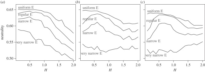
Effects of spatial configuration of resources (H) on neutrality at different resource abundance distribution levels. Panels depict different dispersal kernels: (a) 3 × 3 cells; (b) 7 × 7 cells; and (c) 11 × 11 cells. Different resource abundance distribution levels are depicted by different curves, with the type of the distribution labelled.

The relationship between neutrality and the size of the dispersal kernel depended on the level of resource aggregation, as well as the abundance distribution of resources (figure 4). At high resource aggregation levels, neutrality increased asymptotically with increasing sizes of dispersal kernels. These results were consistent in both narrow and regular resource abundance distributions (figure 4a,b, respectively). By contrast, at low resource aggregation levels, the relationship between neutrality and size of the dispersal kernel was either flat or negative. These results were consistent across all resource abundance distribution levels.

Figure 4.

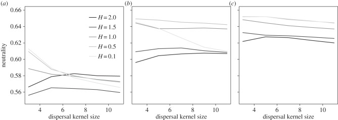
Effects of the size of the dispersal kernel on community neutrality, at different resource aggregation levels (H, depicted by curves with different grey shades). Each panel denotes different resource abundance distributions: (a) narrow, (b) regular and (c) uniform.

4. Discussion

Here, we report on the first indication that environmental heterogeneity, manifested by the spatial configuration of resources as well as their spatially implicit abundance distribution, affects the location of modelled communities along the hypothesized niche–neutrality continuum. We show that landscape heterogeneity affects the degree of community neutrality via its interaction with dispersal processes. The likelihood of propagule establishment depends on its ability to arrive in a favourable site, while the spatial distribution of such favourable sites relative to propagule sources is a direct function of environmental heterogeneity.

We found that even when species have different niche requirements, neutral patterns can emerge [9]. Our results put in context the findings of a recent empirical study [35] that revealed increased niche differentiation among species in more heterogeneous environments. We suggest that, although environmental heterogeneity may promote niche differentiation among species, it can also lead to community-scale neutral dynamics via processes such as mass effects [36]. This is because species establishment in gaps (and subsequently community composition) is the outcome of two processes: stochastic dispersal and deterministic niche differentiation. In classic niche systems, the most suitable propagule will establish in a gap. Yet, in our simulations, when the propagule abundance of a less suitable species was much higher than that of a suitable species, the factor of relative propagule abundance appeared to take precedence over niche superiority, leading to more neutral system dynamics. This mass effect is related to the use of the lottery model for competition for space as a means to determine establishment in gaps [4,23]. The relative effect of both niche differentiation and dispersal on the community's location along the niche–neutrality continuum depends on the environmental heterogeneity of resources surrounding the gap where establishment of a new individual is about to occur, coupled with the characteristics of species' dispersal kernels.

We found that neutrality decreased with increasing resource aggregation at wide resource abundance distributions, but was mostly unrelated to resource aggregation at narrow resource abundance distributions. We explain this relationship in the following way. In landscapes with nearly uniform abundance distribution of resources, every species has about the same number of sites that are suitable for its establishment. The spatial distribution of resources relative to propagule sources and the size of the dispersal kernel dictate the strength of deterministic succession (which reduces neutrality). When resources are highly aggregated, neighbouring sites are similar, and the most suitable propagules are thus likely to arrive in sites as they are already abundant in neighbouring sites [21]. In such cases, community dynamics follow a more deterministic path and neutrality decreases. By contrast, when resource aggregation is low (and H approaches zero), the propagule pool arriving in an available cell is likely to be more diverse, and therefore the outcome of the establishment dynamics is more stochastic, and neutrality increases. In landscapes with very narrow distributions of resources, most species will be poorly adapted to the environmental conditions in most sites, and the few species that are suitable to the prevailing conditions will dominate the community. In such cases, spatial configuration plays a negligible role in community assembly (i.e. neutrality is independent of resource aggregation; bottom curves in figure 3), because a handful of species will establish in a deterministic manner in the most suitable sites regardless of aggregation levels because there will be sufficient propagules of the most suitable species everywhere. Furthermore, in our model, landscapes with narrow resource abundance distributions can support fewer species than landscapes with uniform resource abundance distribution (i.e. a larger niche space), and therefore the lower neutrality in resource-poor landscapes is also an outcome of the much lower species richness within single cells across multiple model simulations. These results corroborate a previous modelling study [8], which showed that increased species richness (leading to increased niche overlap) indeed leads to an increase in neutrality.

The threshold effect we found in the relationship between neutrality and spatial configuration at low aggregation levels was due to the interaction between fine-scale landscape heterogeneity and the size of the dispersal kernel. In landscapes with low aggregation levels, there is considerable fine-scale variation in resources, even within an area equivalent to the smallest dispersal kernel. Therefore, propagules of multiple species may arrive in a focal cell in nearly even abundances. The resulting large species diversity can mask the niche-based advantage in establishment probability of the species best suited for the cell's conditions and may allow less suited species to persist [37]. By contrast, in highly aggregated landscapes (and after a sufficient period of time), the area around a focal cell may consist of a smaller number of species compared with less aggregated landscapes. Consequently, when dispersal distances are short, community dynamics follow a more deterministic route, as the environmental conditions favour a species that is already dominant in the propagule pool. In our model, species had identical dispersal capabilities. By contrast, dispersal capabilities of real species evolve independently. In spatially autocorrelated (or aggregated) environments, the distance to a suitable habitat is short, and selection favours shorter dispersal distances [38]. However, where environmental heterogeneity increases the chances of propagule arrival into unsuitable habitat (owing to low spatial autocorrelation of resources), the induced costs on dispersing individuals can increase selection pressure against dispersal in general [21,39].

The dual relationships we found between neutrality and the size of the dispersal kernel expand the findings of Gravel et al. [8]. They reported a positive relationship between neutrality and dispersal distances, and suggested that larger dispersal kernels can introduce more species into the propagule pool, which is initially dominated by the locally most suitable species. Consequently, the outcome of the establishment process is more stochastic, and neutrality can increase. Our results were similar, but only in cases of high resource aggregation. The spatial configuration of resources used by Gravel et al. [8] was highly aggregated; hence the agreement with our findings at high resource aggregation levels. However, we also found negative relationships between neutrality and dispersal distances at low resource aggregation levels. To understand this result, we analysed species abundances in pre-establishment propagule pools in cells (i.e. before the lottery process selected a single propagule for establishment). At low resource aggregation levels, cell-specific propagule species evenness was much higher at shorter dispersal distances. By contrast, under highly aggregated resources, we found the opposite pattern (i.e. longer dispersal distances increased the evenness of the propagule species pool in any given cell, since species from more dissimilar sites could arrive in a cell). In both cases, increased evenness in a cell's propagule pool translated to increased evenness across independent model simulations. Therefore, dispersal distance coupled with resource aggregation levels dictated the abundance distributions of species in each cell's propagule pool, and subsequently affected neutrality levels across the entire landscape. The two contrasting relationships between neutrality and dispersal distances arose from this unique interaction.

The great challenge in studying niche–neutrality questions remains the difficulty of measuring neutrality in real communities. This requires information about communities’ composition, structure and, most importantly, spatio-temporal dynamics in relation to the resource space. Models are at present the most reliable tools for studying the niche–neutrality continuum hypothesis. Using a modelling approach, we showed that environmental heterogeneity interacts with species' dispersal characteristics to determine the location of communities along the hypothesized niche–neutrality continuum. Environmental heterogeneity is often overlooked in the niche–neutrality debate, which mostly focuses on intrinsic community properties. Our results highlight the role of the environment in structuring communities, and may lead a step further towards a synthetic understanding of community structure and dynamics.

Funding statement

This study was financially supported by the Israel Science Foundation (grant no. 486-2010) and by a grant from the research authority of Oranim College.

References

- 1.Chase JM. 2003. Community assembly: when should history matter? Oecologia 136, 489–498 (doi:10.1007/s00442-003-1311-7) [DOI] [PubMed] [Google Scholar]
- 2.Götzenberger L, et al. 2011. Ecological assembly rules in plant communities: approaches, patterns and prospects. Biol. Rev. 87, 111–127 (doi:10.1111/j.1469-185X.2011.00187.x) [DOI] [PubMed] [Google Scholar]
- 3.Hutchinson GE. 1953. Homage to Santa Rosalia, or Why are there so many kinds of animals? Am. Nat. 93, 145–159 (doi:10.1086/282070) [Google Scholar]
- 4.Hubbell SP. 2001. A unified theory of biodiversity and biogeography. Princeton, NJ: Princeton University Press [Google Scholar]
- 5.Bell G. 2001. Neutral macroecology. Science 293, 2413–2418 (doi:10.1126/science.293.5539.2413) [DOI] [PubMed] [Google Scholar]
- 6.Purves DW, Pacala SW. 2005. Ecological drift in niche-structured communities: neutral pattern does not imply neutral process. In Biotic interactions in the tropics: their role in the maintenance of species diversity (eds Burslem D, Pinard M, Hartley S.), pp. 107–138 Cambridge, UK: Cambridge University Press [Google Scholar]
- 7.Tilman D. 2004. Niche tradeoffs, neutrality, and community structure: a stochastic theory of resource competition, invasion, and community assembly. Proc. Natl Acad. Sci. USA 101, 10 854–10 861 (doi:10.1073/pnas.0403458101) [DOI] [PMC free article] [PubMed] [Google Scholar]
- 8.Gravel D, Canham CD, Beaudet M, Messier C. 2006. Reconciling niche and neutrality: the continuum hypothesis. Ecol. Lett. 9, 399–409 (doi:10.1111/j.1461-0248.2006.00884.x) [DOI] [PubMed] [Google Scholar]
- 9.Holt RD. 2006. Emergent neutrality. Trends Ecol. Evol. 21, 531–533 (doi:10.1016/j.tree.2006.08.003) [DOI] [PubMed] [Google Scholar]
- 10.Adler PB, HilleRisLambers J, Levine JM. 2007. A niche for neutrality. Ecol. Lett. 10, 95–104 (doi:10.1111/j.1461-0248.2006.00996.x) [DOI] [PubMed] [Google Scholar]
- 11.Chisholm RA, Pacala SW. 2011. Theory predicts a rapid transition from niche-structured to neutral biodiversity patterns across a speciation-rate gradient. Theor. Ecol. 4, 195–200 (doi:10.1007/s12080-011-0113-5) [Google Scholar]
- 12.McGill BJ, Maurer BA, Weiser MD. 2006. Empirical evaluation of neutral theory. Ecology 87, 1411–1423 (doi:10.1890/0012-9658(2006)87[1411:EEONT]2.0.CO;2) [DOI] [PubMed] [Google Scholar]
- 13.Chisholm RA, Pacala SW. 2010. Niche and neutral models predict asymptotically equivalent species abundance distributions in high-diversity ecological communities. Proc. Natl Acad. Sci. USA 107, 15 821–15 825 (doi:10.1073/pnas.1009387107) [DOI] [PMC free article] [PubMed] [Google Scholar]
- 14.Gotelli NJ, McGill BJ. 2006. Null versus neutral models: what's the difference? Ecography 29, 793–800 (doi:10.1111/j.2006.0906-7590.04714.x) [Google Scholar]
- 15.Diamond J. 1975. Assembly of species communities. In Ecology and evolution of communities (eds Cody ML, Diamond JM.), pp. 342–444 Cambridge, MA: Harvard University Press [Google Scholar]
- 16.Bell G. 2005. The co-distribution of species in relation to the neutral theory of community ecology. Ecology 86, 1757–1770 (doi:10.1890/04-1028) [Google Scholar]
- 17.Kadmon R, Allouche O. 2007. Integrating the effects of area, isolation, and habitat heterogeneity on species diversity: a unification of island biogeography and niche theory. Am. Nat. 170, 443–454 (doi:10.1086/519853) [DOI] [PubMed] [Google Scholar]
- 18.Giller PS. 1984. Community structure and the niche. London, UK: Chapman and Hall [Google Scholar]
- 19.Scheffer M, van Ness EH. 2006. Self-organized similarity, the evolutionary emergence of groups of similar species. Proc. Natl Acad. Sci. USA 103, 6230–6235 (doi:10.1073/pnas.0508024103) [DOI] [PMC free article] [PubMed] [Google Scholar]
- 20.Kolasa J, Rollo CD. 1991. The heterogeneity of heterogeneity: a glossary. In Ecological heterogeneity (eds Kolasa J, Pickett STA.), pp. 1–23 New York, NY: Springer [Google Scholar]
- 21.Büchi L, Vuilleumier S. 2012. Dispersal strategies, few dominating or many coexisting: The effect of environmental spatial structure and multiple sources of mortality. PLoS ONE 7, e34733 (doi:10.1371/journal.pone.0034733) [DOI] [PMC free article] [PubMed] [Google Scholar]
- 22.Schachak M, Brand S. 1991. Relations among spatiotemporal heterogeneity, population abundance and variability in a desert. In Ecological heterogeneity (eds Kolasa J, Pickett STA.), pp. 202–223 New York, NY: Springer [Google Scholar]
- 23.Chesson PL, Warner R. 1981. Environmental variability promotes coexistence in lottery competitive systems. Am. Nat. 117, 923–943 (doi:10.1086/283778) [Google Scholar]
- 24.Snyder RE, Chesson PL. 2004. How the spatial scales of dispersal, competition, and environmental heterogeneity interact to affect coexistence. Am. Nat. 164, 633–650 (doi:10.1086/424969) [DOI] [PubMed] [Google Scholar]
- 25.Gabay O, Perevolotsky A, Bar Massada A, Carmel Y, Schachak M. 2011. Differential effects of goat browsing on herbaceous plant community in a two-phase mosaic. Plant Ecol. 212, 1643–1653 (doi:10.1007/s11258-011-9937-8) [Google Scholar]
- 26.Bar Massada A, Wood EM, Pidgeon AM, Radeloff VC. 2012. Complex effects of scale on the relationships of landscape pattern versus avian species richness and community structure in a woodland savanna mosaic. Ecography 35, 393–411 (doi:10.1111/j.1600-0587.2011.07097.x) [Google Scholar]
- 27.Levin SA, Cohen D, Hastings A. 1984. Dispersal strategies in patchy environments. Theor. Popul. Biol. 26, 165–191 (doi:10.1016/0040-5809(84)90028-5) [Google Scholar]
- 28.McPeek MA, Holt RD. 1992. The evolution of dispersal in spatially and temporally varying environments. Am. Nat. 140, 1010–1027 (doi:10.1086/285453) [Google Scholar]
- 29.Troupin D, Nathan R, Vendramin GG. 2006. Analysis of spatial genetic structure in an expanding Pinus halepensis population reveals development of fine-scale genetic clustering over time. Mol. Ecol. 15, 3617–3630 (doi:10.1111/j.1365-294X.2006.03047.x) [DOI] [PubMed] [Google Scholar]
- 30.R Development Core Team. 2012. R: a language and environment for statistical computing. Vienna, Austria: R Foundation for Statistical Computing [Google Scholar]
- 31.Chisholm RA, Lichstein JW. 2009. Linking dispersal, immigration and scale in the neutral theory of biodiversity. Ecol. Lett. 12, 1385–1393 (doi:10.1111/j.1461-0248.2009.01389.x) [DOI] [PubMed] [Google Scholar]
- 32.Etienne RS. 2005. A new sampling formula for neutral biodiversity. Ecol. Lett. 8, 253–260 (doi:10.1111/j.1461-0248.2004.00717.x) [Google Scholar]
- 33.Volkov I, Banavar JR, Hubbell SP, Maritan A. 2007. Patterns of relative species abundance in rainforests and coral reefs. Nature 450, 45–49 (doi:10.1038/nature06197) [DOI] [PubMed] [Google Scholar]
- 34.Fournier A, Fussell D, Carpenter L. 1982. Computer rendering of stochastic models. Commun. ACM 25, 371–384 (doi:10.1145/358523.358553) [Google Scholar]
- 35.Brown C, et al. 2013. Multispecies coexistence of trees in tropical forests: spatial signals of topographic niche differentiation increase with environmental heterogeneity. Proc. R. Soc. B 280, 20130502 (doi:10.1098/rspb.2013.0502) [DOI] [PMC free article] [PubMed] [Google Scholar]
- 36.Shmida A, Wilson MV. 1985. Biological determinants of species diversity. J. Biogeogr. 12, 1–20 (doi:10.2307/2845026) [Google Scholar]
- 37.Levene H. 1953. Genetic equilibrium when more than one ecological niche is available. Am. Nat. 87, 331–333 (doi:10.1086/281792) [Google Scholar]
- 38.Travis JMJ, Dytham C. 1999. Habitat persistence, habitat availability and the evolution of dispersal. Proc. R. Soc. Lond. B 266, 723–728 (doi:10.1098/rspb.1999.0696) [Google Scholar]
- 39.Hastings A. 1983. Can spatial variation alone lead to selection for dispersal? Theor. Popul. Biol. 24, 244–251 (doi:10.1016/0040-5809(83)90027-8) [Google Scholar]