The Dropout Learning Algorithm

Abstract

Dropout is a recently introduced algorithm for training neural network by randomly dropping units during training to prevent their co-adaptation. A mathematical analysis of some of the static and dynamic properties of dropout is provided using Bernoulli gating variables, general enough to accommodate dropout on units or connections, and with variable rates. The framework allows a complete analysis of the ensemble averaging properties of dropout in linear networks, which is useful to understand the non-linear case. The ensemble averaging properties of dropout in non-linear logistic networks result from three fundamental equations: (1) the approximation of the expectations of logistic functions by normalized geometric means, for which bounds and estimates are derived; (2) the algebraic equality between normalized geometric means of logistic functions with the logistic of the means, which mathematically characterizes logistic functions; and (3) the linearity of the means with respect to sums, as well as products of independent variables. The results are also extended to other classes of transfer functions, including rectified linear functions. Approximation errors tend to cancel each other and do not accumulate. Dropout can also be connected to stochastic neurons and used to predict firing rates, and to backpropagation by viewing the backward propagation as ensemble averaging in a dropout linear network. Moreover, the convergence properties of dropout can be understood in terms of stochastic gradient descent. Finally, for the regularization properties of dropout, the expectation of the dropout gradient is the gradient of the corresponding approximation ensemble, regularized by an adaptive weight decay term with a propensity for self-consistent variance minimization and sparse representations.

1 Introduction

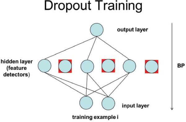
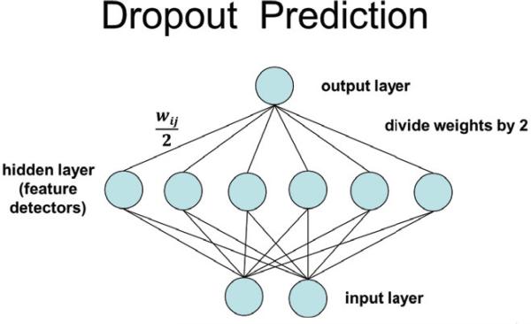
Dropout is a recently introduced algorithm for training neural networks [27]. In its simplest form, on each presentation of each training example, each feature detector unit is deleted randomly with probability q = 1 – p = 0.5. The remaining weights are trained by backpropagation [40]. The procedure is repeated for each example and each training epoch, sharing the weights at each iteration (Figure 1.1). After the training phase is completed, predictions are produced by halving all the weights (Figure 1.2). The dropout procedure can also be applied to the input layer by randomly deleting some of the input-vector components–typically an input component is deleted with a smaller probability (i.e. q = 0.2).

Figure 1.1.

Dropout training in a simple network. For each training example, feature detector units are dropped with probability 0.5. The weights are trained by backpropagation (BP) and shared with all the other examples.

Figure 1.2.

Dropout prediction in a simple network. At prediction time, all the weights from the feature detectors to the output units are halved.

The motivation and intuition behind the algorithm is to prevent overfitting associated with the co-adaptation of feature detectors. By randomly dropping out neurons, the procedure prevents any neuron from relying excessively on the output of any other neuron, forcing it instead to rely on the population behavior of its inputs. It can be viewed as an extreme form of bagging [17], or as a generalization of naive Bayes [23], as well as denoising autoencoders [42]. Dropout has been reported to yield remarkable improvements on several difficult problems, for instance in speech and image recognition, using well known benchmark datasets, such as MNIST, TIMIT, CIFAR-10, and ImageNet [27].

In [27], it is noted that for a single unit dropout performs a kind of “geometric” ensemble averaging and this property is conjectured to extend somehow to deep multilayer neural networks. Thus dropout is an intriguing new algorithm for shallow and deep learning, which seems to be effective, but comes with little formal understanding and raises several interesting questions. For instance:

1. What kind of model averaging is dropout implementing, exactly or in approximation, when applied to multiple layers?

2. How crucial are its parameters? For instance, is q = 0.5 necessary and what happens when other values are used? What happens when other transfer functions are used?

3. What are the effects of different deletion randomization procedures, or different values of q for different layers? What happens if dropout is applied to connections rather than units?

4. What are precisely the regularization and averaging properties of dropout?

5. What are the convergence properties of dropout?

To answer these questions, it is useful to distinguish the static and dynamic aspects of dropout. By static we refer to properties of the network for a fixed set of weights, and by dynamic to properties related to the temporal learning process. We begin by focusing on static properties, in particular on understanding what kind of model averaging is implemented by rules like ”halving all the weights”. To some extent this question can be asked for any set of weights, regardless of the learning stage or procedure. Furthermore, it is useful to first study the effects of droupout in simple networks, in particular in linear networks. As is often the case [8, 9], understanding dropout in linear networks is essential for understanding dropout in non-linear networks.

Related Work. Here we point out a few connections between dropout and previous literature, without any attempt at being exhaustive, since this would require a review paper by itself. First of all, dropout is a randomization algorithm and as such it is connected to the vast literature in computer science and mathematics, sometimes a few centuries old, on the use of randomness to derive new algorithms, improve existing ones, or prove interesting mathematical results (e.g. [22, 3, 33]). Second, and more specifically, the idea of injecting randomness into a neural network is hardly new. A simple Google search yields dozen of references, many dating back to the 1980s (e.g. [24, 25, 30, 34, 12, 6, 37]). In these references, noise is typically injected either in the input data or in the synaptic weights to increase robustness or regularize the network in an empirical way. Injecting noise into the data is precisely the idea behind denoising autoencoders [42], perhaps the closest predecessor to dropout, as well as more recent variations, such as the marginalized-corrupted-features learning approach described in [29]. Finally, since the posting of [27], three articles with dropout in their title were presented at the NIPS 2013 conference: a training method based on overlaying a dropout binary belief network on top of a neural network [7]; an analysis of the adaptive regularizing properties of dropout in the shallow linear case suggesting some possible improvements [43]; and a subset of the averaging and regularization properties of dropout described primarily in Sections 8 and 11 of this article [10].

2 Dropout for Shallow Linear Networks

In order to compute expectations, we must associate well defined random variables with unit activities or connection weights when these are dropped. Here and everywhere else we will consider that a unit activity or connection is set to 0 when the unit or connection is dropped.

2.1 Dropout for a Single Linear Unit (Combinatorial Approach)

We begin by considering a single linear unit computing a weighted sum of n inputs of the form

$$S=S\left(I\right)=\sum _{i=1}^n{w}_i{I}_i$$ (1)

where I = (I₁, . . . , I_n) is the input vector. If we delete inputs with a uniform distribution over all possible subsets of inputs, or equivalently with a probability q = 0.5 of deletion, then there are 2ⁿ possible networks, including the empty network. For a fixed I, the average output over all these networks can be written as:

$$E\left(s\right)=\frac{1}{2^n}\sum _{\mathcal{N}}S(\mathcal{N},I)$$ (2)

where $\mathcal{N}$ is used to index all possible sub-networks, i.e. all possible edge deletions. Note that in this simple case, deletion of input units or of edges are the same thing. The sum above can be expanded using networks of size 0, 1, 2, . . . n in the form

$$E\left(S\right)=\frac{1}{2^n}\left[0+\left(\sum _{i=1}^n{w}_i{I}_i\right)+(\sum _{1\le i<j\le n}{w}_i{I}_i+w_j{I}_j)+\dots \right]$$ (3)

In this expansion, the term w_iI_i occurs

$$1+\left(\begin{array}{c}\hfill n-1\hfill \\ \hfill 1\hfill \end{array}\right)+\left(\begin{array}{c}\hfill n-1\hfill \\ \hfill 2\hfill \end{array}\right)+\dots \left(\begin{array}{c}\hfill n-1\hfill \\ \hfill n-1\hfill \end{array}\right)=2^{n-1}$$ (4)

times. So finally the average output is

$$E\left(S\right)=\frac{2^{n-1}}{2^n}\left(\sum _{i=1}^n{w}_i{I}_i\right)=\sum _{i=1}^n\frac{w_i}{2}{I}_i$$ (5)

Thus in the case of a single linear unit, for any fixed input I the output obtained by halving all the weights is equal to the arithmetic mean of the outputs produced by all the possible sub-networks. This combinatorial approach can be applied to other cases (e.g. p ≠ 0.5) but it is much easier to work directly with a probabilistic approach.

2.2 Dropout for a Single Linear Unit (Probabilistic Approach)

Here we simply consider that the output is a random variable of the form

$$S=\sum _{i=1}^n{w}_i{\delta }_i{I}_i$$ (6)

where δ_i is a Bernoulli selector random variable, which deletes the weight w_i (equivalently the input I_i) with probability P(δ_i = 0) = q_i. The Bernoulli random variables are assumed to be independent of each other (in fact pairwise independence, as opposed to global independence, is sufficient for all the results to be presented here). Thus P(δ_i = 1) = 1 – q_i = p_i. Using the linearity of the expectation we have immediately

$$E\left(S\right)=\sum _{i=1}^n{w}_{i}E\left({\delta }_i\right)I_i=\sum _{i=1}^n{w}_i{p}_i{I}_i$$ (7)

This formula allows one to handle different p_i for each connection, as well as values of p_i that deviate from 0.5. If all the connections are associated with independent but identical Bernoulli selector random variables with p_i = p, then

$$E\left(S\right)\sum _{i=1}^n{w}_{i}E\left(\delta \right)I_i=\sum _{i=1}^n{w}_{i}p{I}_i$$ (8)

Thus note, for instance, that if the inputs are deleted with probability 0.2 then the expected output is given by 0.8 ${\sum }_i{w}_i{I}_i$. Thus the weights must be multiplied by 0.8. The key property behind Equation 8 is the linearity of the expectation with respect to sums and multiplications by scalar values, and more generally for what follows the linearity of the expectation with respect to the product of independent random variables. Note also that the same approach could be applied for estimating expectations over the input variables, i.e. over training examples, or both (training examples and subnetworks). This remains true even when the distribution over examples is not uniform.

If the unit has a fixed bias b (affine unit), the random output variable has the form

$$S=\sum _{i=1}^n{w}_i{\delta }_i{I}_i+b{\delta }_b$$ (9)

The case where the bias is always present, i.e. when δ_b = 1 always, is just a special case. And again, by linearity of the expectation

$$E\left(S\right)=\sum _{i=1}^n{w}_i{p}_i{I}_i+b{p}_b$$ (10)

where P(δ_b = 1) = p_b. Under the natural assumption that the Bernoulli random variables are independent of each other, the variance is linear with respect to the sum and can easily be calculated in all the previous cases. For instance, starting from the most general case of Equation 9 we have

$$Var\left(S\right)=\sum _{i=1}^n{w}_i^{2}Var\left({\delta }_i\right)I_i^2+b^{2}Var\left({\delta }_b\right)=\sum _{i=1}^n{w}_i^2{p}_i{q}_i{I}_i^2+b^2{p}_b{q}_b$$ (11)

with q_i = 1 – p_i. S can be viewed as a weighted sum of independent Bernoulli random variables, which can be approximated by a Gaussian random variable under reasonable assumptions.

2.3 Dropout for a Single Layer of Linear Units

We now consider a single linear layer with k output units

$$S_i\left(I\right)=\sum _{j=1}^n{w}_{ij}{I}_j\text{for}i=1,\dots ,k$$ (12)

In this case, dropout applied to input units is slightly different from dropout applied to the connections. Dropout applied to the input units leads to the random variables

$$S_i\left(I\right)=\sum _{j=1}^n{w}_{ij}{\delta }_j{I}_j\text{for}i=1,\dots ,k$$ (13)

whereas dropout applied to the connections leads to the random variables

$$S_i\left(I\right)=\sum _{j=1}^n{\delta }_{ij}{w}_{ij}{I}_j\text{for}i=1,\dots ,k$$ (14)

In either case, the expectations, variances, and covariances can easily be computed using the linearity of the expectation and the independence assumption. when dropout is applied to the input units, we get:

$$E\left(S_i\right)=\sum _{j=1}^n{w}_{ij}{p}_j{I}_j\text{for}i=1,\dots ,k$$ (15)

$$Var\left(S_i\right)=\sum _{j=1}^n{w}_{ij}^2{p}_j{q}_j{I}_j^2\text{for}i=1,\dots ,k$$ (16)

$$Cov(S_i,S_l)=\sum _{j=1}^n{w}_{ij}{w}_{lj}{p}_j{q}_j{I}_j^2\text{for}1\le i<l\le k$$ (17)

When dropout is applied to the connections, we get:

$$E\left(S_i\right)=\sum _{j=1}^n{w}_{ij}{p}_{ij}{I}_j\text{for}i=1,\dots ,k$$ (18)

$$Var\left(S_i\right)=\sum _{j=1}^n{w}_{ij}^2{p}_{ij}{q}_{ij}{I}_j^2\text{for}i=1,\dots ,k$$ (19)

$$Cov(S_i,S_l)=0\text{for}1\le i<l\le k$$ (20)

Note the difference in covariance between the two models. When dropout is applied to the connections, S_i and S_l are entirely independent.

3 Dropout for Deep Linear Networks

In a general feedforward linear network described by an underlying directed acyclic graph, units can be organized into layers using the shortest path from the input units to the unit under consideration. The activity in unit i of layer h can be expressed as:

$$S_i^h\left(I\right)=\sum _{l<h}\sum _j{w}_{ij}^{hl}{S}_j^l\text{wit}{S}_j^0=I_j$$ (21)

Again, in the general case, dropout applied to the units is slightly different from dropout applied to the connections. Dropout applied to the units leads to the random variables

$$S_i^h=\sum _{l<h}\sum _j{w}_{ij}^{hl}{\delta }_j^l{S}_j^l\text{with}{S}_j^0=I_j$$ (22)

whereas dropout applied to the connections leads to the random variables

$$S_i^h=\sum _{l<h}\sum _j{\delta }_{ij}^{hl}{w}_{ij}^{hl}{S}_j^l\text{with}{S}_j^0=I_j$$ (23)

When dropout is applied to the units, assuming that the dropout process is independent of the unit activities or the weights, we get:

$$E\left(S_i^h\right)=\sum _{l<h}\sum _j{w}_{ij}^{hl}{p}_j^{l}E\left(S_j^l\right)\text{for}h>0$$ (24)

with $E\left(S_j^0\right)=I_j$ in the input layer. This formula can be applied recursively across the entire network, starting from the input layer. Note that the recursion of Equation 24 is formally identical to the recursion of backpropagation suggesting the use of dropout during the backward pass. This point is elaborated further at the end of Section 10. Note also that although the expectation $E\left(S_i^h\right)$ is taken over all possible subnetworks of the original network, only the Bernoulli gating variables in the previous layers (l < h) matter. Therefore it coincides also with the expectation taken over only all the induced subnetworks of node i(comprising only nodes that are ancestors of node i).

Remarkably, using these expectations, all the covariances can also be computed recursively from the input layer to the output layer, by writing $Cov(S_i^h,S_{i^{\prime }}^{h^{\prime }})=E\left(S_i^h{S}_{i^{\prime }}^{h^{\prime }}\right)-E\left(S_i^h\right)E\left(S_{i^{\prime }}^{h^{\prime }}\right)$ and computing

$$E\left(S_i^h{S}_{i^{\prime }}^{h^{\prime }}\right)=E\left[\sum _{l<h}\sum _j{w}_{ij}^{hl}{\delta }_j^l{S}_j^l\sum _{l^{\prime }<h^{\prime }}\sum _{j^{\prime }}{w}_{i^{\prime }{j}^{\prime }}^{h^{\prime }{l}^{\prime }}{\delta }_{j^{\prime }}^{l^{\prime }}{S}_{j^{\prime }}^{l^{\prime }}\right]=\sum _{l<h}\sum _{l^{\prime }<h^{\prime }}\sum _j\sum _{j^{\prime }}{w}_{ij}^{hl}{w}_{i^{\prime }{j}^{\prime }}^{h^{\prime }{l}^{\prime }}E\left({\delta }_j^l{\delta }_{j^{\prime }}^{l^{\prime }}\right)E\left(S_j^l{S}_{j^{\prime }}^{l^{\prime }}\right)$$ (25)

under the usual assumption that ${\delta }_j^l{\delta }_{j^{\prime }}^{l^{\prime }}$ of is independent of $S_j^l{S}_{j^{\prime }}^{l^{\prime }}$. Furthermore, under the usual assumption that ${\delta }_j^l$ and ${\delta }_{j^{\prime }}^{l^{\prime }}$ are independent when l ≠ l′ or j ≠ j′, we have in this case $E\left({\delta }_j^l{\delta }_{j^{\prime }}^{l^{\prime }}\right)=p_j^l{p}_{j^{\prime }}^{l^{\prime }}$, with furthermore $E\left({\delta }_j^l{\delta }_j^l\right)=p_j^l$. Thus in short under the usual independence assumptions, $E\left(S_i^h{S}_{i^{\prime }}^{h^{\prime }}\right)$ can be computed recursively from the values of $E\left(S_j^l{S}_{j^{\prime }}^{l^{\prime }}\right)$ in lower layers, with the boundary conditions $E\left(I_i{I}_j\right)=I_i{I}_j$ for a fixed input vector (layer 0). The recursion proceeds layer by layer, from the input to the output layer. When a new layer is reached, the covariances to all the previously visited layers must be computed, as well as all the intralayer covariances.

When dropout is applied to the connections, under similar independence assumptions, we get:

$$E\left(S_i^h\right)=\sum _{l<h}\sum _j{p}_{ij}^{hl}{w}_{ij}^{hl}E\left(S_j^l\right)\text{for}h>0$$ (26)

with $E\left(S_j^0\right)=I_j$ in the input layer. This formula can be applied recursively across the entire network. Note again that although the expectation $E\left(S_i^h\right)$ is taken over all possible subnetworks of the original network, only the Bernoulli gating variables in the previous layers (l < h) matter. Therefore it is also the expectation taken over only all the induced subnetworks of node i(corresponding to all the ancestors of node i). Furthermore, using these expectations, all the covariances can also be computed recursively from the input layer to the output layer using a similar analysis to the one given above for the case of dropout applied to the units of a general linear network.

In summary, for linear feedforward networks the static properties of dropout applied to the units or the connections using Bernoulli gating variables that are independent of the weights, of the activities, and of each other (but not necessarily identically distributed) can be fully understood. For any input, the expectation of the outputs over all possible networks induced by the Bernoulli gating variables is computed using the recurrence equations 24 and 26, by simple feedforward propagation in the same network where each weight is multiplied by the appropriate probability associated with the corresponding Bernoulli gating variable. The variances and covariances can also be computed recursively in a similar way.

4 Dropout for Shallow Neural Networks

We now consider dropout in non-linear networks that are shallow, in fact with a single layer of weights.

4.1 Dropout for a Single Non-Linear Unit (Logistic)

Here we consider that the output of a single unit with total linear input S is given by the logistic sigmoidal function

$$O=\sigma \left(S\right)=\frac{1}{1+c{e}^{-\lambda S}}$$ (27)

Here and everywhere else, we must have c ≥ 0 There are 2ⁿ possible sub-networks indexed by $\mathcal{N}$ and, for a fixed input I, each sub-network produces a linear value $S(\mathcal{N},I)$ and a final output value $O_{\mathcal{N}}=\sigma \left(\mathcal{N}\right)=\sigma \left(S(\mathcal{N},I)\right)$. Since I is fixed, we omit the dependence on I in all the following calculations. In the uniform case, the geometric mean of the outputs is given by

$$G=\prod _{\mathcal{N}}{O}_{\mathcal{N}}^{1∕2^n}$$ (28)

Likewise, the geometric mean of the complementary outputs $(1-O_{\mathcal{N}})$ is given by

$$G^{\prime }=\prod _{\mathcal{N}}{(1-O_{\mathcal{N}})}^{1∕2^n}$$ (29)

The normalized geometric mean (NGM) is defined by

$$NGM=\frac{G}{G+G^{\prime }}$$ (30)

The NGM of the outputs is given by

$$NGM\left(O\left(\mathcal{N}\right)\right)=\frac{{\left[{\prod }_{\mathcal{N}}\sigma \left(S\left(\mathcal{N}\right)\right)\right]}^{1∕2^n}}{{\left[{\prod }_{\mathcal{N}}\sigma \left(S\left(\mathcal{N}\right)\right)\right]}^{1∕2^n}+{\left[{\prod }_{\mathcal{N}}(1-\sigma \left(S\left(\mathcal{N}\right)\right))\right]}^{1∕2^n}}=\frac{1}{1+{\left[{\prod }_{\mathcal{N}}\frac{1-\sigma \left(S\left(\mathcal{N}\right)\right)}{\sigma (S\left(\mathcal{N}\right)}\right]}^{1∕2^n}}$$ (31)

Now for the logistic function σ, we have

$$\frac{1-\sigma \left(x\right)}{\sigma \left(x\right)}=c{e}^{-\lambda x}$$ (32)

Applying this identity to Equation 31 yields

$$NGM\left(O\left(\mathcal{N}\right)\right)=\frac{1}{1+{\left[{\prod }_{\mathcal{N}}c{e}^{-\lambda S\left(\mathcal{N}\right)}\right]}^{1∕2^n}}=\frac{1}{1+c\left[e^{-\lambda {\sum }_{\mathcal{N}}S\left(\mathcal{N}\right)∕2^n}\right]}=\sigma \left(E\left(S\right)\right)$$ (33)

where here $E\left(S\right)={\sum }_{\mathcal{N}}S\left(\mathcal{N}\right)∕2^n$. Or, in more compact form,

$$NGM\left(\sigma \left(S\right)\right)=\sigma \left(E\left(S\right)\right)$$ (34)

Thus with a uniform distribution over all possible sub-networks $\mathcal{N}$, equivalent to having i.i.d. input unit selector variables δ = δ_i with probability p_i = 0.5, the NGM is simply obtained by keeping the same overall network but dividing all the weights by two and applying σ to the expectation $E\left(S\right)={\sum }_{i=1}^n\frac{w_i}{2}{I}_i$.

It is essential to observe that this result remains true in the case of a non-uniform distribution over the subnetworks $\mathcal{N}$, such as the distribution generated by Bernoulli gating variables that are not identically distributed, or with p ≠ 0.5. For this we consider a general distribution $P\left(\mathcal{N}\right)$. This is of course even more general than assuming the P is the product of n independent Bernoulli selector variables. In this case, the weighted geometric means are defined by:

$$G=\prod _{\mathcal{N}}{O}_{\mathcal{N}}^{P\left(\mathcal{N}\right)}$$ (35)

and

$$G^{\prime }=\prod _{\mathcal{N}}{(1-O_{\mathcal{N}})}^{P\left(\mathcal{N}\right)}$$ (36)

and similarly for the normalized weighted geometric mean (NWGM)

$$NWGM=\frac{G}{G+G^{\prime }}$$ (37)

Using the same calculation as above in the uniform case, we can then compute the normalized weighted geometric mean NWGM in the form

$$NWGM\left(O\left(\mathcal{N}\right)\right)=\frac{{\prod }_{\mathcal{N}}\sigma {\left(S\left(\mathcal{N}\right)\right)}^{P\left(\mathcal{N}\right)}}{{\prod }_{\mathcal{N}}\sigma {\left(S\left(\mathcal{N}\right)\right)}^{P\left(\mathcal{N}\right)}+{\prod }_{\mathcal{N}}{(1-\sigma \left(S\left(\mathcal{N}\right)\right))}^{P\left(\mathcal{N}\right)}}$$ (38)

$$NWGM\left(O\left(\mathcal{N}\right)\right)=\frac{1}{1+{\prod }_{\mathcal{N}}{\left(\frac{1-\sigma \left(S\left(\mathcal{N}\right)\right)}{\sigma \left(S\left(\mathcal{N}\right)\right)}\right)}^{P\left(\mathcal{N}\right)}}=\frac{1}{1+c{e}^{-\lambda {\sum }_{\mathcal{N}}P\left(\mathcal{N}\right)S\left(\mathcal{N}\right)}}=\sigma \left(E\left(S\right)\right)$$ (39)

where here $E\left(S\right)={\sum }_{\mathcal{N}}P\left(\mathcal{N}\right)S\left(\mathcal{N}\right)$. Thus in summary with any distribution $P\left(\mathcal{N}\right)$ over all possible sub-networks $\mathcal{N}$, including the case of independent but not identically distributed Ninput unit selector variables δ_i with probability p_i, the NW GM is simply obtained by applying the logistic function to the expectation of the linear input S. In the case of independent but not necessarily identically distributed selector variables δ_i, each with a probability p_i of being equal to one, the expectation of S can be computed simply by keeping the same overall network but multiplying each weight w_i by p_i so that $E\left(S\right)={\sum }_{i=1}^n{p}_i{w}_i{I}_i$.

Note that as in the linear case, this property of logistic units is even more general. That is for any set of S₁, . . . , S_m and any associated probability distribution $P_1,\dots ,P_m({\sum }_{i=1}^m{P}_i=1)$ and associated outputs O₁, . . . , O_m (with O = σ(S)), we have $NWGM\left(O\right)=\sigma \left(E\right)=\sigma \left({\sum }_i{P}_i{S}_i\right)$. Thus the NVGM can be computed over inputs, over inputs and subnetworks, or over other distributions than the one associated with subnetworks, even when the distribution is not uniform. For instance, if we add Gaussian or other noise to the weights, the same formula can be applied. Likewise, we can approximate the average activity of an entire neuronal layer, by applying the logistic function to the average input of the neurons in that layer, as long as all the neurons in the layer use the same logistic function. Note also that the property is true for any c and λ and therefore, using the analyses provided in the next sections, it will be applicable to each of the units, in a network where different units have different values of c and λ. Finally, the property is even more general in the sense that the same calculation as above shows that for any function f

$$NWGM(\sigma \left(f\left(S\right)\right)=\sigma (E\left(f\left(S\right)\right)$$ (40)

and in particular, for any k

$$NWGM\left(\sigma \left(S^k\right)\right)=\sigma \left(E\left(S^k\right)\right)$$ (41)

4.2 Dropout for a Single Layer of Logistic Units

In the case of a single output layer of k logistic functions, the network comoutes k linear sums $S_i={\sum }_{j=1}^n{w}_{ij}{I}_j$ for i = 1, . . . , k and then k outputs of the form

$$O_i={\sigma }_i\left(S_i\right)$$ (42)

The dropout procedure produces a subnetwork $\mathcal{M}=({\mathcal{N}}_1,\dots ,{\mathcal{N}}_k)$ where ${\mathcal{N}}_i$ here represents the corresponding sub-network associated with the i-th output unit. For each i, there are 2ⁿ possible sub-networks for unit i, so there are 2^kn possible subnetworks $\mathcal{M}$. In this case, Equation 39 holds for each unit individually. If dropout uses independent Bernoulli selector variables δ_ij on the edges, or more generally, if the sub-networks $({\mathcal{N}}_1,\dots ,{\mathcal{N}}_k)$ are selected independently of each other, then the covariance between any two output units is 0. If dropout is applied to the input units, then the covariance between two sigmoidal outputs may be small but non-zero.

4.3 Dropout for a Set of Normalized Exponential Units

We now consider the case of one layer of normalized exponential units. In this case, we can think of the network as having k outputs obtained by first computing k linear sums of the form $S_i={\sum }_{j=1}^n{w}_{ij}{I}_j$ for i = 1, . . . , k and then k outputs of the form

$$O_i=\frac{e^{\lambda S_i}}{{\sum }_{j=1}^k{e}^{\lambda S_j}}=\frac{1}{1+\left({\sum }_{j\ne i}{e}^{\lambda S_j}\right)e^{-\lambda S_i}}=$$ (43)

Thus O_i is a logistic output but the coefficients of the logistic function depend on the values of S_j for j ≠ i. The dropout procedure produces a subnetwork $\mathcal{M}=({\mathcal{N}}_1,\dots ,{\mathcal{N}}_k)$ where ${\mathcal{N}}_i$ represents the corresponding sub-network associated with the i-th output unit. For each i, there are 2ⁿ possible subnetworks for unit i, so there are 2^kn possible subnetworks $\mathcal{M}$. We assume first that the distribution $P\left(\mathcal{M}\right)$ is factorial, that is $P\left(\mathcal{M}\right)=P\left({\mathcal{N}}_1\right)\dots P\left({\mathcal{N}}_k\right)$, equivalent to assuming that the subnetworks associated with the individual units are chosen independently of each other. This is the case when using independent Bernoulli selector applied to the connections. The normalized weighted geometric average of output unit i is given by

$$NWGM\left(O_i\right)=\frac{{\prod }_{\mathcal{M}}{\left(\frac{e^{\lambda S_i\left({\mathcal{N}}_i\right)}}{{\sum }_{j=1}^k{e}^{\lambda S_j\left({\mathcal{N}}_j\right)}}\right)}^{P\left(\mathcal{M}\right)}}{{\sum }_{j=1}^k{\prod }_{\mathcal{M}}{\left(\frac{e^{\lambda S_j\left({\mathcal{N}}_l\right)}}{{\sum }_{j=1}^k{e}^{\lambda S_j\left({\mathcal{N}}_j\right)}}\right)}^{P\left(\mathcal{M}\right)}}$$ (44)

Simplifying by the numerator

$$NWGM\left(O_i\right)=\frac{1}{1+{\sum }_{l=1,l\ne i}^k{\prod }_{\mathcal{M}}{\left(\frac{e^{\lambda S_l\left({\mathcal{N}}_l\right)}}{e^{\lambda S_i\left({\mathcal{N}}_i\right)}}\right)}^{P\left(\mathcal{M}\right)}}$$ (45)

Factoring and collecting the exponential terms gives

$$NWGM\left(O_i\right)=\frac{1}{1+e^{-{\sum }_{\mathcal{M}}\lambda P\left(\mathcal{M}\right)S_i\left({\mathcal{N}}_i\right)}{\sum }_{l=1,l\ne i}^k{e}^{{\sum }_{\mathcal{M}}\lambda P\left(\mathcal{M}\right)S_l\left({\mathcal{N}}_i\right)}}$$ (46)

$$NWGM\left(O_i\right)=\frac{1}{1+e^{-\lambda E\left(S_i\right)}{\sum }_{l=1,l\ne i}^k{e}^{\lambda E\left(S_l\right)}}=\frac{e^{\lambda E\left(S_i\right)}}{\sum _{l=1}^k{e}^{\lambda E\left(S_l\right)}}$$ (47)

Thus with any distribution $P\left(\mathcal{N}\right)$ over all possible sub-networks $\mathcal{N}$, including the case of independent but not identically distributed input unit selector variables δ_i with probability p_i, the NW GM of a normalized exponential unit is obtained by applying the normalized exponential to the expectations of the underlying linear sums S_i. In the case of independent but not necessarily identically distributed selector variables δ_i, each with a probability p_i of being equal to one, the expectation of S_i can be computed simply by keeping the same overall network but multiplying each weight w_i by p_i so that $E\left(S_i\right)={\sum }_{j=1}^n{p}_j{w}_i{I}_j$.

5 Dropout for Deep Neural Networks

Finally, we can deal with the most interesting case of deep feedforward networks of sigmoidal units ¹, described by a set of equations of the form

$$O_i^h={\sigma }_i^h\left(S_i^h\right)=\sigma \left(\sum _{l<h}\sum _j{w}_{ij}^{hl}{O}_j^l\right)\text{with}{O}_j^0=I_j$$ (48)

Dropout on the units can be described by

$$O_i^h={\sigma }_i^h\left(S_i^h\right)=\sigma \left(\sum _{l<h}\sum _j{w}_{ij}^{hl}{\delta }_j^l{O}_j^l\right)\text{with}{O}_j^0=I_j$$ (49)

using the selector variables ${\delta }_j^l$ and similarly for dropout on the connections. For each sigmoidal unit

$$NWGM\left(O_i^h\right)=\frac{{\prod }_{\mathcal{N}}{\left(O_i^h\right)}^{P\left(\mathcal{N}\right)}}{{\prod }_{\mathcal{N}}{\left(O_i^h\right)}^{P\left(\mathcal{N}\right)}+{\prod }_{\mathcal{N}}{(1-O_i^h)}^{P\left(\mathcal{N}\right)}}$$ (50)

and the basic idea is to approximate expectations by the corresponding NWGMs, allowing the propagation of the expectation symbols from outside the sigmoid symbols to inside.

$$E\left[\sigma \left(S(\mathcal{N},I)\right)\right]\approx NWGM\left[O(\mathcal{N},I)\right]=\sigma \left(E\left[S(\mathcal{N},I)\right]\right)$$ (51)

More precisely, we have the following recursion:

$$E\left(O_i^h\right)\approx NWGM\left(O_i^h\right)$$ (52)

$$NWGM\left(O_i^h\right)={\sigma }_i^h\left[E\left(S_i^h\right)\right]$$ (53)

$$E\left(S_i^h\right)=\sum _{l<h}\sum _j{w}_{ij}^{hl}{p}_j^{l}E\left(O_j^l\right)$$ (54)

Equations 52, 53, and 54 are the fundamental equations underlying the recursive dropout ensemble approximation in deep neural networks. The only direct approximation in these equations is of course Equation 52 which will be discussed in more depth in Sections 8 and 9. This equation is exact if and only if the numbers $O_i^h$ are identical over all possible subnetworks $\mathcal{N}$. However, even when the numbers $O_i^h$ are not identical, the normalized weighted geometric mean ofteNn provides a good approximation. If the network contains linear units, then Equation 52 is not necessary for those units and their average can be computed exactly. The only fundamental assumption for Equation 54 is independence of the selector variables from the activity of the units or the value of the weights so that the expectation of the product is equal to the product of the expectations. Under the same conditions, the same analysis can be applied to dropout gating variables applied to the connections or, for instance, to Gaussian noise added to the unit activities.

Finally, we measure the consistency $C(O_i^h,I)$ of neuron i in layer h for input I by the variance $Var\left[O_i^h\left(I\right)\right]$) taken over all subnetworks $\mathcal{N}$ and their distribution when the input I is fixed. The larger the variance is, the less consistent the neuron is, and the worse we can expect the approximation in Equation 52 to be. Note that for a random variable O in [0,1] the variance is bound to be small anyway, and cannot exceed 1/4. This is because Var(O) = E(O²) – (E(O))² ≤ E(O) – (E(O))² = E(O)(1 – E(O)) ≤ 1/4. The overall input consistency of such a neuron can be defined as the average of $C(O_i^h,I)$ taken over all training inputs I, and similar definitions can be made for the generalization consistency by averaging $C(O_i^h,I)$ over a generalization set.

Before examining the quality of the approximation in Equation 52, we study the properties of the NWGM for averaging ensembles of predictors, as well as the classes of transfer functions satisfying the key dropout NWGM relation (NWGM(f(x)) = f(E(x))) exactly, or approximately.

6 Ensemble Optimization Properties

The weights of a neural network are typically trained by gradient descent on the error function computed using the outputs and the corresponding targets. The error functions typically used are the squared error in regression and the relative entropy in classification. Considering a single example and a single output O with a target t, these errors functions can be written as:

$$Error(O,t)=\frac{1}{2}{(t-O)}^2\text{and}Error(O,t)=-t\log O-(1-t)\log (1-O)$$ (55)

Extension to multiple outputs, including classification with multiple classes using normalized exponential transfer functions, is immediate. These error terms can be summed over examples or over predictors in the case of an ensemble. Both error functions are convex up (∪) and thus a simple application of Jensen's theorem shows immediately that the error of any ensemble average is less than the average error of the ensemble components. Thus in the case of any ensemble producing outputs O₁, . . . , O_m and any convex error function we have

$$Error(\sum _i{p}_i{O}_i,t)\le \sum _i{p}_{i}Error(O_i,t)\text{or}Error\left(E\right)\le E\left(Error\right)$$ (56)

Note that this is true for any individual example and thus it is also true over any set of examples, even when these are not identically distributed. Equation 56 is the key equation for using ensembles and for averaging them arithmetically.

In the case of dropout with a logistic output unit the previous analyses show that the NWGM is an approximation to E and on this basis alone it is a reasonable way of combining the predictors in the ensemble of all possible subnetworks. However the following stronger result holds. For any convex error function, both the weighted geometric mean WGM and its normalized version NWGM of an ensemble possess the same qualities as the expectation. In other words:

$$Error(\prod _i{O}_i^{p_i},t)\le \sum _i{p}_{i}Error(O_i,t)\text{or}Error\left(WGM\right)\le E\left(Error\right)$$ (57)

$$Error(\frac{{\prod }_i{O}_i^{p_i}}{{\prod }_i{O}_i^{p_i}+{\prod }_i{(1-O_i)}^{p_i}},t)\le \sum _i{p}_{i}Error(O_i,t)\text{or}Error\left(NWGM\right)\le E\left(Error\right)$$ (58)

In short, for any convex error function, the error of the expectation, weighted geometric mean, and normalized weighted geometric mean of an ensemble of predictors is always less than the expected error.

Proof: Recall that if f is convex and g is increasing, then the composition f(g) is convex. This is easily shown by directly applying the definition of convexity (see [39, 16] for additional background on convexity). Equation 57 is obtained by applying Jensen's inequality to the convex function Error(g), where g is the increasing function g(x) = e^x, using the points log O₁, . . . , log O_m. Equation 58 is obtained by applying Jensen's inequality to the convex function Error(g), where g is the increasing function g(x) = e^x/(1 + e^x), using the points log O₁ – log(1 – O₁), . . . , log O_m – log(1 – O_m). The cases where some of the O_i are equal to 0 or 1 can be handled directly, although these are irrelevant for our purposes since the logistic output can never be exactly equal to 0 or 1.

Thus in circumstances where the final output is equal to the weighted mean, weighted geometric mean, or normalized weighted geometric mean of an underlying ensemble, Equations 56, 57, or 58 apply exactly. This is the case, for instance, of linear networks, or non-linear networks where dropout is applied only to the output layer with linear, logistic, or normalized-exponential units.

Since dropout approximates expectations using NWGMs, one may be concerned by the errors introduced by such approximations, especially in a deep architecture when dropout is applied to multiple layers. It is worth noting that the result above can be used at least to “shave off” one layer of approximations by legitimizing the use of NWGMs to combine models in the output layer, instead of the expectation. Similarly, in the case of a regression problem, if the output units are linear then the expectations can be computed exactly at the level of the output layer using the results above on linear networks, thus reducing by one the number of layers where the approximation of expectations by NWGMs must be carried. Finally, as shown below, the expectation, the WGM, and the NWGM are relatively close to each other and thus there is some flexibility, hence some robustness in how predictors are combined in an ensemble, in the sense that combining models with approximations to these quantities may still outperform the expectation of the error of the individual models.

Finally, it must also be pointed out that in the prediction phase once can also use expected values, estimated at some computational cost using Monte Carlo methods, rather than approximate values obtained by forward propagation in the network with modified weights.

7 Dropout Functional Classes and Transfer Functions

7.1 Dropout Functional Classes

Dropout seems to rely on the fundamental property of the logistic sigmoidal function NWGM(σ) = σ(E). Thus it is natural to wonder what is the class of functions f satisfying this property. Here we show that the class of functions f defined on the real line with range in [0, 1] and satisfying

$$\frac{G}{G+G^{\prime }}\left(f\right)=f\left(E\right)$$ (59)

for any set of points and any distribution, consists exactly of the union of all constant functions f(x) = K with 0 ≤ K ≤ 1 and all logistic functions f(x) = 1/(1 + ce^–λx). As a reminder, G denotes the geometric mean and G′ denotes the geometric mean of the complements. Note also that all the constant functions with f(x) = K with 0 ≤ K ≤ 1 can also be viewed as logistic functions by taking λ = 0 and c = (1 – K)/K(K = 0 is a limiting case corresponding to c → ∞).

Proof: To prove this result, note first that the [0, 1] range is required by the definitions of G and G′, since these impose that f(x) and 1 – f(x) be positive. In addition, any function f(x) = K with 0 ≤ K ≤ 1 is in the class and we have shown that the logistic functions satisfy the property. Thus we need only to show these are the only solutions.

By applying Equation 59 to pairs of arguments, for any real numbers u and v with u ≤ v and any real number 0 ≤ p ≤ 1, any function in the class must satisfy:

$$\frac{f{\left(u\right)}^{p}f{\left(v\right)}^{1-p}}{f{\left(u\right)}^{p}f{\left(v\right)}^{1-p}+{(1-f\left(u\right))}^p{(1-f\left(v\right))}^{1-p}}=f(pu+(1-p)v)$$ (60)

Note that if f(u) = f(v) then the function f must be constant over the entire interval [u, v]. Note also that if f(u) = 0 and f(v) > 0 then f = 0 in [u, v). As a result, it is impossible for a non-zero function in the class to satisfy f(u) = 0, f(v₁) > 0, and f(v₂) > 0. Thus if a function f in the class is not constantly equal to 0, then f > 0 everywhere. Similarly (and by symmetry), if a function f in the class is not constantly equal to 1, then f < 1 everywhere.

Consider now a function f in the class, different from the constant 0 or constant 1 function so that 0 < f < 1 everywhere. Equation 60 shows that on any interval [u, v] f is completely defined by at most two parameters f(u) and f(v). On this interval, by letting x = pu + (1 – p)v or equivalently p = (v – x)/(v – u) the function is given by

$$f\left(x\right)=\frac{1}{1+{\left(\frac{1-f\left(u\right)}{f\left(u\right)}\right)}^{\frac{v-x}{v-u}}{\left(\frac{1-f\left(v\right)}{f\left(v\right)}\right)}^{\frac{x-u}{v-u}}}$$ (61)

or

$$f\left(x\right)=\frac{1}{1+c{e}^{-\lambda x}}$$ (62)

with

$$c={\left(\frac{1-f\left(u\right)}{f\left(u\right)}\right)}^{\frac{v}{v-u}}{\left(\frac{1-f\left(v\right)}{f\left(v\right)}\right)}^{\frac{-u}{v-u}}$$ (63)

and

$$\lambda =\frac{1}{v-u}\log \left(\frac{1-f\left(u\right)}{f\left(u\right)}\frac{f\left(v\right)}{1-f\left(v\right)}\right)$$ (64)

Note that a particular simple parameterization is given in terms of

$$f\left(0\right)=\frac{1}{1+c}\text{and}f\left(x\right)=\frac{1}{2}\text{for}x=\frac{\log c}{\lambda }$$ (65)

[As a side note, another elegant formula is obtained from Equation 60 for f(0) by taking u = –v and p = 0.5. Simple algebraic manipulations give:

$$\frac{1-f\left(0\right)}{f\left(0\right)}={\left(\frac{1-f(-v)}{f(-v)}\right)}^{1∕2}{\left(\frac{1-f\left(v\right)}{f\left(v\right)}\right)}^{1∕2}$$ (66)

]. As a result, on any interval [u, v] the function f must be: (1) continuous, hence uniformly continuous; (2) differentiable, in fact infinitely differentiable; (3) monotone increasing or decreasing, and strictly so if f is constant; (4) and therefore f must have well defined limits at –∞ and +∞. It is easy to see that the limits can only be 0 or 1. For instance, for the limit at +∞, let u = 0 and v′ = αv, with 0 < α < 1 so that v′ → ∞ as v → ∞. Then

$$f\left(v^{\prime }\right)=\frac{1}{1+{\left(\frac{1-f\left(0\right)}{f\left(0\right)}\right)}^{1-\alpha }{\left(\frac{1-f\left(v\right)}{f(v}\right)}^{\alpha }}$$ (67)

As v′ → ∞ the limit must be independent of α and therefore the limit f(v) must be 0 or 1.

Finally, consider u₁ < u₂ < u₃. By the above results, the quantities f(u₁) and f(u₂) define a unique logistic function on [u₁, u₂], and similarly f(u₂) and f(u₃) define a unique logistic function on [u₂, u₃]. It is easy to see that these two logistic functions must be identical either because of the analycity or just by taking two new points v₁ and v₂ with u₁ < v₁ < u₂ < v₂ < u₃. Again f(v₁) and f(v₂) define a unique logistic function on [v₁, v₂] which must be identical to the other two logistic functions on [v₁, u₂] and [u₂, v₂] respectively. Thus the three logistic functions above must be identical. In short, f(u) and f(v) define a unique logistic function inside [u, v], with the same unique continuation outside of [u, v].

From this result, one may incorrectly infer that dropout is brittle and overly sensitive to the use of logistic non-linear functions. This conclusion is erroneous for several reasons. First, the logistic function is one of the most important and widely used transfer functions in neural networks. Second, regarding the alternative sigmoidal function tanh(x), if we translate it upwards and normalize it so that its range is the [0,1] interval, then it reduces to a logistic function since (1 + tanh(x))/2 = 1/(1 + e^–2x). This leads to the formula: NWGM((1 + tanh(x))/2) = (1 + tanh(E(x)))/2. Note also that the NWGM approach cannot be applied directly to tanh, or any other transfer function which assumes negative values, since G and NWGM are defined for positive numbers only. Third, even if one were to use a different sigmoidal function, such as arctan(x) or $x∕\sqrt{1+x^2}$, when rescaled to [0, 1] its deviations from the logistic function may be small and lead to fluctuations that are in the same range as the fluctuations introduced by the approximation of E by NWGM. Fourth and most importantly, dropout has been shown to work empirically with several transfer functions besides the logistic, including for instance tanh and rectified linear functions. This point is addressed in more detail in the next section. In any case, for all these reasons one should not be overly concerned by the superficially fragile algebraic association between dropout, NWGMs, and logistic functions.

7.2 Dropout Transfer Functions

In deep learning, one is often interested in using alternative transfer functions, in particular rectified linear functions which can alleviate the problem of vanishing gradients during backpropagation. As pointed out above, for any transfer function it is always possible to compute the ensemble average at prediction time using sampling. However, we can show that the ensemble averaging property of dropout is preserved to some extent also for rectified linear transfer functions, as well for broader classes of transfer functions.

To see this, we first note that, while the properties of the NWGM are useful for logistic transfer functions, the NWGM is not needed to enable the approximation of the ensemble average by deterministic forward propagation. For any transfer function f, what is really needed is the relation

$$E\left(f\left(S\right)\right)\approx f\left(E\left(S\right)\right)$$ (68)

Any transfer function satisfying this property can be used with dropout and allow the estimation of the ensemble at prediction time by forward propagation. Obviously linear functions satisfy Equation 68 and this was used in the previous sections on linear networks. A rectified linear function RL(S) with threshold t and slope λ has the form

$$RL\left(S\right)=\{\begin{array}{cc}0\hfill & \text{if}S\le t\hfill \\ \lambda S-\lambda t\hfill & \text{otherwise}\hfill \end{array}\phantom{\}}$$ (69)

and is a special case of a piece-wise linear function. Equation 68 is satisfied within each linear portion and will be satisfied around the threshold if the variance of S is small. Everything else being equal, smaller value of λ will also help the approximation. To see this more formally, assume without any loss of generality that t = 0. It is also reasonable to assume that S is approximately normal with mean μ_S and variance ${\sigma }_S^2$–a treatment without this assumption is given in the Appendix. In this case,

$$RL\left(E\left(S\right)\right)=RL\left({\mu }_S\right)=\{\begin{array}{cc}0\hfill & \text{if}{\mu }_S\le 0\hfill \\ \lambda {\mu }_S\hfill & \text{otherwise}\hfill \end{array}\phantom{\}}$$ (70)

On the other hand,

$$E\left(RL\left(S\right)\right)={\int }_0^{+\infty }\lambda S\frac{1}{\sqrt{2\pi }{\sigma }_S}{e}^{-\frac{{(S-{\mu }_S)}^2}{2{\sigma }_S^2}}dS=\lambda {\int }_{-\frac{{\mu }_S}{{\sigma }_S}}^{+\infty }({\sigma }_{S}u+{\mu }_S)\frac{1}{\sqrt{2\pi }}{e}^{-\frac{u^2}{2}}du$$ (71)

and thus

$$E\left(RL\left(S\right)\right)=\lambda {\mu }_S\Phi \left(\frac{{\mu }_S}{{\sigma }_S}\right)+\frac{\lambda \sigma }{\sqrt{2\pi }}{e}^{-\frac{{\mu }_S^2}{2{\sigma }_S^2}}$$ (72)

where Φ is the cumulative distribution of the standard normal distribution. It is well known that Φ satisfies

$$1-\Phi \left(x\right)\approx \frac{1}{\sqrt{2\pi }}\frac{1}{x}{e}^{-\frac{x^2}{2}}$$ (73)

when x is large. This allows us to estimate the error in all the cases. If μ_S = 0 we have

$$\mid E\left(RL\left(S\right)\right)-RL\left(E\left(S\right)\right)\mid =\frac{\lambda \sigma }{\sqrt{2\pi }}$$ (74)

and the error in the approximation is small and directly proportional to λ and σ. If μ_S < 0 and σ_S is small, so that |μ_S|/σ_S is large, then $\Phi ({\mu }_S∕{\sigma }_S)\approx \frac{1}{\sqrt{2\pi }}\frac{{\sigma }_S}{\mid {\mu }_S\mid }{e}^{-{\mu }_S^{2}2{\sigma }_S^2}$ and

$$\mid E\left(RL\left(S\right)\right)-RL\left(E\left(S\right)\right)\mid \approx 0$$ (75)

And similarly for the case when μ_S > 0 and σ_S is small, so that μ_S/σ_S is large. Thus in all these cases Equation 68 holds. As we shall see in Section 11, dropout tends to minimize the variance σ_S and thus the assumption that σ be small is reasonable. Together, these results show that the dropout ensemble approximation can be used with rectified linear transfer functions. It is also possible to model a population of RL neurons using a hierarchical model where the mean μ_S is itself a Gaussian random variable. In this case, the error E(RL(S)) – RL(E(S)) is approximately Gaussian distributed around 0. [This last point will become relevant in Section 9.]

More generally, the same line of reasoning shows that the dropout ensemble approximation can be used with piece-wise linear transfer functions as long as the standard deviation of S is small relative to the length of the linear pieces. Having small angles between subsequent linear pieces also helps strengthen the quality of the approximation.

Furthermore any continuous twice-differentiable function with small second derivative (curvature) can be robustly approximated by a linear function locally and therefore will tend to satisfy Equation 68, provided the variance of S is small relative to the curvature.

In this respect, a rectified linear transfer function can be very closely approximated by a twice-differentiable function by using the integral of a logistic function. For the standard rectified linear transfer function, we have

$$RL\left(S\right)\approx ={\int }_{-\infty }^S\sigma \left(x\right)dx={\int }_{-\infty }^S\frac{1}{1+e^{-\lambda x}}dx$$ (76)

With this approximation, the second derivative is given by σ′(S) = λσ(S)(1 – σ(S)) which is always bounded by λ/4.

Finally, for the most general case, the same line of reasoning, shows that the dropout ensemble approximation can be used with any continuous, piece-wise twice differentiable, transfer function provided the following properties are satisfied: (1) the curvature of each piece must be small; (2) σ_S must be small relative to the curvature of each piece. Having small angles between the left and right tangents at each junction point also helps strengthen the quality of the approximation. Note that the goal of dropout training is precisely to make σ_S small, that is to make the output of each unit robust, independent of the details of the activities of the other units, and thus roughly constant over all possible dropout subnetworks.

8 Weighted Arithmetic, Geometric, and Normalized Geometric Means and their Approximation Properties

To further understand dropout, one must better understand the properties and relationships of the weighted arithmetic, geometric, and normalized geometric means and specifically how well the NWGM of a sigmoidal unit approximates its expectation (E(σ) ≈ NWGMS(σ)). Thus consider that we have m numbers O₁, . . . , O_m with corresponding probabilities $P_1,\dots ,P_m({\sum }_{i=1}^m{P}_i=1)$. We typically assume that the m numbers satisfy 0 < O_i < 1 although this is not always necessary for the results below. Cases where some of the O_i are equal to 0 or 1 are trivial and can be examined separately. The case of interest of course is when the m numbers are the outputs of a sigmoidal unit of the form $O\left(\mathcal{N}\right)=\sigma \left(S\left(\mathcal{N}\right)\right)$ for a given input I = (I₁, . . . , I_n). We let E be the expectation (weighted arithmetic mean) $E={\sum }_{i=1}^m{P}_i{O}_i$ and G be the weighted geometric mean $G={\prod }_{i=1}^m{O}_i^{P_i}$. When 0 ≤ O_i ≤ 1 we also let $E^{\prime }={\sum }_{i=1}^m{P}_i(1-O_i)$ be the expectation of the complements, and $G^{\prime }={\prod }_{i=1}^m{(1-O_i)}^{P_i}$ be the weighted geometric mean of the complements. Obviously we have E′ = 1 – E. The normalized weighted geometric mean is given by NWGM = G/(G + G′). We also let V = Var(O). We then have the following properties.

1. The weighted geometric mean is always less or equal to the weighted arithmetic mean

   $$G\le E\text{and}{G}^{\prime }\le E^{\prime }$$ (77)

   with equality if and only if all the numbers O_i are equal. This is true regardless of whether the number O_i are bounded by one or not. This results immediately from Jensen's inequality applied to the logarithmic function. Although not directly used here, there are interesting bounds for the approximation of E by G, often involving the variance, such as:

   $$\frac{1}{2{\max }_i{O}_i}Var\left(O\right)\le E-G\le \frac{1}{2{\min }_i{O}_i}Var\left(O\right)$$ (78)

   with equality only if the O_i are all equal. This inequality was originally proved by Cartwright and Field [20]. Several refinements, such as

   $$\frac{{\max }_i{O}_i-G}{2{\max }_i{O}_i}Var\left(O\right)\le E-G\le \frac{{\min }_i{O}_i-G}{2{\min }_i{O}_i({\min }_i{O}_i-E)}Var\left(O\right)$$ (79)

   $$\frac{1}{2{\max }_i{O}_i}\sum _i{p}_i{(O_i-G)}^2\le E-G\le \frac{1}{2{\min }_i{O}_i}\sum _i{p}_i{(O_i-G)}^2$$ (80)

   as well as other interesting bounds can be found in [4, 5, 31, 32, 1, 2].

2. Since G ≤ E and G′ ≤ E′ = 1 – E, we have G + G′ ≤ 1, and thus G ≤ G/(G + G′) with equality if and only if all the numbers O_i are equal. Thus the weighted geometric mean is always less or equal to the normalized weighted geometric mean.

3. If the numbers O_i satisfy 0 < O_i ≤ 0.5 (consistently low), then

   $$\frac{G}{G^{\prime }}\le \frac{E}{E^{\prime }}\text{and therefore}G\le \frac{G}{G+G^{\prime }}\le E$$ (81)

   [Note that if O_i = 0 for some i with p_i ≠ 0, then G = 0 and the result is still true. ] This is easily proved using Jensen's inequality and applying it to the function ln x – ln(1 – x) for x ∈ (0, 0.5]. It is also known as the Ky Fan inequality [11, 35, 36] which can also be viewed as a special case of the Levinson's inequality [28]. In short, in the consistently low case, the normalized weighted geometric mean is always less or equal to the expectation and provides a better approximation of the expectation than the geometric mean. We will see in a later section why the consistently low case is particularly significant for dropout.
4. If the numbers O_i satisfy 0.5 ≤ O_i < 1 (consistently high), then

   $$\frac{G^{\prime }}{G}\le \frac{E^{\prime }}{E}\text{and therefore}\frac{G}{G+G^{\prime }}\ge E$$ (82)

   Note that if O_i = 1 for some i with p_i ≠ 0, then G′ = 0 and the result is still true. In short, the normalized weighted geometric mean is greater or equal to the expectation. The proof is similar to the previous case, interchanging x and 1 – x.

5. Note that if G/(G + G′) underestimates E then G′/(G + G′) overestimates 1 – E, and vice versa.

6. This is the most important set of properties. When the numbers O_i satisfy 0 < O_i < 1, to a first order of approximation we have

   $$G\approx E\text{and}\frac{G}{G+G^{\prime }}\approx E\text{and}E-G\approx \mid E-\frac{G}{G+G^{\prime }}\mid$$ (83)

   Thus to a first order of approximation the WGM and the NWGM are equally good approximations of the expectation. However the results above, in particular property 3, lead one to suspect that the NWGM may be a better approximation, and that bounds or estimates ought to be derivable in terms of the variance. This can be seen by taking a second order approximation, which gives

   $$G\approx E-V\text{and}{G}^{\prime }\approx 1-E-V\text{and}\frac{G}{G+G^{\prime }}\approx \frac{E-V}{1-2V}\text{and}\frac{G^{\prime }}{G+G^{\prime }}\approx \frac{1-E-V}{1-2V}$$ (84)

   with the differences

   $$E-G\approx V,1-E-G^{\prime }\approx V,E-\frac{G}{G+G^{\prime }}\approx \frac{V(1-2E)}{1-2V},\text{and}1-E-\frac{G^{\prime }}{G+G^{\prime }}\approx \frac{V(2E-1)}{1-2V}$$ (85)

   and

   $$\frac{V(1-2E)}{1-2V}\le V$$ (86)

   The difference |E – NWGM| is small to a second order of approximation and over the entire range of values of E. This is because either E is close to 0.5 and then the term 1 – 2E is small, or E is close to 0 or 1 and then the term V is small. Before we provide specific bounds for the difference, note also that if E < 0.5 the second order approximation to the NWGM is below E, and vice versa when E > 0.5.

Since V ≤ E(1 – E), with equality achieved only for 0-1 Bernoulli variables, we have

$$\mid E-\frac{G}{G+G^{\prime }}\mid \approx \frac{V\mid 1-2E\mid }{1-2V}\le \frac{E(1-E)\mid 1-2E\mid }{1-2V}\le \frac{E(1-E)\mid 1-2E\mid }{1-2E(1-E)}\le 2E(1-E)\mid 1-2E\mid$$ (87)

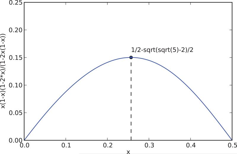
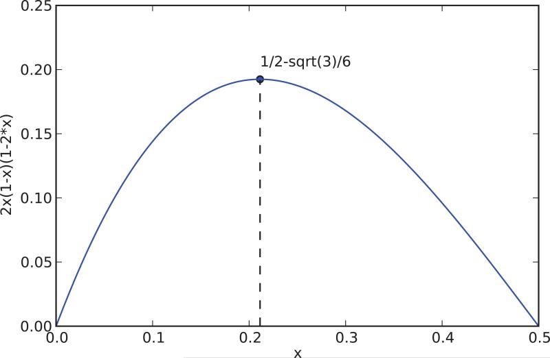
The inequalities are optimal in the sense that they are attained in the case of a Bernoulli variable with expectation E. The function E(1 – E)|1 – 2E|/[1 – 2E(1 – E)] is zero for E = 0, 0.5, or 1, and symmetric with respect to E = 0.5. It is convex down and its maximum over the interval [0, 0.5] is achieved for $E=0.5-\sqrt{\sqrt{5}-2}∕2$ (Figure 8.1). The function 2E(1 – E)|1 – 2E| is zero for E = 0, 0.5, or 1 , and symmetric with respect to E = 0.5. It is convex down and its maximum over the interval [0, 0.5] is achieved for $E=0.5-\sqrt{3}∕6$ (Figure 8.2). Note that at the beginning of learning, with small random weights initialization, typically E is close to 0.5. Towards the end of learning, E is often close to 0 or 1. In all these cases, the bounds are close to 0 and the NWGM is close to E.

Figure 8.1.

The curve associated with the approximate bound |E – NWGM| ≲ E(1 – E)|1 – 2E|/[1 – 2E(1 – E)] (Equation 87).

Figure 8.2.

The curve associated with the approximate bound |E – NWGM| ≲ 2E(1 – E)|1 – 2E| (Equation 87).

Note also that it is possible to have E = NWGM even when the numbers O_i are not identical. For instance, if O₁ = 0.25, O₂ = 0.75, and P₁ = P₂ = 0.5 we have G = G′ and thus: E = NWGM = 0.5.

In short, in general the NWGM is a better approximation to the expectation E than the geometric mean G. The property is always true to a second order of approximation. Furthermore, it is always exact when NWGM ≤ E since we must have G ≤ NWGM E. Furthermore, in general the NWGM is a better approximation to the mean than a random sample. Using a randomly chosen O_i as an estimate of the mean E, leads to an error that scales like the standard deviation $\sigma =\sqrt{V}$, whereas the NWGM leads to an error that scales like V.

When NWGM > E, “third order” cases can be found where

$$\frac{G}{G+G^{\prime }}-E\approx E-G\text{with}\frac{G}{G+G^{\prime }}-E\ge E-G$$ (88)

An example is provided by: O₁ = 0.622459, O₂ = 0.731059 with a uniform distribution (p₁ = p₂ = 0.5). In this case, E = 0.676759, G = 0.674577, G′ = 0.318648, NWGM = 0.679179, E – G = 0.002182 and NWGM – E = 0.002420.

Extreme Cases: Note also that if for some i, O_i = 1 with non-zero probability, then G′ = 0. In this case, NWGM = 1, unless there is a j ≠ i such that O_j = 0 with non-zero probability.

Likewise if for some i, O_i = 0 with non-zero probability, then G = 0. In this case, NWGM = 0, unless there is a j ≠ i such that O_j = 1 with non-zero probability. If both O_i = 1 and O_j = 0 are achieved with non-zero probability, then NWGM = 0/0 is undefined. In principle, in a sigmoidal neuron, the extreme output values 0 and 1 are never achieved, although in simulations this could happen due to machine precision. In all these extreme cases, where the NWGM is a good approximation of E or not depends on the exact distribution of the values. For instance, if for some i, O_i = 1 with non-zero probability, and all the other O_j's are also close to 1, then NWGM = 1 ≈ E. On the other hand, if O_i = 1 with small but non-zero probability, and all the other O_j's are close to 0, then NWGM = 1 is not a good approximation of E.

Higher Order Moments: It would be useful to be able to derive estimates also for the variance V, as well as other higher order moments of the numbers O, especially when O = σ(S). While the NWGM can easily be generalized to higher order moments, it does not seem to yield simple estimates as for the mean (see Appendix). However higher order moments in a deep network trained with dropout can easily be approximated, as in the linear case (see Section 9).

Proof: To prove these results, we compute first and second order approximations. Depending on the case of interest, the numbers 0 < O_i < 1 can be expanded around E, around G, or around 0.5 (or around 0 or 1 when they are consistently close to these boundaries). Without assuming that they are consistently low or high, we expand them around 0.5 by writing O_i = 0.5 + ε_i where 0 ≤ |ε_i| ≤ 0.5. [Estimates obtained by expanding around E are given in the Appendix]. For any distribution P₁, . . . , P_m over the m subnetworks, we have E(O) = 0.5 + E(ε) and Var(O) = Var(ε). As usual, let $G={\prod }_i{O}_i^{P_i}={\prod }_i(0.5+{∊}_i)P_i=0.5{\prod }_i(1+2{∊}_i)P_i$. To a first order of approximation,

$$G=\prod _{i=1}^m{(\frac{1}{2}+{∊}_i)}^{P_i}=\frac{1}{2}\prod _{i=1}^m{(1+2{∊}_i)}^{P_i}\approx \frac{1}{2}+\sum _{i=1}^m{P}_i{∊}_i=E$$ (89)

The approximation is obtained using a Taylor expansion and the fact that 2|ε_i| < 1. In a similar way, we have G′ ≈ 1 – E and G/(G + G′) ≈ E. These approximations become more accurate as ε_i → 0. To a second order of approximation, we have

$$G=\frac{1}{2}\prod _i\sum _{n=0}^{\infty }\left(\begin{array}{c}\hfill P_i\hfill \\ \hfill n\hfill \end{array}\right){\left(2{∊}_i\right)}^n=\frac{1}{2}\prod _i\left[1+P_{i}2{∊}_i+\frac{P_i(P_i-1)}{2}{\left(2{∊}_i\right)}^2+R_3\left({∊}_i\right)\right]$$ (90)

where R₃(ε_i) is the remainder of order three

$$R_3\left({∊}_i\right)=\left(\begin{array}{c}\hfill P_i\hfill \\ \hfill 3\hfill \end{array}\right)\frac{{\left(2{∊}_i\right)}^3}{{(1+u_i)}^{3-P_i}}=o\left({∊}_i^2\right)$$ (91)

and |u_i| ≤ 2|ε_i|. Expanding the product gives

$$G=\frac{1}{2}\prod _i\sum _{n=0}^{\infty }\left(\begin{array}{c}\hfill P_i\hfill \\ \hfill n\hfill \end{array}\right){\left(2{∊}_i\right)}^n=\frac{1}{2}\left[1+\sum _i{P}_{i}2{∊}_i+\sum _i\frac{P_i(P_i-1)}{2}{\left(2{∊}_i\right)}^2+\sum _{i<j}4P_i{P}_j{∊}_i{∊}_j+R_3\left(∊\right)\right]$$ (92)

which reduces to

$$G=\frac{1}{2}+\sum _i{P}_i{∊}_i+{\left(\sum _i{P}_i{∊}_i\right)}^2-\sum P_i{∊}_i^2+o\left({∊}^2\right)=\frac{1}{2}+E\left(∊\right)-Var\left(∊\right)+o\left({∊}^2\right)=E\left(O\right)-Var\left(O\right)+R_3\left(∊\right)$$ (93)

By symmetry, we also have

$$G^{\prime }=\prod _i{(1-O_i)}^{P_i}=1-E\left(O\right)-Var\left(O\right)+R_3\left(∊\right)$$ (94)

where again R₃(ε) is the higher order remainder. Neglecting the remainder and writing E = E(O) and V = Var(O) we have

$$\frac{G}{G+G^{\prime }}\approx \frac{E-V}{1-2V}\text{and}\frac{G^{\prime }}{G+G^{\prime }}\approx \frac{1-E-V}{1-2V}$$ (95)

Thus the differences between the mean on one hand, and the geometric mean and the normalized geometric means on the other, satisfy

$$E-G\approx V\text{and}E-\frac{G}{G+G^{\prime }}\approx \frac{V(1-2E)}{1-2V}$$ (96)

and

$$1-E-G^{\prime }\approx V\text{and}(1-E)-\frac{G^{\prime }}{G+G^{\prime }}\approx \frac{V(1-2E)}{1-2V}$$ (97)

To know when the NWGM is a better approximation to E than the WGM, we consider when the factor |(1 – 2E)/(1 – 2V)| is less or equal to one. There are four cases:

1. E ≤ 0.5 and V ≤ 0.5 and E ≥ V.

2. E ≤ 0.5 and V ≥ 0.5 and E + V ≥ 1.

3. E ≥ 0.5 and V ≤ 0.5 and E + V ≤ 1.

4. E ≥ 0.5 and V ≥ 0.5 and E ≤ V.

However, since 0 < O_i < 1, we have V ≤ E – E² = E(1 – E) ≤ 0.25. So only cases 1 and 3 are possible and in both cases the relationship is trivially satisfied. Thus in all cases, to a second order of approximation, the NWGM is closer to E than the WGM.

9 Dropout Distributions and Approximation Properties

Throughout the rest of this article, we let $W_i^l=\sigma \left(U_i^l\right)$ denote the deterministic variables of the dropout approximation (or ensemble network) with

$$W_i^l=\sigma \left(\sum _{h<l}\sum _j{w}_{ij}^{hl}{p}_j^h{W}_j^h\right)$$ (98)

in the case of dropout applied to the nodes. The main question we wish to consider is whether $W_i^l$ is a good approximation to $E\left(O_i^l\right)$ for every input, every layer l, and any unit i.

9.1 Dropout Induction

Dropout relies on the correctness of the approximation of the expectation of the activity of each unit over all its dropout subnetworks by the corresponding deterministic variable in the form

$$W_i^l\approx E\left(O_i^l\right)$$ (99)

for each input, each layer l, and each unit i. The correctness of this approximation can be seen by induction. For the first layer, the property is obvious since $W_i^l=NWGM\left(O_i^l\right)\approx E\left(O_i^l\right)$, using the results of Section 8. Now assume that the property is true up to layer l. Again, by the results in Section 8,

$$E\left(O_i^{l+1}\right)\approx NWGM\left(O_i^{l+1}\right)=\sigma \left(E\left(S_i^{l+1}\right)\right)$$ (100)

which can be computed by

$$\sigma \left(E\left(S_i^{l+1}\right)\right)=\sigma \left(\sum _{h<l+1}\sum _j{w}_{ij}^{l+1h}{p}_j^{h}E\left(O_j^h\right)\right)\approx \sigma \left(\sum _{h<l+1}\sum _j{w}_{ij}^{l+1h}{p}_j^h{W}_j^h\right)=W_i^{l+1}$$ (101)

The approximation in Equation 101 uses of course the induction hypothesis. This induction, however, does not provide any sense of the errors being made, and whether these errors increase significantly with the depth of the networks. The error can be decomposed into two terms

$${∊}_i^l=E\left(O_i^l\right)-W_i^l=[E\left(O_i^l\right)-NWGM\left(O_i^l\right)]+[NWGM\left(O_i^l\right)-W_i^l]={\alpha }_i^l+{\beta }_i^l$$ (102)

Thus in what follows we study each term.

9.2 Sampling Distributions

In Section 8, we have shown that in general NWGM(O) provides a good approximation to E(O). To further understand the dropout approximation and its behavior in deep networks, we must look at the distribution of the difference α = E(O) – NWGM(O). Since both E and NWGM are deterministic functions of a set of O values, a distribution can only be defined if we look at different samples of O values taken from a more general distribution. These samples could correspond to dropout samples of the output of a given neuron. Note that the number of dropout subnetworks of a neuron being exponentially large, only a sample can be accessed during simulations of large networks. However, we can also consider that these samples are associated with a population of neurons, for instance the neurons in a given layer. While we cannot expect the neurons in a layer to behave homogeneously for a given input, they can in general be separated in a small number of populations, such as neurons that have low activity, medium activity, and high activity and the analysis below can be applied to each one of these populations separately. Letting $O_{\mathcal{S}}$ denote a sample of m values O_i, . . . , O_m, we are going to show through simulations and more formal arguments that in general $E\left(O_{\mathcal{S}}\right)-NWGM\left(O_{\mathcal{S}}\right)$ has a mean close to 0, a small standard deviation, and in many cases is approximately normally distributed. For instance, if the O originate from a uniform distribution over [0.1], it is easy to see that both E and NWGM are approximately normally distributed, with mean 0.5, and a small variance decreasing as 1/m.

9.3 Mean and Standard Deviation of the Normalized Weighted Geometric Mean

More generally, assume that the variables O_i are i.i.d with mean μ_O and variance ${\sigma }_O^2$. Then the variables S_i satisfying O_i = σ(S_i) are also i.i.d. with mean μ_S and variance ${\sigma }_S^2$. Densities for S when O has a Beta distribution, or for O when S has a Gaussian distribution, are derived in the Appendix. These could be used to model in more detail non uniform distributions, and distributions corresponding to low or high activity. For m sufficiently large, by the central limit theorem² the means of these quantities are approximately normal with:

$$E\left(O_{\mathcal{S}}\right)\sim \mathcal{N}({\mu }_O,\frac{{\sigma }_O^2}{m})\text{and}E\left(S_{\mathcal{S}}\right)\sim \mathcal{N}({\mu }_{\mathcal{S}},\frac{{\sigma }_S^2}{m})$$ (103)

If these standard deviations are small enough, which is the case for instance when m is large, then σ can be well approximated by a linear function with slope t over the corresponding small range. In this case, $NWGM\left(O_{\mathcal{S}}\right)=\sigma \left(E\left(S_{\mathcal{S}}\right)\right)$ is also approximately normal with

$$NWGM\left(O_{\mathcal{S}}\right)\sim \mathcal{N}(\sigma \left({\mu }_S\right),\frac{t^2{\sigma }_S^2}{m})$$ (104)

Note that |t| ≤ λ/4 since σ′ = λσ(1 – σ). Very often, σ(μ_S) ≈ μ_O. This is particularly true if μ_O = 0.5. Away from 0.5, a bias can appear—for instance we know that if all the O_i < 0.5 then NWGM < E—but this bias is relatively small. This is confirmed by simulations, as shown in Figure 9.1 using Gaussian or uniform distributions to generate the values O_i. Finally, note that the variance of $E\left(O_{\mathcal{S}}\right)$ and $NWGM\left(O_{\mathcal{S}}\right)$ are of the same order and behave like C₁/m and C₂/m respectively as m → ∞. Furthermore ${\sigma }_O^2=C_1\approx C_2$ if ${\sigma }_O^2$ is small.

Figure 9.1.

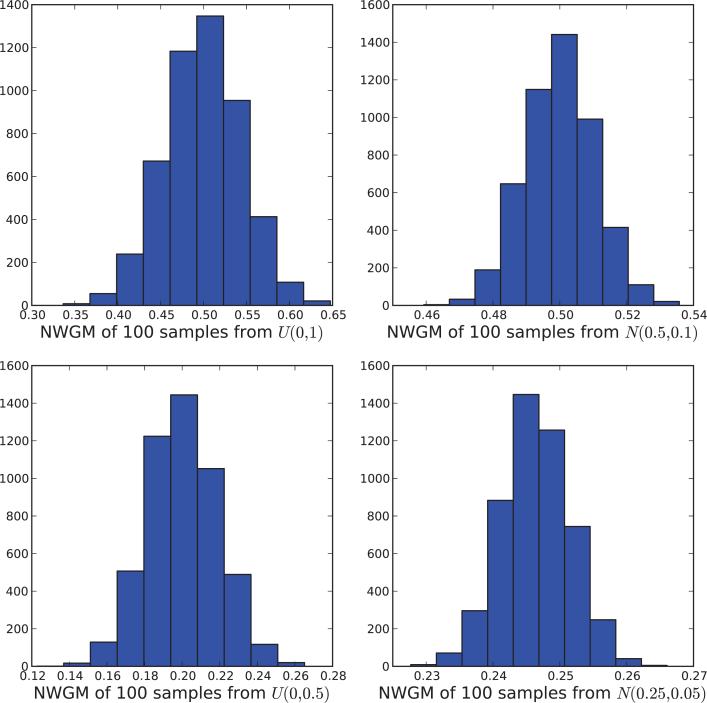
Histogram of NWGM values for a random sample of 100 values O taken from: (1) the uniform distribution over [0,1] (upper left); (2) the uniform distribution over [0,0.5] (lower left); (3) the normal distribution with mean 0.5 and standard deviation 0.1 (upper right); and (4) the normal distribution with mean 0.25 and standard deviation 0.05 (lower right). All probability weights are equal to 1/100. Each sampling experiment is repeated 5,000 times to build the histogram.

If necessary, it is also possible to derive better and more general estimates of E(O), under the assumption that S is Gaussian by approximating the logistic function with the cumulative distribution of a Gaussian, as described in the Appendix (see also [41]).

If we sample from many neurons whose activities come from the same distribution, the sample mean and the sample NWGM will be normally distributed and have roughly the same mean. The difference will have approximately zero mean. To show that the difference is approximately normal we need to show that E and NWGM are uncorrelated.

9.4 Correlation between the Mean and the Normalized Weighted Geometric Mean

We have

$$Var\left[E\left(O_{\mathcal{S}}\right)\right]-NWGM\left[O{}_{\mathcal{S}})\right]=Var\left[E\left(O_{\mathcal{S}}\right)\right]+Var\left[NWGM\left(O_{\mathcal{S}}\right)\right]+2Cov[E\left(O_{\mathcal{S}}\right),NWGM\left(O_{\mathcal{S}}\right)]$$ (105)

Thus to estimate the variance of the difference, we must estimate the covariance between $E\left(O_{\mathcal{S}}\right)$ and $NWGM\left(O_{\mathcal{S}}\right)$. As we shall see, this covariance is close to null.

In this section, we assume again samples of size m from a distribution on O with mean E = μ_O and variance $V={\sigma }_O^2$. To simplify the notation, we use $E_{\mathcal{S}}$, $V_{\mathcal{S}}$, and $NWG{M}_{\mathcal{S}}$ to denote the random variables corresponding to the mean, variance, and normalized weighted geometric mean of the sample. We have seen, by doing a Taylor expansion around 0.5, that $NWG{M}_{\mathcal{S}}\approx (E_{\mathcal{S}}-V_{\mathcal{S}})∕(1-2V_{\mathcal{S}})$.

We first consider the case where E = NWGM = 0.5. In this case, the covariance of $NWG{M}_{\mathcal{S}}$ and $E_{\mathcal{S}}$ can be estimated as

$$Cov(NWG{M}_{\mathcal{S}},E_{\mathcal{S}})\approx E\left[\left(\frac{E_{\mathcal{S}}-V_{\mathcal{S}}}{1-2V_{\mathcal{S}}}-\frac{1}{2}\right)\left(E_{\mathcal{S}}-\frac{1}{2}\right)\right]=E\left[\frac{{(E-\frac{1}{2})}^2}{1-2V_{\mathcal{S}}}\right]$$ (106)

We have $0.5\le 1-2V_{\mathcal{S}}\le 1$ and $E{(E_{\mathcal{S}}-\frac{1}{2})}^2=Var\left(E_{\mathcal{S}}\right)=V∕m$. Thus in short the covariance is of order V/m and goes to 0 as the sample size m goes to infinity. For the Pearson correlation, the denominator is the product of two similar standard deviations and scales also like V/m. Thus the correlation should be roughly constant and close to 1. More generally, even when the mean E is not equal to 0.5, we still have the approximations

$$Cov(NWG{M}_{\mathcal{S}},E_{\mathcal{S}})\approx E\left[\left(\frac{E_{\mathcal{S}}-V_{\mathcal{S}}}{1-2V_{\mathcal{S}}}-\frac{E-V}{1-2V}\right)(E_{\mathcal{S}}-E)\right]=E\left[\frac{{(E-E_{\mathcal{S}})}^2+(V-V_{\mathcal{S}})(E_{\mathcal{S}}-E)}{(1-2V_{\mathcal{S}})(1-2V)}\right]$$ (107)

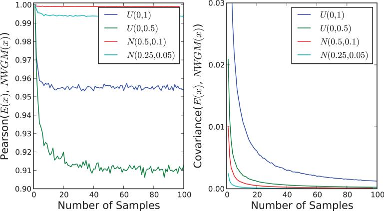
And the leading term is still of order V/m [Similar results are also obtained by using the expansions around 0 or 1 given in the Appendix to model populations of neurons with low or high activity]. Thus again the covariance between NWGM and E goes to 0, and the Pearson correlation is constant and close to 1. These results are confirmed by simulations in Figure 9.2.

Figure 9.2.

Behavior of the Pearson correlation coefficient (left) and the covariance (right) between the empirical expectation E and the empirical NWGM as a function of the number of samples and sample distribution. For each number of samples, the sampling procedure is repeated 10,000 times to estimate the Pearson correlation and covariance. The distributions are the uniform distribution over [0,1], the uniform distribution over [0,0.5], the normal distribution with mean 0.5 and standard deviation 0.1, and the normal distribution with mean 0.25 and standard deviation 0.05.

Combining the previous results we have

$$Var(E_{\mathcal{S}}-NWG{M}_{\mathcal{S}})\approx Var\left(E_{\mathcal{S}}\right)+Var\left(NWG{M}_{\mathcal{S}}\right)\approx \frac{C_1}{m}+\frac{C_2}{m}$$ (108)

Thus in general $E\left(O_{\mathcal{S}}\right)$and $NWGM\left(O_{\mathcal{S}}\right)$ are random variables with: (1) similar, if not identical, means; (2) variances and covariance that decrease to 0 inversely to the sample size; (3) approximately normal distributions. Thus E – NWGM is approximately normally distributed around zero. The NWGM behaves like a random variable with small fluctuations above and below the mean. [Of course contrived examples can be constructed (for instance with small m or small networks) which deviate from this general behavior.]

9.5 Dropout Approximations: the Cancellation Effects

To complete the analysis of the dropout approximation of $E\left(O_i^l\right)$ by $W_i^l$, we show by induction over the layers that $W_i^l=E\left(O_i^l\right)-{∊}_i^l$ where in general the error term ${∊}_i^l={\alpha }_i^l+{\beta }_i^l$ is small and approximately normally distributed with mean 0. Furthermore the error ${∊}_i^l$ is uncorrelated with the error ${\alpha }_i^l=E\left(O_i^l\right)-NWGM\left(O_i^l\right)$ for l > 1.

First, the property is true for l = 1 since $W_i^l=NWGM\left(O_i^l\right)$ and the results of the previous sections apply immediately to this case. For the induction step, we assume that the property is true up to layer l. At the following layer, we have

$$W_i^{l+1}=\sigma \left(\sum _{h\le l}\sum _j{w}_{ij}^{l+1h}{p}_j^h{W}_j^h\right)=\sigma \left(\sum _{h\le l}\sum _j{w}_{ij}^{l+1h}{p}_j^h[E\left(O_j^h\right)-{∊}_j^h]\right)$$ (109)

Using a first order Taylor expansion

$$W_i^{l+1}\approx NWGM\left(O_i^{l+1}\right)+{\sigma }^{\prime }\left(\sum _{h\le l}\sum _j{w}_{ij}^{l+1h}{p}_j^{h}E\left(O_j^h\right)\right)[-\sum _{h\le l}\sum _j{w}_{ij}^{l+1h}{p}_j^h{∊}_j^h]$$ (110)

or more compactly

$$W_i^{l+1}\approx NWGM\left(O_i^{l+1}\right)-{\sigma }^{\prime }\left(E\left(S_i^{l+!}\right)\right)\left[\sum _{h\le l}\sum _j{w}_{ij}^{l+1h}{p}_j^h{∊}_j^h\right]$$ (111)

thus

$${\beta }_i^{l+1}=NWGM\left(O_i^{l+1}\right)-W_i^{l+1}\approx {\sigma }^{\prime }\left(E\left(S_i^{l+1}\right)\right)\left[\sum _{h\le l}\sum _j{w}_{ij}^{l+1h}{p}_j^h{∊}_j^h\right]$$ (112)

As a sum of many linear small terms, ${\beta }_i^{l+1}$ is approximately normally distributed. By linearity of the expectation

$$E\left({\beta }_i^{l+1}\right)\approx 0$$ (113)

By linearity of the variance with respect to sums of independent random variables

$$Var{({\beta }_i^{l+1}\approx [{\sigma }^{\prime }\left(E\left(S_i^{l+1}\right)\right)]}^2\sum _{h\le l}\sum _j{\left(w_{ij}^{l+1h}\right)}^2{\left(p_j^h\right)}^{2}Var\left({∊}_j^h\right)]$$ (114)

This variance is small since ${\left[{\sigma }^{\prime }\left(E\left(S_i^{l+1}\right)\right)\right]}^2\le 1∕16$ for the standard logistic function (and much smaller than 1/16 at the end of learning, ${\left(p_j^h\right)}^2\le 1$, and $Var\left({∊}_j^h\right)$ is small by induction. The weights $w_{ij}^{l+1h}$ are small at the beginning of learning and as we shall see in Section 11 dropout performs weight regularization automatically. While this is not observed in the simulations used here, one concern is that with very large layers the sum could become large. We leave a more detailed study of this issue for future work. Finally, we need to show that ${\alpha }_i^{l+1}$ and ${\beta }_i^{l+1}$ are uncorrelated. Since both terms have approximately mean 0, we compute the mean of their product

$$E\left({\alpha }_i^{l+1}{\beta }_i^{l+1}\right)\approx E\left[(E\left(O_i^{l+1}\right)-NWGM\left(O_i^{l+1}\right)){\sigma }^{\prime }\left(E\left(S_i^{+1}\right)\right)\sum _{h\le l}\sum _j{w}_{ij}^{l+1h}{p}_j^h{∊}_j^h\right]$$ (115)

By linearity of the expectation

$$E\left({\alpha }_i^{l+1}{\beta }_i^{l+1}\right)\approx {\sigma }^{\prime }\left(E\left(S_i^{l+1}\right)\right)\sum _{h\le l}\sum _j{w}_{ij}^{l+1h}{p}_j^{h}E\left[(E\left(O_i^{l+1}\right)-NWGM\left(O_i^{l+1}\right)){∊}_j^h\right]\approx 0$$ (116)

since $E[E\left(O_i^{l+1}\right)-NWGM\left(O_i^{l+1}\right)){∊}_j^h=E[E\left(O_i^{l+1}\right)-NWGM\left(O_i^{l+1}\right)]E\left({∊}_j^h\right)\approx 0$

In summary, in general both $W_i^l$ and $NGWM\left(O_i^l\right)$ can be viewed as good approximations to $E\left(O_i^l\right)$ with small deviations that are approximately Gaussians with mean zero and small standard deviations. These deviations act like noise and cancel each other to some extent preventing the accumulation of errors across layers.

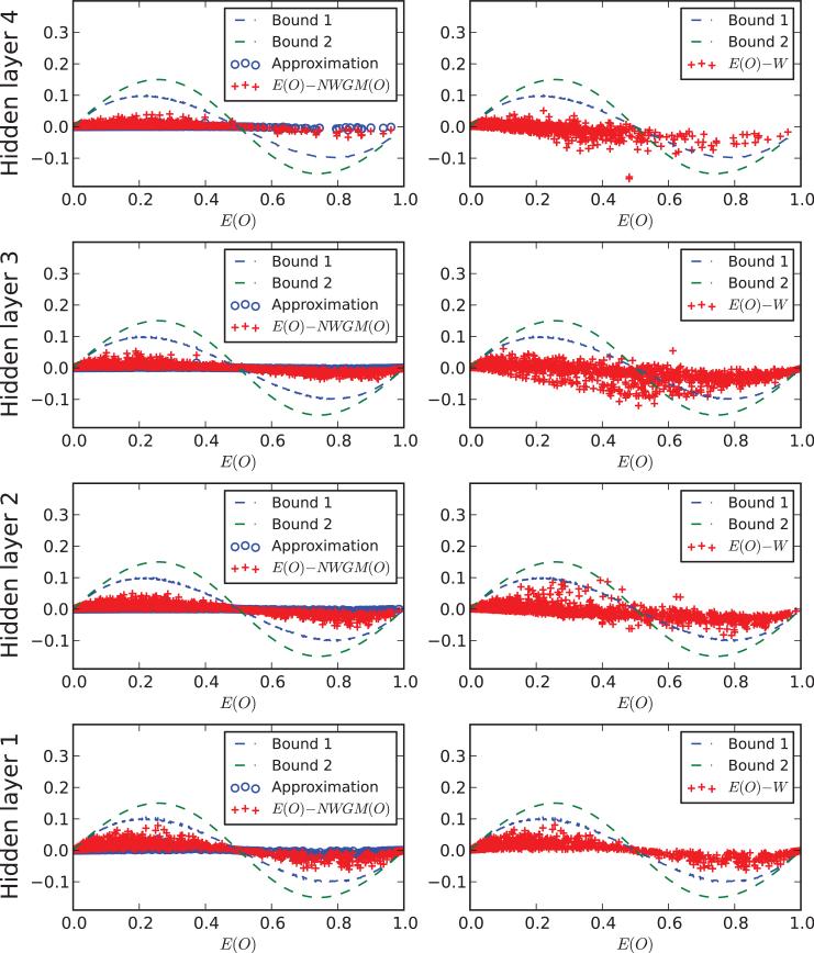
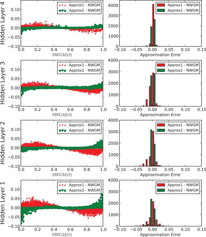
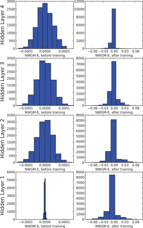
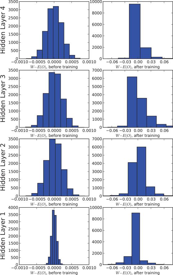
These results and those of the previous section are confirmed by simulation results given by Figures 9.3, 9.4, 9.5, 9.6, and 9.7. The simulations are based on training a deep neural network classifier on the MNIST handwritten characters dataset with layers of size 784-1200-1200-1200-1200-10 replicating the results described in [27], using p = 0.8 for the input layer and p = 0.5 for the hidden layers. The raster plots accumulate the results obtained for 10 randomly selected input vectors. For fixed weights and a fixed input vector, 10,000 Monte Carlo simulations are used to sample the dropout subnetworks and estimate the distribution of activities O of each neuron in each layer. These simulations use the weights obtained at the end of learning, except in the cases were the beginning and end of learning are compared (Figures 9.6 and 9.7). In general, the results show how well the $NWGM\left(O_i^l\right)$ and the deterministic values $W_i^l$ approximate the true expectation $E\left(O_i^l\right)$ in each layer, both at the beginning and the end of learning, and how the deviations can roughly be viewed as small, approximately Gaussian, fluctuations well within the bounds derived in Section 8.

Figure 9.3.

Each row corresponds to a scatter plot for all the neurons in each one of the four hidden layers of a deep classifier trained on the MNIST dataset (see text) after learning. Scatter plots are derived by cumulating the results for 10 random chosen inputs. Dropout expectations are estimated using 10,000 dropout samples. The second order approximation in the left column (blue dots) correspond to |E – NWGM| ≈ V|1 – 2E|/(1 – 2V) (Equation 87). Bound 1 is the variance-dependent bound given by E(1 – E)|1 – 2E|/(1 – 2V) (Equation 87). Bound 2 is the variance-independent bound given by E(1–E)|1–2E|/(1–2E(1–E)) (Equation 87). In the right column, W represent the neuron activations in the deterministic ensemble network with the weights scaled appropriately and corresponding to the “propagated” NWGMs.

Figure 9.4.

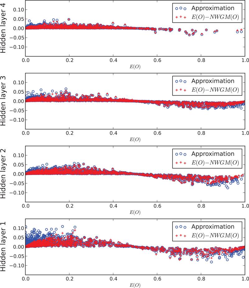
Similar to Figure 9.3, using the sharper but potentially more restricted second order approximation to the NWGM obtained by using a Taylor expansion around the mean (see Appendix B, Equation 202).

Figure 9.5.

Similar to Figures 9.3 and 9.4. Approximation 1 corresponds to the second order Taylor approximation around 0.5: ∥E – NWGM| ≈ V|1 – 2E|/(1 – 2V) (Equation 87). Approximation 2 is the sharper but more restrictive second order Taylor approximation around $E:\frac{E-(V∕2E)}{1-(\left[0.5V\right]∕\left[E(1-E)\right])}$ (see Appendix B, Equation 202). Histograms for the two approximations are interleaved in each figure of the right column.

Figure 9.6.

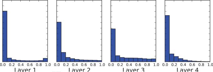
Empirical distribution of NWGM – E is approximately Gaussian at each layer, both before and after training. This was performed with Monte Carlo simulations over dropout subnetworks with 10,000 samples for each of 10 fixed inputs. After training, the distribution is slightly asymmetric because the activation of the neurons is asymmetric. The distribution in layer one before training is particularly tight simply because the input to the network (MNIST data) is relatively sparse.

Figure 9.7.

Empirical distribution of W – E is approximately Gaussian at each layer, both before and after training. This was performed with Monte Carlo simulations over dropout subnetworks with 10,000 samples for each of 10 fixed inputs. After training, the distribution is slightly asymmetric because the activation of the neurons is asymmetric. The distribution in layer one before training is particularly tight simply because the input to the network (MNIST data) is relatively sparse.

9.6 Dropout Approximations: Estimation of Variances and Covariances

We have seen that the deterministic values W s can be used to provide very simple but effective estimates of the values E(O)s across an entire network under dropout. Perhaps surprisingly, the W s can also be used to derive approximations of the variances and covariances of the units as follows.

First, for the dropout variance of a neuron, we can use

$$E\left(O_i^l{O}_i^l\right)\approx W_i^l\text{or equivalently}Var\left(O_i^l\right)\approx W_i^l(1-W_i^l)$$ (117)

or

$$E\left(O_i^l{O}_i^l\right)\approx W_i^l{W}_i^l\text{or equivalently}Var\left(O_i^l\right)\approx 0$$ (118)

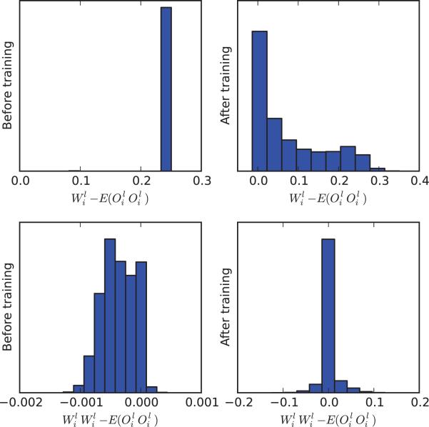
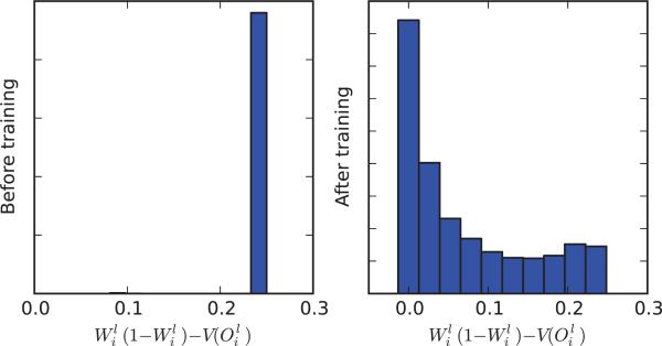
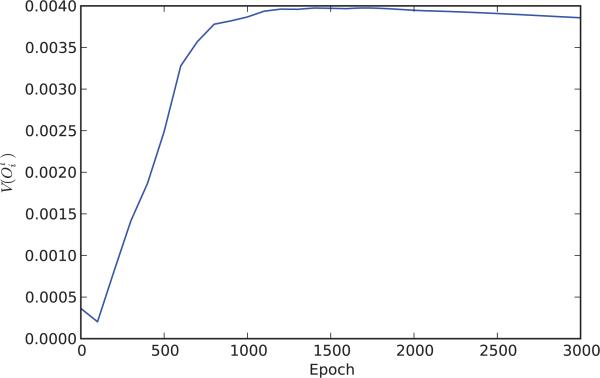
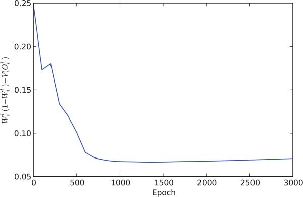
These two approximations can be viewed respectively as rough upperbounds and lower bounds to the variance. For neurons whose activities are close to 0 or 1, and thus in general for neurons towards the end of learning, these two bounds are similar to each other. This is not the case at the beginning of learning when, with very small weights and a standard logistic transfer function, $W_i^l=0.5$ and $Var\left(O_i^l\right)\approx 0$ (Figure 9.8 and 9.9). At the beginning and the end of learning, the variances are small and so “0” is the better approximation. However , during learning, variances can be expected to be larger and closer to their approximate upper bound W(1 – W) (Figures 9.10 and 9.11).

Figure 9.8.

Approximation of $E\left(O_i^l{O}_i^l\right)$ by $W_i^l$ and by $W_i^l{W}_i^l$ corresponding respectively to the estimates $W_i^l(1-W_i^l)$ and for the variance for neurons in a MNIST classifier network before and after training. Histograms are obtained by taking all non-input neurons and aggregating the results over 10 random input vectors.

Figure 9.9.

Histogram of the difference between the dropout variance of $O_i^l$ and its approximate upperbound $W_i^l\left(W_i^l\right)$ in a MNIST classifier network before and after training. Histograms are obtained by taking all non-input neurons and aggregating the results over 10 random input vectors. Note that at the beginnning of learning, with random small weights, $E\left(O_i^l\right)\approx W_i^l\approx 0.5$, and thus $Var\left(O_i^l\right)\approx 0$ whereas $W_i^l(1-W_i^l)\approx 0.25$.

Figure 9.10.

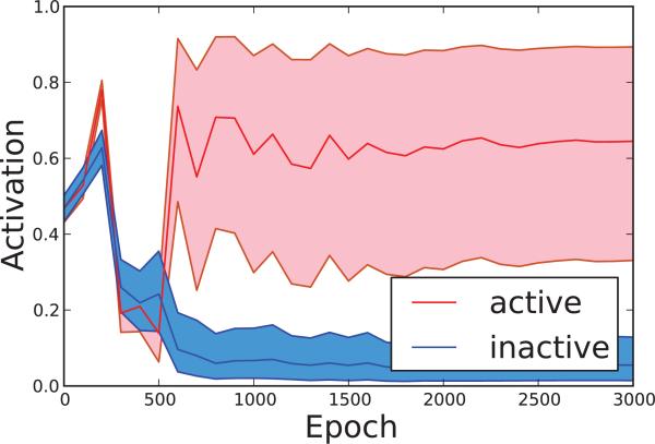
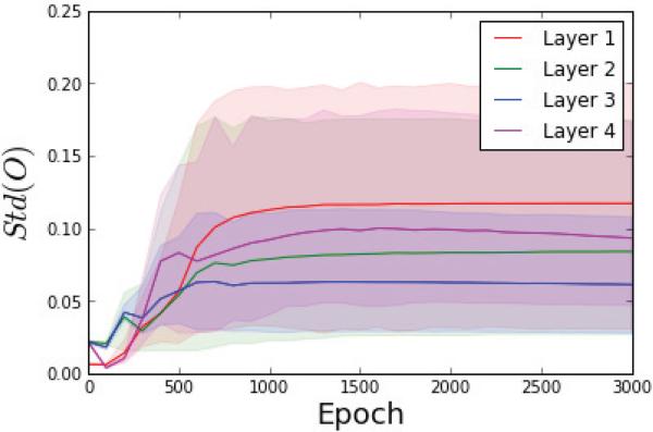
Temporal evolution of the dropout variance V(O) during training averaged over all hidden units.

Figure 9.11.

Temporal evolution of the difference W(1 – W ) – V during training averaged over all hidden units.

For the covariances of two different neurons, we use

$$E\left(O_i^l{O}_j^h\right)=E\left(O_i^l\right)E\left(O_j^h\right)\approx W_i^l{W}_j^h$$ (119)

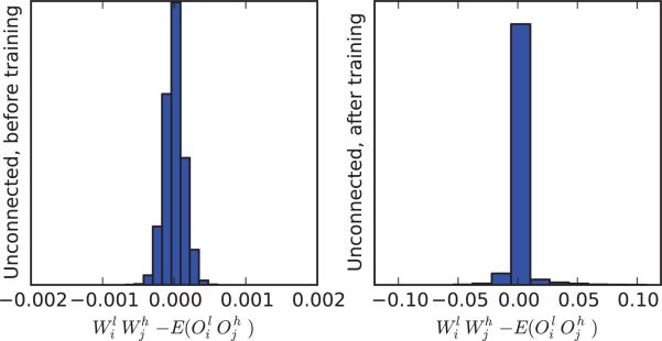
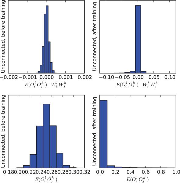
This independence approximation is accurate for neurons that are truly independent of each other, such as pairs of neurons in the first layer. However it can be expected to remain approximately true for pairs of neurons that are only loosely coupled, i.e. for most pairs of neurons in a large neural networks at all times during learning. This is confirmed by simulations (Figure 9.12) conducted using the same network trained on the MNIST dataset. The approximation is much better than simply using 0 (Figure 9.13).

Figure 9.12.

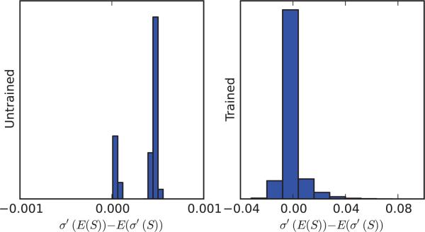
Approximation of $E\left(O_i^l{O}_j^h\right)$ by $W_i^l{W}_j^h$ for pairs of non-input neurons that are not directly connected to each other in a MNIST classifier network, before and after training. Histograms are obtained by taking 100,000 pairs of unconnected neurons, uniformly at random, and aggregating the results over 10 random input vectors.

Figure 9.13.

Comparison of $E\left(O_i^l{O}_j^h\right)$ to 0 for pairs of non-input neurons that are not directly connected to each other in a MNIST classifier network, before and after training. As shown in the previous figure, $W_i^l{W}_j^h$ provides a better approximation. Histograms are obtained by taking 100,000 pairs of unconnected neurons, uniformly at random, and aggregating the results over 10 random input vectors.

For neurons that are directly connected to each other, this approximation still holds but one can try to improve it by introducing a slight correction. Consider the case of a neuron with output $O_j^h$ feeding directly into the neuron with output $O_i^l(h<l)$ through a weight $w_{ij}^{lh}$. By isolating the contribution of $O_j^h$, we have

$$O_i^l=\sigma (\sum _{f<l}\sum _{k\ne j}{w}_{ik}^{lf}{\sigma }_k^f{O}_k^f+w_{ij}^{lh}{\sigma }_j^h{O}_j^h)\approx \sigma \left(\sum _{f<l}\sum _{k\ne j}{w}_{ik}^{lf}{\sigma }_k^f{O}_k^f\right)+{\sigma }^{\prime }\left(\sum _{f<l}\sum _{k\ne j}{w}_{ik}^{lf}{\sigma }_k^f{O}_k^f\right)w_{ij}^{lh}{\delta }_j^h{O}_j^h$$ (120)

with a first order Taylor approximation which is more accurate when $w_{ij}^{lh}$ or $O_j^h$ are small (conditions that are particularly well satisfied at the beginning of learning or with sparse coding). In this expansion, the first term is independent of $O_j^h$ and its expectation can easily be computed as

$$E\left(\sigma \left(\sum _{f<l}\sum _{k\ne j}{w}_{ik}^{lf}{\delta }_k^f{O}_k^f\right)\right)\approx \sigma \left(E\left(\sum _{f<l}\sum _{k\ne j}{w}_{ik}^{lf}{\delta }_k^f{O}_k^f\right)\right)=\sigma \left(\sum _{f<l}\sum _{k\ne j}{w}_{ik}^{lf}{p}_k^f{W}_k^f\right)=W_{ij}^{lh}$$ (121)

Thus here $W_{ij}^{lh}$ is simply the deterministic activation of neuron i in layer l in the ensemble network when neuron j in layer h is removed from its inputs. Thus it can easily be computed by forward propagation in the deterministic network. Using a first-order Taylor expansion it can be estimated by

$$W_{ij}^{lh}\approx W_i^l-{\sigma }^{\prime }\left(U_i^l\right)w_{ij}^{lh}{p}_j^h{W}_j^h$$ (122)

In any case,

$$E\left(O_i^l{O}_j^h\right)\approx W_{ij}^{lh}{W}_j^h+E\left({\sigma }^{\prime }\left(\sum _{f<l}\sum _{k\ne j}{w}_{ik}^{lf}{\delta }_k^f{O}_k^f\right)\right)w_{ij}^{lh}{p}_j^{h}E\left(O_j^h{O}_j^h\right)$$ (123)

Towards the end of learning, σ′ ≈ 0 and so the second term can be neglected. A slightly more precise estimate can be obtained by writing σ′ ≈ λσ when σ is close to 0, and σ′ ≈ λ(1 – σ) when σ is close to 1, replacing the corresponding expectation by $W_{ij}^{lh}$ or $1-W_{ij}^{lh}$. In any case, to a leading term approximation, we have

$$E\left(O_i^l{O}_j^h\right)\approx W_{ij}^{lh}{W}_j^h$$ (124)

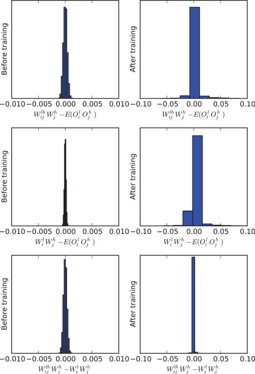
The accuracy of these formula for pairs of connected neurons is demonstrated in Figure 9.14 at the beginning and end of learning, where it is also compared to the approximation $E\left(O_i^l{O}_j^h\right)\approx W_i^l{W}_j^h$. The correction provides a small improvement at the end of learning but not at the beginning. This is because it neglects a term in σ′ which presumably is close to 0 at the end of learning. The improvement is small enough that for most purposes the simpler approximation $W_i^l{W}_j^h$ may be used in all cases, connected or unconnected.

Figure 9.14.

Approximation of $E\left(O_i^l{O}_j^h\right)$ by $W_i^l{W}_{ij}^{lh}$ and $W_i^l{W}_j^h$ for pairs of connected non-input neurons, with a directed connection from j to i in a MNIST classifier network, before and after training. Histograms are obtained by taking 100,000 pairs of connected neurons, uniformly at random, and aggregating the results over 10 random input vectors.

10 The Duality with Spiking Neurons and With Backpropagation

10.1 Spiking Neurons

There is a long-standing debate on the importance of spikes in biological neurons, and also in artificial neural networks, in particular as to whether the precise timing of spikes is used to carry information or not. In biological systems, there are many examples, for instance in the visual and motor systems, where information seems to be carried by the short term average firing rate of neurons rather than the exact timing of their spikes. However, other experiments have shown that in some cases the timing of the spikes are highly reproducible and there are also known examples where the timing of the spikes is crucial, for instance in the auditory location systems of bats and barn owls, where brain regions can detect very small interaural differences, considerably smaller than 1 ms [26, 19, 18]. However these seem to be relatively rare and specialized cases. On the engineering side the question of course is whether having spiking neurons is helpful for learning or any other purposes, and if so whether the precise timing of the spikes matters or not. There is a connection between dropout and spiking neurons which might shed some, at the moment faint, light on these questions.

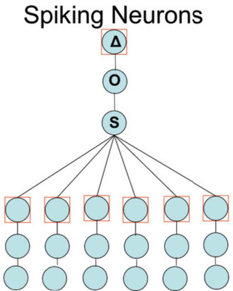
A sigmoidal neuron with output O = σ(S) can be converted into a stochastic spiking neuron by letting the neuron “flip a coin” and produce a spike with probability O. Thus in a network of spiking neurons, each neuron computes three random variables: an input sum S, a spiking probability O, and a stochastic output Δ (Figure 10.1). Two spiking mechanisms can be considered: (1) global: when a neuron spikes it sends the same quantity r along all its outgoing connections; and (2) local or connection-specific: when a neuron spikes with respect to a specific connection, it sends a quantity r along that connection. In the latter case, a different coin must be flipped for each connection. Intuitively, one can see that the first case corresponds to dropout on the units, and the second case to droupout on the connections. When a spike is not produced, the corresponding unit is dropped in the first case, and the corresponding connection is dropped in the second case.

Figure 10.1.

A spiking neuron formally operates in 3 steps by computing first a linear sum S, then a probability O = σ(S), then a stochastic output Δ of size r with probability O(and 0 otherwise).

To be more precise, a multi-layer network is described by the following equations. First for the spiking of each unit:

$${\Delta }_i^h=\{\begin{array}{cc}{r}_i^h\hfill & \text{with probability}{O}_i^h\hfill \\ 0\hfill & \text{otherwise}\hfill \end{array}\phantom{\}}$$ (125)

in the global firing case, and

$${\Delta }_{ji}^h=\{\begin{array}{cc}{r}_{ji}^h\hfill & \text{with probability}{O}_i^h\hfill \\ 0\hfill & \text{otherwise}\hfill \end{array}\phantom{\}}$$ (126)

in the connection-specific case. Here we allow the “size” of the spikes to vary with the neurons or the connections, with spikes of fixed-size being an easy special case. While the spike sizes could in principle be greater than one, the connection to dropout requires spike sizes of size at most one. The spiking probability is computed as usual in the form

$$O_i^h=\sigma \left(S_i^h\right)$$ (127)

and the sum term is given by

$$S_i^h=\sum _{l<h}\sum _j{w}_{ij}^{hl}{\Delta }_j^l$$ (128)

in the global firing case, and

$$S_i^h=\sum _{l<h}\sum _j{w}_{ij}^{hl}{\Delta }_{ij}^l$$ (129)

in the connection-specific case. The equations can be applied to all the layers, including the output layer and the input layer if these layers consist of spiking neurons. Obviously non-spiking neurons (e.g. in the input or output layers) can be combined with spiking neurons in the same network.

In this formalism, the issue of the exact timing of each spike is not really addressed. However some information about the coin flips must be given in order to define the behavior of the network. Two common models are to assume complete asynchrony, or to assume synchrony within each layer. As spikes propagate through the network, the average output E(Δ) of a spiking neuron over all spiking configurations is equal to r times the size its average firing probability E(O). As we have seen, the average firing probability can be approximated by the NWGM over all possible inputs S, leading to the following recursive equations:

$$E\left({\Delta }_i^h\right)=r_i^{h}E\left(O_i^h\right)$$ (130)

in the global firing case, or

$$E\left({\Delta }_{ji}^h\right)=r_{ji}^{h}E\left(O_i^h\right)$$ (131)

in the connection-specific case. Then

$$E\left(O_i^h\right)\approx NWGM\left(O_i^h\right)=\sigma \left(E\left(S_i^h\right)\right)$$ (132)

with

$$E\left(S_i^h\right)=\sum _{l<h}\sum _j{w}_{ij}^{hl}E\left({\Delta }_j^l\right)=\sum _{l<h}\sum _j{w}_{ij}^{hl}{r}_j^{l}E\left(O_j^l\right)$$ (133)

in the global firing case, or

$$E\left(S_i^h\right)=\sum _{l<h}\sum _j{w}_{ij}^{hl}E\left({\Delta }_{ij}^l\right)=\sum _{l<h}\sum _j{w}_{ij}^{hl}{r}_{ij}^{l}E\left(O_j^l\right)$$ (134)

in the connection-specific case.

In short, the expectation of the stochastic outputs of the stochastic neurons in a feedforward stochastic network can be approximated by a dropout-like deterministic feedforward propagation, proceeding from the input layer to the output layer, and multiplying each weight $w_{ij}^{hl}$ by the corresponding spike size $r_j^l\left(or{r}_{ij}^l\right)$–which acts as a dropout probability parameter– of the corresponding presynaptic neuron. [Operating a neuron in stochastic mode is also equivalent to setting all its inputs to 1 and using dropout on its connections with different Bernoulli probabilities associated with the sigmoidal outputs of the previous layer.]

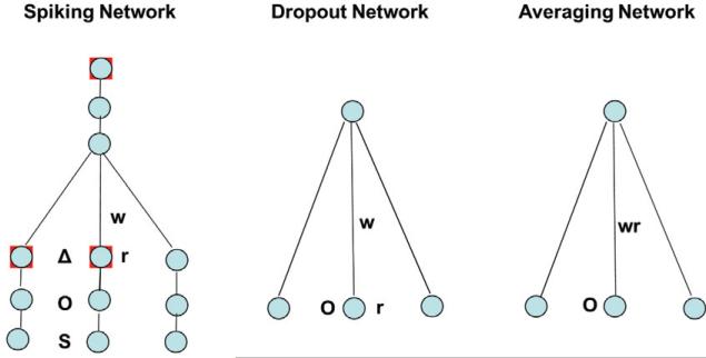
In particular, this shows that given any feedforward network of spiking neurons, with all spikes of size 1, we can approximate the average firing rate of any neuron simply by using deterministic forward propagation in the corresponding identical network of sigmoidal neurons. The quality of the approximation is determined by the quality of the approximations of the expectations by the NWGMs. More generally, consider three feedforward networks (Figure 10.2) with the same identical topology, and almost identical weights. The first network is stochastic, has weights $w_{ij}^{hl}$, and consists of spiking neurons: a neuron with activity $O_i^h$ sends a spike of size $r_i^h$ with probability $O_i^h$, and 0 otherwise (a similar argument can be made with connection-specific spikes of size $r_{ji}^h$). Thus, in this network neuron i in layer h sends out a signal that has instantaneous mean and variance given by

$$E=r_i^h{O}_i^h\text{and}Var={\left(r_i^h\right)}^2{O}_i^h(1-O_i^h)$$ (135)

for fixed $O_i^h$, and short-term mean and variance given by

$$E=r_i^{h}E\left(O_i^h\right)\text{and}Var={\left(r_i^h\right)}^{2}E\left(O_i^h\right)(1-E\left(O_i^h\right))$$ (136)

when averaged over all spiking configurations, for a fixed input.

Figure 10.2.

Three closely related networks. The first network operates stochastically and consists of spiking neurons: a neuron sends a spike of size r with probability O. The second network operates stochastically and consists of logistic dropout neurons: a neurons sends an activation O with a dropout probability r. The connection weights in the first and second networks are identical. The third network operates in a deterministic way and consists of logistic neurons. Its weights are equal to the weights of the second network multiplied by the corresponding probability r.

The second network is also stochastic, has identical weights to the first network, and consists of dropout sigmoidal neurons: a neuron with activity $O_i^h$ sends a value $O_i^h$ with probability $r_i^h$, and 0 otherwise (a similar argument can be made with connection-specific dropout with probability $r_{ji}^h$). Thus neuron i in layer h sends out a signal that has instantaneous expectation and variance given by

$$E=r_i^h{O}_i^h\text{and}Var={\left(O_i^h\right)}^2{r}_i^h(1-r_i^h)$$ (137)

for a fixed $O_i^h$, and short-term expectation and variance given by

$$E=r_i^{h}E\left(O_i^h\right)\text{and}Var=rVar\left(O_i^h\right)+E{\left(O_i^h\right)}^2{r}_i^h(1-r_i^h)$$ (138)

when averaged over all dropout configurations, for a fixed input.

The third network is deterministic and consists of logistic units. Its weights are identical to those of the previous two networks except they are rescaled in the form $w_{ij}^{hl}\times r_j^l$. Then, remarkably, feedforward deterministic propagation in the third network can be used to approximate both the average output of the neurons in the first network over all possible spiking configurations, and the average output of the neurons in the second network over all possible dropout configurations. In particular, this shows that using stochastic neurons in the forward pass of a neural network of sigmoidal units may be similar to using dropout.

Note that the first and second network are quite different in their details. In particular the variances of the signals sent by a neuron to the following layer are equal only when $O_i^h=r_i^h$. When $r_i^h<O_i^h$, then the variance is greater in the dropout network. When $r_i^h>O_i^h$, which is the typical case with sparse encoding and $r_i^h\ge 0.5$, then the variance is greater in the spiking network. This corresponds to the Poisson regime of relatively rare spikes.

In summary, a simple deterministic feedforward propagation allows one to estimate the average firing rates in stochastic, even asynchronous, networks without the need for knowing the exact timing of the firing events. Stochastic neurons can be used instead of dropout during learning. Whether stochastic neurons are preferable to dropout, for instance because of the differences in variance described above, requires further investigations. There is however one more aspect to the connection between dropout, stochastic neurons, and backpropagation.

10.2 Backpropagation and Backpercolation

Another important observation is that the backward propagation used in the backpropagation algorithm can itself be viewed as closely related to dropout. Starting from the errors at the output layer, backpropagation uses an orderly alternating sequence of multiplications by the transpose of the forward weight matrices and by the derivatives of the activation functions. Thus backpropagation is essentially a form of linear propagation in the reverse linear network combined with multiplication by the derivatives of the activation functions at each node, and thus formally looks like the recursion of Equation 24. If these derivatives are between 0 and 1, they can be interpreted as probabilities. [In the case of logistic activation functions, σ′(x) = λσ(x)(1 – σ(x)) and thus σ′(x) ≤ 1 for every value of x when λ ≤ 4.] Thus back-propagation is computing the dropout ensemble average in the reverse linear network where the dropout probability p of each node is given by the derivative of the corresponding activation. This suggests the possibility of using dropout (or stochastic spikes, or addition of Gaussian noise), during the backward pass, with or without dropout (or stochastic spikes, or addition of Gaussian noise) in the forward pass, and with different amounts of coordination between the forward and backward pass when dropout is used in both.

Using dropout in the backward pass is still faced with the problem of vanishing gradients since units with activities close to 0 or 1, hence derivatives close to 0, lead to rare sampling. However, imagine for instance six layers of 1000 units each, fully connected, with derivatives that are all equal to 0.1 everywhere. Standard backpropagation produces an error signal that contains a factor of 10^–6 by the time the first layer is reached. Using dropout in the backpropagation instead selects on average 100 units per layer and propagates a full signal through them, with no attenuation. Thus a strong error signal is propagated but through a narrow channel, hence the name of backpercolation. Backpropagation can be thought of as a special case of backpercolation, because with a very small learning rate backpercolation is essentially identical to backpropagation, since backpropagation corresponds to the ensemble average of many back-percolation passes. This approach of course would be slow on a computer since a lot of time would be spent sampling to compute an average signal that is provided in one pass by backpropagation. However it shows that exact gradients are not always necessary and that backpropagation can tolerate noise, alleviating at least some of the concerns with the biological plausibility of backpropagation. Furthermore, aside from speed issue, noise in the backward pass might help avoiding certain local minima. Finally, we note that several variations on these ideas are possible, such as using backpercolation with a fixed value of p(e.g. p = 0.5), or using backpropagation for the top layers followed by backpercolation for the lower layers and vice versa. Detailed investigation of these issues is beyond the scope of this paper and left for future work.

11 Dropout Dynamics

So far, we have concentrated on the static properties of dropout, i.e. properties of dropout for a fixed set of weights. In this section we look at more dynamic properties of dropout, related to the training procedure and the evolution of the weights.

11.1 Dropout Convergence

With properly decreasing learning rates, dropout is almost sure to converge to a small neighborhood of a local minimum (or global minimum in the case of a strictly convex error function) in a way similar to stochastic gradient descent in standard neural networks [38, 13, 14]. This is because it can be viewed as a form of on-line gradient descent with respect to the error function

$$Error=E_{TENS}=\sum _I\sum _{\mathcal{N}}P\left(\mathcal{N}\right)f_w(O_{\mathcal{N}},t\left(I\right))=\sum _{I\times \mathcal{N}}P\left(\mathcal{N}\right)f_w(O_{\mathcal{N}},t\left(I\right))$$ (139)

of the true ensemble, where t(I) is the target value for input I and f_w is the elementary error function, typically the squared error in regression, or the relative entropy error in classification, which depends on the weights w. In the case of dropout, the probability $P\left(\mathcal{N}\right)$ of the network $\mathcal{N}$ is factorial and associated with the product of the underlying Bernoulli selector variables.

Thus dropout is “on-line” with respect to both the input examples I and the networks $\mathcal{N}$, or alternatively one can form a new set of training examples, where the examples are formed by taking the cartesian product of the set of original examples with the set of all possible subnetworks. In the next section, we show that dropout is also performing a form of stochastic gradient descent with respect to a regularized ensemble error.

Finally, we can write the gradient of the error above as:

$$\frac{\partial E_{TENS}}{\partial w_{ij}^{lh}}=\sum _I\sum _{\mathcal{N}:{\delta }_j^h=1}P\left(\mathcal{N}\right)\frac{\partial f_w}{\partial w_{ij}^{hl}}=\sum _I\sum _{\mathcal{N}:{\delta }_j^h=1}P\left(\mathcal{N}\right)\frac{\partial f_w}{\partial S_i^l}{O}_j^h(\mathcal{N},I)$$ (140)

If the backprogated error does not vary too much around its mean from one network to the next, which seems reasonable in a large network, then we can replace it by its mean, and similarly for the activity $O_j^h$. Thus the gradient of the true ensemble can be approximated by the product of the expected backpropagated error (postsynaptic terms) and the expected presynaptic activity

$$\frac{\partial E_{TENS}}{\partial w_{ij}^{lh}}\approx E\left(\frac{\partial f_w}{\partial S_i^l}\right)p_j^{h}E\left(O_j^h\right)\approx \left(\frac{\partial f_w}{\partial S_i^l}\right)p_j^h{W}_j^h$$ (141)

11.2 Dropout Gradient and Adaptive Regularization: Single Linear Unit

As for the static properties, it is instructive to first consider the simplest case of a single linear unit. In the case of a single linear unit trained with dropout with an input I, an output O = S, and a target t, the error is typically quadratic of the form Error = ½(t – O)². Let us consider the two error functions E_ENS and E_D associated with the ensemble of all possible subnetworks and the network with dropout. In the linear case, the ensemble network is identical to the deterministic network obtained by scaling the connections by the dropout probabilities. For a single input I, these error functions are defined by:

$$E_{ENS}=\frac{1}{2}{(t-O_{ENS})}^2=\frac{1}{2}{(t-\sum _{i=1}^n{p}_i{w}_i{I}_i)}^2$$ (142)

and

$$E_D=\frac{1}{2}{(t-O_D)}^2=\frac{1}{2}{(t-\sum _{i=1}^n{\delta }_i{w}_i{I}_i)}^2$$ (143)

Here δ_i are the Bernoulli selector random variables with P(δ_i = 1) = p_i, hence E_D is a random variable, whereas E_ENS is a deterministic function. We use a single training input I for notational simplicity, otherwise the errors of each training example can be combined additively. The learning gradients are of the form $\frac{\partial E}{\partial w}=\frac{\partial E}{\partial O}\frac{\partial O}{\partial w}=-(t-O)\frac{\partial O}{\partial w}$, yielding:

$$\frac{\partial E_{ENS}}{\partial w_i}=-(t-O_{ENS})p_i{I}_i$$ (144)

and

$$\frac{\partial E_D}{\partial w_i}=-(t-O_D){\delta }_i{I}_i=-t{\delta }_i{I}_i+w_i{\delta }_i^2{I}_i^2+\sum _{j\ne i}{w}_j{\delta }_i{\delta }_j{I}_i{I}_j$$ (145)

The last vector is a random vector variable and we can take its expectation. Assuming as usual that the random variables δ_i's are pairwise independent, we have

$$E\left(\frac{\partial E_D}{\partial w_i}\right)=-(t-E(O_D\mid {\delta }_i=1))p_i{I}_i=-t{p}_i{I}_i+w_i{p}_i{I}_i^2+\sum _{j\ne i}{w}_i{p}_i{p}_j{I}_i{I}_j=-(t-O_{ENS})p_i{I}_i+w_i{I}_i^2\left(p_i\right)(I-p_i)$$ (146)

which yields

$$E\left(\frac{\partial E_D}{\partial w_i}\right)=\frac{\partial E_{ENS}}{\partial w_i}+w_i{I}_i^{2}Var{\delta }_i=\frac{\partial E_{ENS}}{\partial w_i}+w_{i}Var\left({\delta }_i{I}_i\right)$$ (147)

Thus, in general the dropout gradient is well aligned with the ensemble gradient. Remarkably, the expectation of the gradient with dropout is the gradient of the regularized ensemble error

$$E=E_{ENS}+\frac{1}{2}\sum _{i=1}^n{w}_i^2{I}_i^{2}Var{\delta }_i$$ (148)

The regularization term is the usual weight decay or Gaussian prior term based on the square of the weights and ensuring that the weights do not become too large and overfit the data. Dropout provides immediately the magnitude of the regularization term which is adaptively scaled by the square of the input terms and by the variance of the dropout variables. Note that here p_i = 0.5 is the value that provides the highest level of regularization and the regularization term depends only on the inputs, and not on the target outputs. Furthermore, the expected dropout gradient is on-line also with respect to the regularization term since there is one term for each training example. Obviously, the same result holds for an entire layer of linear units. The regularization effect of dropout in the case of generalized linear models is also discussed in [43] where it is also used to derive other regularizers.

11.3 Dropout Gradient and Adaptive Regularization: Deep Linear Networks

Similar calculations can be made for deep linear networks. For instance, the previous calculation can be adapted immediately to the top layer of a linear network with T layers with

$$\frac{\partial E_D}{\partial w_{ij}^{T}l}=-(t_i-O_i^T){\delta }_j^l{O}_j^l$$ (149)

and

$$E\left(\frac{\partial E_D}{\partial w_{ij}^{Tl}}\right)=\frac{\partial E_{ENS}}{\partial w_{ij}^{Tl}}+w_{ij}^{Tl}Var\left({\delta }_j^l{O}_j^l\right)$$ (150)

which corresponds again to an adaptive quadratic regularization term in $w_{ij}^{Tl}$, with a coefficient associated for each input with the corresponding variance of the dropout presynaptic neuron $Var\left({\delta }_j^l{O}_j^l\right)$.

To study the gradient of any weight w in the network, let us assume without any loss of generality that the deep network has a single output unit. Let us denote its activity by S in the dropout network, and by U in the deterministic ensemble network. Since the network is linear, for a given input the output is a linear function of w

$$S=\alpha w+\beta \text{and}U=E\left(S\right)=E\left(\alpha \right)w+E\left(\beta \right)$$ (151)

The output is obtained by summing the conributions provided by all possible paths from inputs to output. Here α and β are random variables. α corresponds to the sum of all the contributions associated with paths from the input layer to the output layer that contain the edge associated with w. β corresponds to the sum of all the contributions associated with paths from the input layer to the output layer that do not contain the edge associated with w. Thus the gradients are given by

$$\frac{\partial E_D}{\partial w}=-(t-S)\frac{\partial S}{\partial w}=(\alpha w+\beta -t)\alpha$$ (152)

and

$$\frac{\partial E_{ENS}}{\partial w}=-(t-U)\frac{\partial U}{\partial w}=(E\left(\alpha \right)w+E\left(\beta \right)-t)E\left(\alpha \right)$$ (153)

The expectation of the dropout gradient is given by

$$E\left(\frac{\partial E_D}{\partial w}\right)=(\alpha w+\beta -t)\alpha =E\left({\alpha }^2\right)w+E\left(\alpha \beta \right)-tE\left(\alpha \right)$$ (154)

This yields the remarkable expression

$$E\left(\frac{\partial E_D}{\partial w}\right)=\frac{\partial E_{ENS}}{\partial w}+wVar\left(\alpha \right)+Cov(\alpha ,\beta )$$ (155)

Thus again the expectation of the dropout gradient is the gradient of the ensemble plus an adaptive regularization term which has two components. The component wV ar(α) corresponds to a weight decay, or quadratic regularization term in the error function. The adaptive coefficient Var(α) measures the dropout variance of the contribution to the final output associated with all the input-to-output paths which contain w. The component Cov(α, β) measures the dropout covariance between the contribution associated with all the paths that contain w and the contribution associated with all the paths that do not containw. In general, this covariance is small and equal to zero for a single layer linear network. Both α and β depend on the training inputs, but not on the target outputs.

11.4 Dropout Gradient and Adaptive Regularization: Single Sigmoidal Unit

For a single sigmoidal unit something quite similar, but not identical holds. With a sigmoidal unit O = σ(S) = 1/(1 + ce^–λS), one typically uses the relative entropy error

$$E=-(t\log O+(1-t)\log (1-O))$$ (156)

We can again consider two error functions E_ENS and E_D. Note that while in the linear case E_ENS is exactly equal to the ensemble error, in the non-linear case we use E_ENS to denote the error of deterministic network which approximates the ensemble network.

By the chain rule, we have $\frac{\partial E}{\partial w}=\frac{\partial E}{\partial O}\frac{\partial O}{\partial S}\frac{\partial S}{\partial w}$ with

$$\frac{\partial E}{\partial O}=-t\frac{1}{O}+(1-t)\frac{1}{1-O}\text{and}\frac{\partial O}{\partial S}=\lambda O(1-O)$$ (157)

Thus finally grouping terms together

$$\frac{\partial E}{\partial w}=-\lambda (t-O)\frac{\partial S}{\partial w}$$ (158)

Thus the overall form of the derivative is similar to the linear case up to multiplication by the positive factor λ which is often fixed to one. However the outputs are non linear which complicates the comparison of the derivatives. We use O = σ(S) in the dropout network and W = σ(U) in the deterministic ensemble approximation. For the ensemble network

$$\frac{\partial E_{ENS}}{\partial w_i}=-\lambda (t-W)p_i{I}_i=-\lambda (t-\sigma \left(U\right))p_i{I}_i=\lambda \left(t-\sigma \left(\sum _j{w}_j{p}_j{I}_j\right)\right)p_i{I}_i$$ (159)

For the dropout network

$$\frac{\partial E_D}{\partial w_i}=-\lambda (t-O){\delta }_i{I}_i=\lambda \left(t-\sigma \left(\sum _j{w}_j{\delta }_j{I}_j\right)\right){\delta }_i{I}_i$$ (160)

Taking the expectation of the gradient gives

$$E\left(\frac{\partial E_D}{\partial w_i}\right)=-\lambda \left(t-E\left[\sigma (\sum _j{w}_j{\delta }_j{I}_j\mid {\delta }_i=1)\right]\right)p_i{I}_i$$ (161)

Using the NWGM approximation to the expectation allows one to take the expectation inside the sigmoidal function so that

$$E\left(\frac{\partial E_D}{\partial w_i}\right)\approx -\lambda \left(t-\sigma (\sum _j{w}_j{p}_j{I}_j-w_i{p}_i{I}_i+w_i{I}_i)\right)p_i{I}_i=-\lambda (t-\sigma (U+I_i{w}_i(1-p_i)))p_i{I}_i$$ (162)

The logistic function is continuously differentiable everywhere so that one can take its first-order Taylor expansion around U:

$$E\left(\frac{\partial E_D}{\partial w_i}\right)\approx -\lambda (t-\sigma \left(S_{ENS}\right)-{\sigma }^{\prime }\left(S_{ENS}\right)I_i{w}_i(1-p_i))p_i{I}_i$$ (163)

where σ′(x) = σ(x)(1 – σ(x)) denotes the derivative of σ. So finally we obtain a result similar to the linear case

$$E\left(\frac{\partial E_D}{\partial w_i}\right)\approx \frac{\partial E_{ENS}}{\partial w_i}+\lambda {\sigma }^{\prime }\left(U\right)w_i{I}_i^{2}Var\left({\delta }_i\right)=\frac{\partial E_{ENS}}{\partial w_i}+\lambda {\sigma }^{\prime }\left(U\right)w_{i}Var\left({\delta }_i{I}_i\right)$$ (164)

The dropout gradient is well aligned with the ensemble approximation gradient. Remarkably, and up to simple approximations, the expectation of the gradient with dropout is the gradient of the regularized ensemble error

$$E=E_{ENS}+\frac{1}{2}\lambda {\sigma }^{\prime }\left(U\right)\sum _{i=1}^n{w}_i^2{I}_i^{2}Var\left({\delta }_i\right)$$ (165)

The regularization term is the usual weight decay or Gaussian prior term based on the square of the weights and ensuring that the weights do not become too large and overfit the data. Dropout provides immediately the magnitude of the regularization term which is adaptively scaled by the square of the input terms, the gain λ of the sigmoidal function, by the variance of the dropout variables, and the instantaneous derivative of the sigmoidal function. This derivative is bounded and approaches zero when S_ENS is small or large. Thus regularization is maximal at the beginning of learning and decreases as learning progresses. Note again that p_i = 0.5 is the value that provides the highest level of regularization. Furthermore, the expected dropout gradient is on-line also with respect to the regularization term since there is one term for each training example. Note again that the regularization term depends only on the inputs, and not on the target outputs. A similar analysis, with identical results, can be carried also for a set of normalized exponential units or for an entire layer of sigmoidal units. A similar result can be derived in a similar way for other suitable transfer functions, for instance for rectified linear functions by expressing them as integrals of logistic functions to ensure differentiability.

11.5 Dropout Gradient and Adaptive Regularization: Deep Neural Networks

In deep neural networks with logistic transfer functions at all the nodes, the basic idea remains the same. In fact, for a fixed set of weights and a fixed input, we can linearize the network around any weight w and thus Equation 155 applies “instantaneously”.

To derive more specific approximations, consider a deep dropout network described by

$$O_i^h={\sigma }_i^h\left(S_i^h\right)=\sigma \left(\sum _{l<h}\sum _j{w}_{ij}^{hl}{\delta }_j^l{O}_j^l\right)\text{with}{O}_j^0=I_j$$ (166)

with layers ranging from h = 0 for the inputs to h = T for the output layer, using the selector random variables ${\delta }_j^l$. The corresponding approximation ensemble network is described by

$$W_i^h={\sigma }_i^h\left(U_i^h\right)=\sigma \left(\sum _{l<h}\sum _j{w}_{ij}^{hl}{p}_j^l{W}_j^l\right)\text{with}{W}_j^0=I_j$$ (167)

using a new set of U and W distinct variables to avoid any confusion. In principle each node could use a different logistic function, with different c and λ parameters, but to simplify the notation we assume that the same logistic function is used by all neurons. Then the gradient in the ensemble network can be computed by

$$\frac{\partial E_{ENS}}{\partial w_{ij}^{hl}}=\frac{\partial E_{ENS}}{\partial U_i^h}\frac{\partial U_i^h}{\partial w_{ij}^{hl}}$$ (168)

where the backpropagated error can be computed recursively using

$$\frac{\partial E_{ENS}}{\partial U_i^h}=\sum _{l>h}\sum _k\frac{\partial E_{ENS}}{\partial U_k^l}{w}_{ki}^{lh}{p}_i^h{\sigma }^{\prime }\left(U_i^h\right)$$ (169)

with the initial values at the top of the network

$$\frac{\partial E_{ENS}}{\partial U_i^T}=-\lambda (t_i-W_i^T)$$ (170)

Here t_i is the i-th component of the target vector for the example under consideration. In addition, for the pre-synaptic term, we have

$$\frac{\partial U_i^h}{\partial w_{ij}^{hl}}=p_j^l{W}_j^l$$ (171)

Likewise, for the dropout network,

$$\frac{\partial E_D}{\partial w_{ij}^{hl}}=\frac{\partial E_D}{\partial S_i^h}\frac{\partial S_i^h}{\partial w_{ij}^{hl}}$$ (172)

with

$$\frac{\partial E_D}{\partial S_i^h}=\sum _{l>h}\sum _k\frac{\partial E_D}{\partial S_k^l}{w}_{ki}^{lh}{\delta }_i^h{\sigma }^{\prime }\left(S_i^h\right)$$ (173)

and the initial values at the top of the network

$$\frac{\partial E_D}{\partial S_i^T}=-\lambda (t_i-O_i^T)$$ (174)

and the pre-synaptic term

$$\frac{\partial S_i^h}{\partial w_{ij}^{hl}}={\delta }_j^l{O}_j^l$$ (175)

Consider unit i in the output layer T receiving a connection from unit j in a layer l (typically l = T – 1) with weight $w_{ij}^{Tl}$. The gradient of the error function in the dropout network is given by

$$\frac{\partial E_D}{\partial w_{ij}^{Tl}}=-\lambda (t_i-O_i^T){\delta }_j^l{O}_j^l=-\lambda (t_i-\sigma \left(S_i^T\right)){\delta }_j^l{O}_j^l=-\lambda (t_i-\sigma (S_{ij}^{Tl}+w_{ij}^{Tl}{\delta }_j^l{O}_j^l)){\delta }_j^l{O}_j^l$$ (176)

using the notation of Section 9.5: $S_{ij}^{Tl}=S_i^l-w_{ij}^{Tl}{\delta }_j^l{O}_j^l$. Using a first order Taylor expansion to separate out independent terms gives:

$$\frac{\partial E_D}{\partial w_{ij}^{Tl}}\approx -\lambda (t_i-\sigma \left(S_{ij}^{Tl}\right)-{\sigma }^{\prime }\left(S_{ij}^{Tl}\right)w_{ij}^{Tl}{\delta }_j^l{O}_j^l)){\delta }_j^l{O}_j^l$$ (177)

We can now take the expectation of the gradient

$$E\left(\frac{\partial E_D}{\partial w_{ij}^{Tl}}\right)\approx -\lambda (t_i-E\left(\sigma \left(S_{ij}^{Tl}\right)\right))p_j^l{W}_j^l+\lambda E\left({\sigma }^{\prime }\left(S_{ij}^{Tl}\right)\right)w_{ij}^{Tl}{p}_j^{l}E\left(O_j^l{O}_j^l\right)$$ (178)

Now, using the NWGM approximation $E\left(\sigma \left(S_{ij}^{Tl}\right)\right)\approx \sigma \left(E\left(S_{ij}^{Tl}\right)\right)=\sigma \left(U_{ij}^{Tl}\right)=W_{ij}^{Tl}\approx W_i^T={\sigma }^{\prime }\left(U_i^T\right)w_{ij}^{Tl}{p}_j^l{W}_j^l$

$$E\left(\frac{\partial E_D}{\partial w_{ij}^{Tl}}\right)\approx -\lambda (t_i-W_i^T)p_j^l{W}_j^l+w_{ij}^{Tl}\lambda \left(E({\sigma }^{\prime }\left(S_{ij}^{Tl}\right)p_j^{l}E\left(O_j^l{O}_j^l\right)-{\sigma }^{\prime }\left(U_i^T\right)p_j^l{W}_j^l{p}_j^l{W}_j^l)\right)$$ (179)

which has the form

$$E\left(\frac{\partial E_D}{\partial w_{ij}^{Tl}}\right)\approx \frac{\partial E_{ENS}}{\partial w_{ij}^{Tl}}+w_{ij}^{Tl}A$$ (180)

where A has the complex expression given by Equation 179. Thus we see again that the expectation of the dropout gradient in the top layer is approximately the gradient of the ensemble network regularized by a quadratic weight decay with an adaptive coefficient. Towards the end of learning, if the sigmoidal functions are saturated, then the derivatives are close to 0 and A ≈ 0.

Using the dropout approximation $E\left(O_j^l\right)\approx W_j^l$ together with $E({\sigma }^{\prime }(S_{ij}^{Tl}\approx {\sigma }^{\prime }\left(U_i^T\right)$ produces the more compact approximation

$$E\left(\frac{\partial E_D}{\partial w_{ij}^{Tl}}\right)\approx -\lambda (t_i-W_i^T)p_j^l{W}_j^l+w_{ij}^{Tl}\lambda {\sigma }^{\prime }\left(U_i^T\right)Var\left({\delta }_j^l{O}_j^l\right)$$ (181)

similar to the single layer-case ans showing that dropout tends to minimize the variance $Var\left({\delta }_j^l{O}_j^l\right)$. Also with the approximation of Section 9.5 $E\left(O_j^l{O}_j^l\right)\approx W_j^l$ thus A can be further approximated as $A\approx {\sigma }^{\prime }\left(U_i^T\right)p_j^l{W}_j^l(1-p_j^l{W}_i^l)$. In this case, we can also write the expected gradient as a product of a postsynaptic backpropagated error and a presynaptic expectation

$$E\left(\frac{\partial E_D}{\partial w_{ij}^{Tl}}\right)\approx \left(-\lambda (t_i-W_i^T)+\lambda w_{ij}^{Tl}{\sigma }^{\prime }\left(U_i^T\right)(1-p_j^l{W}_j^l)\right)p_j^l{W}_j^l$$ (182)

With approximations, similar results appear to be true for deeper layers. To see this, the first approximation we make is to assume that the backpropagated error is independent of the product ${\sigma }^{\prime }\left(S_i^h\right){\delta }_j^l{P}_j^l$ of the immediate pre- and post-synaptic terms, so that

$$E\left(\frac{\partial E_D}{\partial w_{ij}^{h}l}\right)=E\left(\sum _{l>h}\sum _k\frac{\partial E_D}{\partial S_k^l}{w}_{ki}^{lh}{\delta }_i^h\right)E\left({\delta }_i^h{\sigma }^{\prime }\left(S_i^h\right){\delta }_j^l{O}_i^h\right)=\sum _{l>h}\sum _{k}E\left(\frac{\partial E_D}{\partial S_k^l}\right)w_{ki}^{lh}{p}_i^{h}E\left({\delta }_i^h{\sigma }^{\prime }\left(S_i^h\right){\delta }_j^l{O}_j^l\right)$$ (183)

This approximation should be reasonable and increasingly accurate for units closer to the input layer, as the presence and activity of these units bears vanishingly less influence on the output error. As in the case of the top layer, we can use a first-order Taylor approximation to separate the dependent terms in Equation 183 so that $E\left({\delta }_i^h{\sigma }^{\prime }\left(S_i^h\right){\delta }_j^l{O}_j^l\right)$ is approximately equal to

$$E\left({\delta }_i^h[{\sigma }^{\prime }\left(S_{ij}^{hl}\right)+{\sigma }^{″}\left(S_{ij}^{hl}\right)w_{ij}^{hl}{\delta }_j{O}_j^l]{\delta }_j^l{O}_j^l\right)=p_i^h{p}_j^{l}E\left({\sigma }^{\prime }\left(S_{ij}^{hl}\right)\right)E\left(O_j^l\right)+p_i^h{p}_j^{l}E\left({\sigma }^{″}\left(S_{ij}^{hl}\right)\right)w_{ij}^{hl}E\left(O_j^l{O}_j^l\right)$$ (184)

We can approximate $E\left({\sigma }^{\prime }\left(S_{ij}^{hl}\right)\right)$ by ${\sigma }^{\prime }\left(U_{ij}^{hl}\right)$ and use a similar Taylor expansion in reverse to get $E\left({\sigma }^{\prime }\left(S_{ij}^{hl}\right)\right)\approx {\sigma }^{\prime }\left(U_i^h\right)-{\sigma }^{″}\left(U_i^h\right)p_j^l{w}_{ij}^{hl}{W}_j^l\approx {\sigma }^{\prime }\left(U_i^h\right)-{\sigma }^{″}\left(U_i^h\right)p_j^l{w}_{ij}^{hl}E\left(O_j^l\right)$ so that

$$p_i^h{p}_j^{l}E\left({\sigma }^{\prime }\left(S_{ij}^{hl}\right)\right)E\left(O_j^l\right)\approx p_i^h{p}_j^{l}E\left(O_j^l\right)[{\sigma }^{\prime }\left(U_i^h\right)-{\sigma }^{″}\left(U_i^h\right)p_j^l{w}_{ij}^{hl}E\left(O_j^l\right)]$$ (185)

Collecting terms, finally gives

$$E\left({\delta }_i^h{\sigma }^{\prime }\left(S_i^h\right){\delta }_j^l{O}_j^l\right)\approx p_i^h{p}_j^l[{\sigma }^{\prime }\left(U_i^h\right)E\left(O_j^l\right)-{\sigma }^{″}\left(U_i^h\right)p_j^l{w}_{ij}^{hl}E\left(O_j^l\right)E\left(O_j^l\right)+E\left({\sigma }^{″}\left(S_{ij}^{hl}\right)\right)w_{ij}^{hl}E\left(O_j^l{O}_j^l\right)]$$ (186)

or, by extracting the variance term,

$$E\left({\delta }_i^h{\sigma }^{\prime }\left(S_i^h\right){\delta }_j^l{O}_j^l\right)\approx p_i^h{p}_j^{l}E\left(O_j^l\right){\sigma }^{\prime }\left(U_i^h\right)+p_i^h{\sigma }^{″}\left(U_i^h\right)w_{ij}^{hl}Var\left({\delta }_j^l{O}_j^l\right)$$ (187)

Combining this result with Equation 183 gives

$$E\left(\frac{\partial E_D}{\partial w_{ij}^{hl}}\right)\approx \frac{\partial E_{ENS}}{\partial w_{ij}^{hl}}+w_{ij}^{hl}A$$ (188)

where A is an adaptive coefficient, proportional to ${\sigma }^{″}\left(U_i^h\right)Var\left({\sigma }_j^l{O}_j^l\right)$. Note that it is not obvious that A is always positive–a requirement for being a form of weight decay–especially since σ″(x) is negative for x > 0.5 in the case of the standard sigmoid. Further analyses and simulations of these issues and the underlying approximations are left for future work.

In conclusion, the approximations suggest that the gradient of the dropout approximation ensemble $\partial E_{ENS}∕\partial w_{ij}^{hl}$ and the expectation of the gradient $E(\partial E_D∕\partial w_{ij}^{hl})$ of the dropout network are similar. The difference is approximately a (weight decay) term linear in $w_{ij}^{hl}$ with a complex, adaptive coefficient, that varies during learning and depends on the variance of the presynaptic unit and on the input. Thus dropout has a built in regularization effect that keeps the weights small. Furthermore, this regularization tends also to keep the dropout variance of each unit small. This is a form of self-consistency since small variances ensure higher accuracy in the dropout ensemble approximations. Furthermore, since the dropout variance of a unit is minimized when all its inputs are 0, dropout has also a built-in propensity towards sparse representations.

11.6 Dropin

It is instructive to think about the apparently symmetric algorithm we call dropin where units are randomly and independently set to 1, rather than 0 as in dropout. Although superficially symmetric to dropout, simulations show that dropin behaves very differently and in fact does not work. The reason can be understood in terms of the previous analyses since setting units to 1 tends to maximize variances, rather then minimizing them.

11.7 Learning Phases and Sparse Coding

Finally, in light of these results, we can expect roughly three phases during dropout learning:

1. At the beginning of learning, when the weights are random and very small, the total input to each unit is close to 0 for all the units and the consistency is high: the output of the units remains roughly constant across subnetworks (and equal to 0.5 if the logistic coefficient is c = 1.0).

2. As learning progresses, the sizes of the weights increase, activities tend to move towards 0 or 1, and the consistencies decreases, i.e. for a given input the dropout variance of the units across subnetworks increases, and more so for units that move towards 1 than units that move towards 0. However, overall the regularization effect of dropout keeps the weights and variances small. To keep variances small, sparse representations tend to emerge.

3. As learning converges, the consistency of the units stabilizes, i.e. for a given input the variance of the units across subnetworks becomes roughly constant and small for units that have converged towards 1, and very small for units that have converged towards 0. This is a consequence of the convergence of stochastic gradient.

For simplicity, let us assume that dropout is carried only in layer h where the units have an output of the form $O_i^h=\sigma \left(S_i^h\right)$ and $S_i^h={\sum }_{l<h}{\sum }_j{w}_{ij}^{hl}{\delta }_j^l{O}_j^l$. For a fixed input, $O_j^l$ is a constant since dropout is not applied to layer l. Thus

$$Var\left(S_i^h\right)=\sum _{l<h}{\left(w_{ij}^{hl}\right)}^2{\left(O_j^l\right)}^2{p}_j^l(1-p_j^l)$$ (189)

under the usual assumption that the selector variables ${\delta }_j^l$ are independent of each other. A similar expression is obtained if dropout is applied in the same way to the connections. Thus $Var\left(S_i^h\right)$, which ultimately influences the consistency of unit i in layer h, depends on three factors. Everything else being equal, it is reduced by: (1) Small weights which goes together with the regularizing effect of dropout, or the random initial condition; (2) Small activities, which shows that dropout is not symmetric with respect to small or large activities, hence the failure of dropin. Overall, dropout tends to favor small activities and thus sparse coding; and (3) Small (close to 0) or large (close to 1) values of the dropout probabilities $p_j^l$. The sparsity and learning phases of dropout are demonstrated through simulations in Figures 11.1, 11.2, and 11.3.

Figure 11.1.

Empirical distribution of final neuron activations in each layer of the trained MNIST classifer demonstrating the sparsity. The empirical distributions are combined over 1000 different input examples.

Figure 11.2.

The three phases of learning. For a particular input, a typical active neuron (red) starts out with low dropout variance, experiences an increase in variance during learning, and eventually settles to some steady constant consitency value. A typical inactive neuron (blue) quickly learns to stay silent. Its dropout variance grows only minimally from the low initial value. Curves correspond to mean activation with 5% and 95% percentiles. This is for a single fixed input, and 1000 dropout Monte Carlo simulations.

Figure 11.3.

Consistency of active neurons does not noticeably decline in the upper layers. ’Active’ neurons are defined as those with activation greater than 0.1 at the end of training. There were at least 100 active neurons in each layer. For these neurons, 1000 dropout simulations were performed at each time step of 100 training epochs. The plot represents the dropout mean standard deviation and 5%, 95% percentiles computed over all the active neurons in each layer. Note that the standard deviation does not increase for the higher layers.

12 Conclusion

We have developed a general framework that has enabled the understanding of several aspects of dropout with good mathematical precision. Dropout is an efficient approximation to training all possible sub-models of a given architecture and taking their average. While several theoretical questions regarding both the static and dynamic properties of dropout require further investigations, for instance its general- ization properties, the existing framework clarifies the ensemble averaging properties of dropout, as well as its regularization properties. In particular, it shows that the three standard approaches to regularizing large models and avoiding overfitting: (1) ensemble averaging; (2) adding noise; and (3) adding regularization terms (equivalent to Bayesian priors) to the error functions, are all present in dropout and thus may be viewed in a more unified manner.

Dropout wants to produce robust units that do not depend on the details of the activation of other individual units. As a result, it seeks to produce unit with activities that have small dropout variance, across dropout subnetworks. This partial variance minimization is achieved by keeping the weights small and using sparse encoding, which in turn increases the accuracy of the dropout approximation and the degree of self-consistency. Thus, in some sense, by using small weights and sparse coding, dropout leads to large but energy efficient networks, which could potentially have some biological relevance as it is well known that carbon-based computing is orders of magnitude more efficient than silicon-based computing.

It is worth to consider which other classes of models, besides, linear and non-linear feedforward networks, may benefit from dropout. Some form of dropout ought to work, for instance, with Boltzmann machines or Hopfield networks. Furthermore, while dropout has already been successfully applied to several real-life problems, many more remain to be tested. Among these, the problem of predicting quantitative phenotypic traits, such as height, from genetic data, such as single nucleotide polymorphisms (SNPs), is worth mentioning. While genomic data is growing rapidly, for many complex traits we are still in the ill-posed regime where typically the number of loci where genetic variation occurs exceeds the number of training examples. Thus the best current models are typically highly (L1) regularized linear models, and these have had limited success. With its strong regularization properties, dropout is a promising algorithm that could be applied to these questions, using both simple linear or logistic regression models, as well as more complex models, with the potential for also capturing epistatic interactions.

Finally, at first sight dropout seems like another clever hack. More careful analysis, however reveals an underlying web of elegant mathematical properties. This mathematical structure is unlikely to be the result of chance alone and leads one to suspect that dropout is more than a clever hack and that over time it may become an important concept for AI and machine learning.

Figure 9.15.

Histogram of the difference between E(σ′(S)) and σ′(E(S)) all non-input neurons, in a MNIST classifier network, before and after training. Histograms are obtained by taking all non-input neurons and aggregating the results over 10 random input vectors. The nodes in the first hidden layer have 784 sparse inputs, while the nodes in the upper three hidden layers have 1200 non-sparse inputs. The distribution of the initial weights are also slightly different for the first hidden layer. The differences between the first hidden layer and all the other hidden layers are responsible for the initial bimodal distribution.

Appendix A: Rectified Linear Transfer Function Without Gaussian Assumption

Here we consider a rectified linear transfer function RE with threshold 0 and slope λ. If we assume that S is uniformly distributed over the interval [–a, a] (similar considerations hold for intervals that are not symmetric), then μ_S = 0 and σ_S = a/3. We have RL(E(S)) = 0 and $E\left(RL\left(S\right)\right)={\int }_0^a\lambda x(1∕2a)dx=\lambda a∕4$. In this case

$$\mid RL\left(E\left(S\right)\right)-E\left(RL\left(S\right)\right)\mid =\frac{\lambda a}{4}$$ (190)

This difference is small when the standard deviation is small, i.e. when a is small, and proportional to λ as in the Gaussian case. Alternatively, one can also consider m input (dropout) values S₁, . . . , S_m with probabilities P₁, . . . , P_m. We then have

$$RL\left(E\left(S\right)\right)=\{\begin{array}{cc}0\hfill & \text{if}\sum _i{P}_i{S}_i\le 0\hfill \\ \lambda \sum _i{P}_i{S}_i\hfill & \text{if}\sum _i{P}_i{S}_i>0\hfill \end{array}\phantom{\}}$$ (191)

and

$$E\left(RL\left(S\right)\right)=\lambda \sum _{i:S_i>0}{P}_i{S}_i$$ (192)

Thus

$$\mid RL\left(E\left(S\right)\right)-E\left(RL\left(S\right)\right)\mid =\{\begin{array}{cc}\lambda \sum _{i:S_i>0}{P}_i{S}_i\hfill & \text{if}\sum _i{P}_i{S}_i\le 0\hfill \\ \lambda \sum _{i:S_i\le 0}{P}_i\mid S_i\mid \hfill & \text{if}\sum _i{P}_i{S}_i>0\hfill \end{array}\phantom{\}}$$ (193)

In the usual case where P_i = 1/m this yields

$$\mid RL\left(E\left(S\right)\right)-E\left(RL\left(S\right)\right)\mid =\{\begin{array}{cc}\lambda \frac{1}{m}\sum _{i:S_i>0}{S}_i\hfill & \text{if}\sum _i{S}_i\le 0\hfill \\ \lambda \frac{1}{m}\sum _{i:S_i\le 0}\mid S_i\mid \hfill & \text{if}\sum _i{S}_i>0\hfill \end{array}\phantom{\}}$$ (194)

Again these differences are proportional to λ and it is easy to show they are small if the standard deviation is small using, for instance, Tchebycheff's inequality.

Appendix B: Expansion Around the Mean and Around Zero or One

B1. Expansion Around the Mean

Using the same notation as in Section 8, we consider the outputs O_i,..., O_m of a sigmoidal neuron with associated probabilities $P_1,\dots ,P_m({\sum }_i{P}_i=1)$ and O_i = σ(S_i). The difference here is that we expand around the mean and write O_i = E₊ε_i. As a result

$$G=\prod _i{O}_i^{P_i}=E\prod _i{(1-\frac{{∊}_i}{E})}^{P_i}$$ (195)

and

$$G^{\prime }=\prod _i{(1-O_i)}^{P_i}=(1-E)\prod _i{(1-\frac{{∊}_i}{1-E})}^{P_i}$$ (196)

In order to use the Binomial expansion, we must further assume that for every i, |ε_i| < min(E, 1 – E). In this case,

$$G=E\prod _i\sum _{n=0}^{\infty }\left(\begin{array}{c}\hfill P_i\hfill \\ \hfill n\hfill \end{array}\right){\left(\frac{{∊}_i}{E}\right)}^n=E\prod _i\left[1+P_i\frac{{∊}_i}{E}+\frac{P_i(P_i-1)}{2}{\left(\frac{{∊}_i}{E}\right)}^2+R_3\left({∊}_i\right)\right]$$ (197)

where R₃(ε_i) is the remainder of order three. Expanding and collecting terms gives

$$G=E\left[1+\sum _i{P}_i\frac{{∊}_i}{E}+\sum _i\frac{P_i(P_i-1)}{2}{\left(\frac{{∊}_i}{E}\right)}^2+\sum _{i\ne j}{P}_i{P}_j\frac{{∊}_i}{E}\frac{{∊}_i}{E}+R_3\left(∊\right)\right]$$ (198)

Noting that ${\sum }_i{P}_i{∊}_i=0$, we finally have

$$G=E\left[1-\frac{V}{E^2}+R_3\left(∊\right)\right]\approx E-\frac{V}{2E}$$ (199)

and similarly by symmetry

$$G^{\prime }\approx (1-E)-\frac{V}{2(1-E)}$$ (200)

As a result,

$$G+G^{\prime }\approx 1-\frac{1}{2}\frac{V}{E(1-E)}$$ (201)

where $\frac{V}{E(1-E)}\le 1$ is a measure of how much the distribution deviates from the binomial case with the same mean. Combining the results above yields

$$NWGM=\frac{G}{G+G^{\prime }}\approx \frac{E-\frac{V}{2E}}{1-\frac{1}{2}\frac{V}{E(1-E)}}$$ (202)

In general, this approximation is slightly more accurate than the approximation obtained in Section 8 by expanding around 0.5 (Equation 87), as shown by Figures 9.4 and 9.5, however its range of validity may be slightly narrower.

B2. Expansion Around Zero or One

Consider the expansion around one with O_i = 1 – ε_i, $G={\prod }_i(1-{∊}_i)P_i$, and $G^{\prime }={\prod }_i{\left({∊}_i\right)}^{P_i}$. The binomial expansion requires ε_i < 1, which is satisfied for every O_i. We have

$$G=\prod _i\sum _{n=0}^{\infty }\left(\begin{array}{c}\hfill P_i\hfill \\ \hfill n\hfill \end{array}\right){(-1)}^n{∊}_i^n=\prod _i\left[1-P_i{∊}_i+\frac{P_i(P_i-1)}{2}{∊}_i^2+R_3\left({∊}_i\right)\right]$$ (203)

where R₃(ε_i) is the remainder of order three. Expanding and collecting terms gives

$$G=E-\frac{1}{2}V+R_3\left(∊\right)\approx E-\frac{1}{2}V$$ (204)

and

$$G^{\prime }\approx 1-E-\frac{1}{2}V$$ (205)

As a result,

$$G+G^{\prime }\approx 1-V$$ (206)

Thus

$$NWGM=\frac{G}{G+G^{\prime }}\approx \frac{2E-V}{2-2V}$$ (207)

and

$$E-NWGM\approx -(E-\frac{1}{2})\frac{V}{1-V}$$ (208)

This yields various approximate bounds

$$\mid E-NWGM\mid \lesssim \frac{1}{2}\frac{V}{1-V}\le \frac{1}{2}\frac{E(1-E)}{1-E(1-E}\le \frac{1}{6}$$ (209)

and

$$\mid E-NWGM\mid \lesssim \mid E-\frac{1}{2}\mid \frac{E(1-E)}{1-E(1-E)}\le \frac{1}{2}\frac{E(1-E)}{1-E(1-E}\le \frac{1}{6}$$ (210)

Over the interval [0, 1], the function $f\left(E\right)=\frac{E(1-E)}{1-E(1-E)}$ is positive and concave down. It satisfies f(E) = 0 for E = 0 and E = 1, and reaches its maximum for E = 0.5 with f(0.5) = ⅓. Expansion around 0 is similar, interchanging the role of G and G″ and yields

$$NWGM\approx \frac{1-E-0.5V}{1-V}$$ (211)

from which simlar bounds on |E – NWGM| can be derived.

Appendix C: Higher Order Moments

It would be useful to have better estimates of the variance V and potentially also of higher order moments. We have seen

$$0\le V\le E(1-E)\le 0.25$$ (212)

Since V = E(O²) – E(O)² = E(O²) – E², one would like to estimate E(O²) or, more generally, E(O^k) and it is tempting to use the NWGM approach, since we already know from the general theory that E(O^k) ≈ NWGM(O^k). This leads to

$$NWGM\left(O^k\right)=\frac{\prod _i{\left(O_i^k\right)}^{P_i}}{\prod _i{\left(O_i^k\right)}^{P_i}+\prod _i{(1-O_i^k)}^{P_i}}=\frac{1}{1+\prod _i{\left(\frac{(1-O_i)(1+O_i+\dots O_i^{k-1})}{O_i^k}\right)}^{P_i}}$$ (213)

For k = 2 this gives

$$E\left(O^2\right)\approx NWGM\left(O^2\right)=\frac{1}{1+\prod _i{\left(\frac{(1-O_i)}{O_i}\frac{(1+O_i)}{O_i}\right)}^{P_i}}=\frac{1}{1+c{e}^{-\lambda E\left(S\right)}\prod _i{(2+c{e}^{-\lambda S_i})}^{P_i}}$$ (214)

However one would have to calculate exactly or approximately the last term in the denominator above. More or less equivalently, one can use the general fact that NWGM(σ(f(S)) = σ(E(f(S)), which leads in particular to

$$NWGM\left(\sigma \left(S^k\right)\right)=\sigma \left(E\left(S^k\right)\right)$$ (215)

By inverting the sigmoidal function, we have

$$S=\frac{1}{\lambda }\frac{cO}{1-O}$$ (216)

which can be expanded around E or around 0.5 using $\log (1+u)={\sum }_{n=1}^{\infty }{(-1)}^{n+1}{u}^n∕n\text{for}\mid u\mid <1$ for |u| < 1. Expanding around 0.5, letting O = 05 + ε, gives

$$S=\frac{1}{\lambda }\log c+\frac{1}{\lambda }\left[\sum _{n=0}^{\infty }2\frac{{\left(2∊\right)}^{2n+1}}{2n+1}\right]\approx \frac{1}{\lambda }\log c+\frac{4}{\lambda }∊$$ (217)

where the last approximation is obtained by retaining only up to second order terms in the expansion. Thus with this approximation, we have

$$E\left(S^2\right)\approx E{(\frac{1}{\lambda }\log c+\frac{4}{\lambda }∊)}^2=E{(\frac{1}{\lambda }\log c+\frac{4}{\lambda }(O-0.5))}^2$$ (218)

We already have an estimate for E = E(O) provided by NWGM(O). Thus any estimate of E(S²) obtained directly, or through NWGM(σ(S²)) by inverting Equation 215, leads to an estimate of (O²) through Equation 218, and hence to an estimate of the variance V. And similarly for all higher order moments.

However, in all these cases, additional costly information seem to be required, in order to get estimates of V that are sharper than those in Equation 212, and one might as well directly sample the values O_i.

Appendix D: Derivatives of the Logistic Function and their Expectations

For σ(x) = 1/(1+ce^–λx), the first order derivative is given by σ′(x) = λσ(x)(1 – σ(x)) = λce^–λx/(1+ce^–λx)² and the second order derivative by σ″(x) = λσ(x)(1 – σ(x))(1 – 2σ(x)). As expected, when λ > 0 the maximum of σ′(x) is reached when σ(x) = 0.5 and is equal to λ/4.

As usual, let O_i = σ(S_i) for i = 1, . . . , m with corresponding probabilities P₁, . . . , P_m. To approximate E(σ′(S)), we can apply the definition of the derivative

$$E\left({\sigma }^{\prime }\left(S\right)\right)=E\left(\underset{4\to 0}{\lim }\frac{\sigma (S+h)-\sigma \left(S\right)}{h}\right)=\underset{h\to 0}{\lim }\frac{E\left(\sigma (S+h)\right)-E\left(\sigma \left(S\right)\right)}{h}\approx \underset{h\to 0}{\lim }\frac{\sigma (E\left(S\right)+h)-\sigma \left(E\left(S\right)\right)}{h}$$ (219)

using the NWGM approximation to the expectation. Note that the NWGM approximation requires 0 ≤ σ′(S_i) ≤ 1 for every i, which is always satisfied if λ ≤ 4. Using a first order Taylor expansion, we finally get:

$$E\left({\sigma }^{\prime }\left(S\right)\right)\approx \underset{h\to 0}{\lim }\frac{{\sigma }^{\prime }\left(E\left(S\right)\right)h}{h}={\sigma }^{\prime }\left(E\left(S\right)\right)$$ (220)

To derive another approximation to E(σ′(S)), we have

$$E\left({\sigma }^{\prime }\left(S\right)\right)\approx NWGM\left({\sigma }^{\prime }\left(S\right)\right)=\frac{1}{1+\prod _i\frac{{(1-{\sigma }^{\prime }\left(S_i\right))}^{P_i}}{{\left({\sigma }^{\prime }\left(S_i\right)\right)}^{P_i}}}=\frac{1}{1+\prod _i{(\frac{1}{\lambda e}{e}^{\lambda S_i}+\frac{2}{\lambda }-1+\frac{c}{\lambda }{e}^{-\lambda S_i})}^{P_i}}$$ (221)

As in most applications, we assume now that c = λ = 1 to slightly simplify the calculations since the odd terms in the Taylor expansion of the two exponential functions in the denominator cancel each other. In this case

$$E\left({\sigma }^{\prime }\left(S\right)\right)\approx NWGM\left({\sigma }^{\prime }\left(S\right)\right)=\frac{1}{1+\prod _i{(3+\sum _{n=1}^{\infty }\frac{2{\left(\lambda S_i\right)}^{2n}}{\left(2n\right)!})}^{P_i}}=\frac{1}{1+3\prod _i{(1+\sum _{n=1}^{\infty }\frac{2{\left(\lambda S_i\right)}^{2n}}{3\left(2n\right)!})}^{P_i}}$$ (222)

Now different approximations can be derived by truncating the denominator. For instance, by retaining only the term corresponding to n = 1 in the sum and using (1 + x)^α ≈ 1 + αx for x small, we finally have the approximation

$$E\left({\sigma }^{\prime }\left(S\right)\right)\approx \frac{1}{4+{\lambda }^{2}E\left(S_i^2\right)}=\frac{1}{4+{\lambda }^2(Var\left(S\right)+{\left(E\left(S\right)\right)}^2)}$$ (223)

Appendix E: Distributions

Here we look at the distribution of O and S, where O = σ(S) under some simple assumptions.

E1. Assuming S has a Gaussian Distribution

Under various probabilistic assumptions, it is natural to assume that the incoming sum S into a neuron has a Gaussian distribution with mean μ and variance σ² with the density

$$f_{\mathcal{S}}\left(s\right)=\frac{1}{\sqrt{2\pi }\sigma }{e}^{-\frac{{(s-\mu )}^2}{2{\sigma }^2}}$$ (224)

In this case, the distribution of O is given by

$$F_O\left(o\right)=P(O\le o)=P(S\le \frac{-1}{\lambda }\log \frac{1-o}{co})={\int }_0^{\frac{-1}{\lambda }\log \frac{1-o}{co}}\frac{1}{\sqrt{2\pi }\sigma }{e}^{\frac{{-s-\mu )}^2}{2{\sigma }^2}}ds$$ (225)

which yields the density

$$f_O\left(o\right)=\frac{1}{\sqrt{2\pi }\sigma }{e}^{-\frac{{(\frac{-1}{\lambda }\log \frac{1-o}{co}-\mu )}^2}{2{\sigma }^2}}\frac{1}{\lambda }\frac{1}{o(1-o)}$$ (226)

In general this density is bell-shaped, similar but not identical to a beta density. For instance, if μ = 0 and λ = c = 1 = σ

$$f_O\left(o\right)=\frac{1}{\sqrt{2\pi }}(1-o){}^{-1-\frac{1}{2}\log \frac{1-o}{o}}{o}^{-1+\frac{1}{2}\log \frac{1-o}{o}}$$ (227)

E2. The Mean and Variance of S

Consider a sum of the form $S={\sum }_{i=1}^n{w}_i{O}_i$. Assume that that the weights have mean μ_w and variance ${\sigma }_w^2$, the activities have mean μ_O and variance ${\sigma }_O^2$, and the weights and the activities are independent of each other. Then, for n large, S is approximately Gaussian by the central limit theorem, with

$$E\left(S\right)=n{\mu }_w{\mu }_O$$ (228)

and

$$Var\left(S\right)=nVar\left(w_i{O}_i\right)=n]E\left(w_i^2\right)E\left(O_i^2\right)-E{\left(w_i\right)}^{2}E{\left(O_i\right)}^2]=n[({\sigma }_w^2+{\mu }_w^2)({\sigma }_O^2+{\mu }_O^2)-{\mu }_w^{2}m{u}_O^2]$$ (229)

In a typical case where μ_w = 0, the variance reduces to

$$Var\left(S\right)=n\left[{\sigma }_w^2({\sigma }_O^2+{\mu }_O^2)\right]$$ (230)

E3. Assuming O has a Beta Distribution

The variable O is between 0 and 1 and thus it is natural to assume a Beta distribution with parameters a ≥ 0 and b ≥ 0 with the density

$$f_O\left(o\right)=B(a,b)o^{a-1}{(1-o)}^{b-1}$$ (231)

with the normalizing constant B(a, b) = Γ(a + b)/Γ(a)Γ(b). In this case, the distribution of S is given by

$$F_S\left(s\right)=P(S\le s)=P(O\le \sigma \left(s\right))={\int }_0^{\sigma \left(s\right)}B(a,b)o^{a-1}{(1-o)}^{b-1}do$$ (232)

which yields the density

$$f_S\left(s\right)=B(a,b)\sigma {\left(s\right)}^{a-1}{(1-\sigma \left(s\right))}^{b-1}\lambda \sigma \left(s\right)(1-\sigma \left(s\right))=\lambda B(a,b)\sigma {\left(s\right)}^a{(1-\sigma \left(s\right))}^b$$ (233)

In general this density is bell-shaped, similar but not identical to a Gaussian density. For instance, in the balanced case where a = b,

$$f_S\left(s\right)=\lambda B(a,b)\sigma {\left(s\right)}^a{(1-\sigma \left(s\right))}^a=\lambda B(a,b){\left(\frac{c{e}^{-\lambda s}}{{(1+c{e}^{-\lambda s})}^2}\right)}^a$$ (234)

Note, for instance, how this density at +∞ decays exponentially like e^–λas with a linear term in the exponent, rather than a quadratic one as in the exact Gaussian case.

Appendix F. Alternative Estimate of the Expectation

Here we describe an alternative way for obtaining a closed form estimate of E(O) when O = σ(S) and S has a Gaussian distribution with mean μ_S and variance ${\sigma }_S^2$, which is a reasonable assumption in the case of dropout applied to large networks. It is known that the logistic function can be approximated by a cumulative Gaussian distribution in the form

$$\frac{1}{1+e^{-S}}\approx {\Phi }_{0,1}\left(\alpha S\right)$$ (235)

where ${\Phi }_{\mu ,{\sigma }^2}\left(x\right)={\int }_{-\infty }^x\frac{1}{\sqrt{2\pi }\sigma }{e}^{-t^2∕2}$ for a suitable value of α. Depending on the optimization criterion, different but reasonably close values of α can be found in the literature such as α = 0.607 [21] or α = 1/1.702 = 0.587 [15]. Just equating the first derivatives of the two functions at S = 0 gives $\alpha =\sqrt{2\pi }∕4\approx 0.626$. In what follows, we will use α = 0.607. In any case, for the more general logistic case, we have

$$\frac{1}{1+c{e}^{-\lambda S}}\approx {\Phi }_{0,1}\left(\alpha (\lambda S-\log c)\right)$$ (236)

As a result, in the general case,

$$E\left(O\right)\approx {\int }_{-\infty }^{+\infty }{\Phi }_{0,1}\left(\alpha (\lambda S-\log c)\right)\frac{1}{\sqrt{2\pi }{\sigma }_S}{e}^{-\frac{{(S-{\mu }_S)}^2}{2{\sigma }_s^2}}dS$$ (237)

It is easy to check that

$${\Phi }_{0,1}\left(\frac{-\mu }{\sigma }\right)={\Phi }_{\mu ,{\sigma }^2}\left(0\right)$$ (238)

Thus

$$E\left(O\right)\approx {\int }_{-\infty }^{+\infty }P(Z<0)\mid S)\frac{1}{\sqrt{2\pi }{\sigma }_S}{e}^{-\frac{{(S-{\mu }_S)}^2}{2{\sigma }_s^2}}dS=P(Z<0)$$ (239)

where Z|S, is normally distributed with mean –λS + log c and variance 1/α². Thus Z is normally distributed with mean –λμ_s + log c and variance ${\sigma }_S^2+{\alpha }^{-2}$, and the expectation can be estimated by

$$E\left(O\right)\approx P(Z<0)={\Phi }_{-\lambda {\mu }_s+\log c,{\sigma }_S^2+{\alpha }^{-2}}\left(0\right)={\Phi }_{0,1}\left(\frac{\lambda {\mu }_S-\log c}{{\sigma }_S^2+{\alpha }^{-2}}\right)$$ (240)

Finally, using in reverse the logistic approximation to the cumulative Gaussian distribution, we have

$$E\left(O\right)\approx {\Phi }_{0,1}\left(\frac{\lambda {\mu }_S-\log c}{{\sigma }_S^2+{\alpha }^{-2}}\right)\approx \frac{1}{1+e^{-\frac{1}{\alpha }\frac{\lambda {\mu }_S-\log c}{\sqrt{{\sigma }_S^2+{\alpha }^{-2}}}}}=\frac{1}{1+e^{-\frac{\lambda {\mu }_S-\log c}{\sqrt{1+{\sigma }_S^2{\alpha }^2}}}}$$ (241)

In the usual case where c = λ = 1 this gives

$$E\left(O\right)\approx \frac{1}{1+e^{-(1+{\sigma }_S^2{\alpha }^2){}^{-1∕2}{\mu }_S}}\approx \frac{1}{1+e^{-{(1+0.368{\sigma }_S^2)}^{-1∕2}{\mu }_S}}$$ (242)

using α = 0.607 in the last approximation. In some cases this approximation to E(O) may be more accurate than the NWGMS approximation but there is a tradeoff. This approximation requires a normal assumption on S, as well as knowing both the mean and the variance of S, whereas the NWGM approximation uses only the mean of S in the form E(O) ≈ NWGM(O) = σ(E(S). For small values of ${\sigma }_S^2$ the two approximations are similar. For very large values of ${\sigma }_S^2$, the estimate in Equation converges to 0.5 whereas the NWGM could be arbitrarily close to 0 or 1 depending on the values of E(S)μ_S. In practice this is not observed because the size of the weights remains limited due to the dropout regularization effect, and thus the variance of S is also bounded.

Note that for non-Gaussian distributions, artificial cases can be constructed where the discrepancy between E and the NWGM is even larger and goes all the way to 1. For example there is a large discrepancy for S = –1/ε with probability 1 – ε and S = 1/ε³ with probability ε, and ε close to 0. In this case E(O) ≈ 0 and NWGM ≈ 1.

References

- 1.Aldaz J. Self improvement of the inequality between arithmetic and geometric means. J. Math. Inequal. 2009;3(2):213–216. [Google Scholar]
- 2.Aldaz J. Sharp bounds for the difference between the arithmetic and geometric means. 2012 arXiv preprint arXiv:1203.4454. [Google Scholar]
- 3.Alon N, Spencer JH. The probabilistic method. John Wiley & Sons; 2004. [Google Scholar]
- 4.Alzer H. A new refinement of the arithmetic mean geometric mean inequality. Journal of Mathematics. 1997;27(3) [Google Scholar]
- 5.Alzer H. Some inequalities for arithmetic and geometric means. Proceedings of the Royal Society of Edinburgh: Section A Mathematics. 1999;129(02):221–228. [Google Scholar]
- 6.An G. The effects of adding noise during backpropagation training on a generalization performance. Neural Computation. 1996;8(3):643–674. [Google Scholar]
- 7.Ba J, Frey B. Burges C, Bottou L, Welling M, Ghahramani Z, Weinberger K, editors. Adaptive dropout for training deep neural networks. Advances in Neural Information Processing Systems. 2013;26:3084–3092. [Google Scholar]
- 8.Baldi P, Hornik K. Neural networks and principal component analysis: Learning from examples without local minima. Neural Networks. 1988;2(1):53–58. [Google Scholar]
- 9.Baldi P, Hornik K. Learning in linear networks: a survey. IEEE Transactions on Neural Networks. 1994;1995;6(4):837–858. doi: 10.1109/72.392248. [DOI] [PubMed] [Google Scholar]
- 10.Baldi P, Sadowski PJ. Understanding dropout. Advances in Neural Information Processing Systems. 2013;26:2814–2822. [Google Scholar]
- 11.Beckenbach EF, Bellman R. Inequalities. Springer-Verlag; Berlin: 1965. [Google Scholar]
- 12.Bishop CM. Training with noise is equivalent to tikhonov regularization. Neural computation. 1995;7(1):108–116. [Google Scholar]
- 13.Bottou L. Online algorithms and stochastic approximations. In: Saad D, editor. Online Learning and Neural Networks. Cambridge University Press; Cambridge, UK: 1998. [Google Scholar]
- 14.Bottou L. Stochastic learning. In: Bousquet O, von Luxburg U, editors. Advanced Lectures on Machine Learning, Lecture Notes in Artificial Intelligence, LNAI 3176. Springer Verlag; Berlin: 2004. pp. 146–168. [Google Scholar]
- 15.Bowling SR, Khasawneh MT, Kaewkuekool S, Cho BR. A logistic approximation to the cumulative normal distribution. Journal of Industrial Engineering and Management. 2009;2(1):114–127. [Google Scholar]
- 16.Boyd S, Vandenberghe L. Convex optimization. Cambridge University Press; 2004. [Google Scholar]
- 17.Breiman L. Bagging predictors. Machine learning. 1996;24(2):123–140. [Google Scholar]
- 18.Carr C, Konishi M. A circuit for detection of interaural time differences in the brain stem of the barn owl. The Journal of Neuroscience. 1990;10(10):3227–3246. doi: 10.1523/JNEUROSCI.10-10-03227.1990. [DOI] [PMC free article] [PubMed] [Google Scholar]
- 19.Carr CE, Konishi M. Axonal delay lines for time measurement in the owl's brainstem. Proceedings of the National Academy of Sciences. 1988;85(21):8311–8315. doi: 10.1073/pnas.85.21.8311. [DOI] [PMC free article] [PubMed] [Google Scholar]
- 20.Cartwright D, Field M. A refinement of the arithmetic mean-geometric mean inequality. Proceedings of the American Mathematical Society. 1978:36–38. [Google Scholar]
- 21.Cox DDR. The analysis of binary data. Vol. 32. CRC Press; 1989. [Google Scholar]
- 22.Diaconis P. Bayesian numerical analysis. Statistical decision theory and related topics IV. 1988;1:163–175. [Google Scholar]
- 23.Duda RO, Hart PE, Stork DG. Second Edition. Wiley; New York, NY: 2000. [Google Scholar]
- 24.Gardner D. Noise modulation of synaptic weights in a biological neural network. Neural Networks. 1989;2(1):69–76. [Google Scholar]
- 25.Hanson SJ. A stochastic version of the delta rule. Physica D: Nonlinear Phenomena. 1990;42(1):265–272. [Google Scholar]
- 26.Harnischfeger G, Neuweiler G, Schlegel P. Interaural time and intensity coding in superior olivary complex and inferior colliculus of the echolocating bat molossus ater. Journal of neuro-physiology. 1985;53(1):89–109. doi: 10.1152/jn.1985.53.1.89. [DOI] [PubMed] [Google Scholar]
- 27.Hinton G, Srivastava N, Krizhevsky A, Sutskever I, Salakhutdinov RR. Improving neural networks by preventing co-adaptation of feature detectors. 2012 http://arxiv.org/abs/1207.0580.
- 28.Levinson N. Generalization of an inequality of Ky Fan. Journal of Mathematical Analysis and Applications. 1964;8(1):133–134. [Google Scholar]
- 29.Maaten L, Chen M, Tyree S, Weinberger KQ. Learning with marginalized corrupted features. Proceedings of the 30th International Conference on Machine Learning (ICML-13), pages. 2013:410–418. [Google Scholar]
- 30.Matsuoka K. Noise injection into inputs in back-propagation learning. Systems, Man and Cybernetics, IEEE Transactions on. 1992;22(3):436–440. [Google Scholar]
- 31.Mercer AM. Improved upper and lower bounds for the difference an- gn. Journal of Mathematics. 2001;31(2) [Google Scholar]
- 32.Mercer PR. Refined arithmetic, geometric and harmonic mean inequalities. Journal of Mathematics. 2003;33(4) [Google Scholar]
- 33.Mitzenmacher M, Upfal E. Probability and computing: Randomized algorithms and probabilistic analysis. Cambridge University Press; 2005. [Google Scholar]
- 34.Murray AF, Edwards PJ. Enhanced mlp performance and fault tolerance resulting from synaptic weight noise during training. Neural Networks, IEEE Transactions on. 1994;5(5):792–802. doi: 10.1109/72.317730. [DOI] [PubMed] [Google Scholar]
- 35.Neuman E, Sándor J. On the Ky Fan inequality and related inequalities i. Mathematical Inequalities and Applications. 2002;5:49–56. [Google Scholar]
- 36.Neuman E, Sandor J. On the Ky Fan inequality and related inequalities ii. Bulletin of the Australian Mathematical Society. 2005;72(1):87–108. [Google Scholar]
- 37.Raviv Y, Intrator N. Bootstrapping with noise: An effective regularization technique. Connection Science. 1996;8(3-4):355–372. [Google Scholar]
- 38.Robbins H, Siegmund D. A convergence theorem for non negative almost supermartingales and some applications. Optimizing methods in statistics. 1971:233–257. [Google Scholar]
- 39.Rockafellar RT. Convex analysis. Vol. 28. Princeton University Press; 1997. [Google Scholar]
- 40.Rumelhart D, Hintont G, Williams R. Learning representations by back-propagating errors. Nature. 1986;323(6088):533–536. [Google Scholar]
- 41.Spiegelhalter DJ, Lauritzen SL. Sequential updating of conditional probabilities on directed graphical structures. Networks. 1990;20(5):579–605. [Google Scholar]
- 42.Vincent P, Larochelle H, Bengio Y, Manzagol P. Proceedings of the 25th international conference on Machine learning. ACM; 2008. Extracting and composing robust features with denoising autoencoders. pp. 1096–1103. [Google Scholar]
- 43.Wager S, Wang S, Liang P. Burges C, Bottou L, Welling M, Ghahramani Z, Weinberger K, editors. Dropout training as adaptive regularization. Advances in Neural Information Processing Systems. 2013;26:351–359. [Google Scholar]