Linkage group correction using epistatic distorted markers in F₂ and backcross populations

Abstract

Epistasis has been frequently observed in all types of mapping populations. However, relatively little is known about the effect of epistatic distorted markers on linkage group construction. In this study, a new approach was proposed to correct the recombination fraction between epistatic distorted markers in backcross and F₂ populations under the framework of fitness and liability models. The information for three or four markers flanking with an epistatic segregation distortion locus was used to estimate the recombination fraction by the maximum likelihood method, implemented via an expectation–maximisation algorithm. A set of Monte Carlo simulation experiments along with a real data analysis in rice was performed to validate the new method. The results showed that the estimates from the new method are unbiased. In addition, five statistical properties for the new method in a backcross were summarised and confirmed by theoretical, simulated and real data analyses.

Introduction

The non-Mendelian segregation of markers, known as distorted segregation, is a common biological phenomenon and has been reported since the early twentieth century (Mangelsdorf and Jones, 1926; Sandler et al., 1959; Rick, 1966; McCouch et al., 1988; Paterson et al., 1988; Brummer et al., 1993; Xu et al., 1997; Kaló et al., 2000; Lu et al., 2002; Barchi et al., 2010). It may lead to a biased estimate of the recombination fraction and affect the accuracy of linkage groups (Lorieux et al., 1995a, 1995b). For example, slight but significant segregation distortion results in a reduced estimate of the recombination fraction (Cloutier et al., 1997; Kaló et al., 2000), and an overwhelming number of heterozygous individuals in the F₂ population leads to a false genetic linkage of markers (Kaló et al., 2000) and the overestimation of the recombination fraction (Lashermes et al., 2001). These conclusions are not contradictory and can be clearly explained. More specifically, two linked segregation distortion loci (SDL) underestimate the recombinant fraction in most cases and overestimate the recombinant fraction under an additive model with opposite additive effects (Zhu et al., 2007). Therefore, the importance of accurate genetic linkage groups necessitates an in-depth study of marker segregation distortion.

To date, several approaches have been proposed to construct linkage groups. Lander and Green (1987) developed a multi-point method using a Hidden Markov chain model. Jiang and Zeng (1997) extended the multi-point method suitable for dominant and missing markers. However, a question remains how can distorted markers be utilised in the construction of linkage groups? The simplest method is to exclude significantly distorted markers from linkage groups, but this treatment usually reduces the coverage and saturation of the genome (Wang et al., 2005). The most common method is to insert distorted markers into a linkage group. If the new linkage group is seriously different from the old one, the recombination fraction between distorted markers should be re-estimated. However, the traditional approach does not work well because a new variable, selection coefficient, is involved (Kärkkäinen et al., 1996; Kreike and Stiekema, 1997; Faris et al., 1998). To overcome this issue, Lorieux et al. (1995a, 1995b) regarded the selection coefficient as a parameter and adopted the maximum likelihood method to estimate the recombination fraction and selection coefficient simultaneously under a fitness model. Compared with the traditional method, this approach leads to more precise linkage groups, and new software, named MapDisto, is available (Lorieux, 2012). Recently, Zhu et al. (2007) further extended the multi-point method suitable for distorted, dominant and missing markers under the framework of a quantitative genetics model for viability selection (Luo et al., 2005). However, epistatic distorted markers have been not considered in the above methods.

Epistasis, the interaction between loci, has been shown to have a strong association with segregation distortion (Bomblies et al., 2007; Alheit et al., 2011). Epistatic SDL has a significant implication for inbreeding depression (Phillips, 2008), which is mainly manifested as hybrid male or female sterility. Törjék et al. (2006) reported that marker segregation distortion is due to reduced fertility caused by epistasis. Kubo et al. (2008) showed that hybrid male sterility is caused by epistasis between two novel genes, S24 and S35, on rice chromosomes 5 and 1. Similar results have also been found in Drosophila (Chang and Noor, 2010), alfalfa (Li et al., 2011), rice (Xie and Chen, 2012; Yang et al., 2012) and Arabidopsis lyrata (Leppälä et al., 2013). Thus, the Dobzhansky–Muller model, in which hybrid inviability is assumed to be caused by epistasis (Dobzhansky, 1936; Muller, 1942), has been widely accepted. In addition, McMullen et al. (2009) investigated genome-wide segregation distortion among nested association mapping populations and indicated that epistasis affected fitness. Therefore, epistatic SDL should be considered in the construction of precise linkage groups.

In this study, we integrated the fitness model for viability selection with the liability model and developed a new method to correct the recombination fraction between epistatic distorted markers in backcross and F₂ populations. A series of simulated data sets along with a real data set was analysed to validate the proposed method, and the statistical properties of the new method were summarised and confirmed.

Materials and methods

Genetic model in a backcross population

The new method in this study was developed on the basis of a backcross population. The extension to F₂ populations is mentioned briefly in a subsequent section. In this study, the recombinant fraction between epistatic distorted markers was corrected, and the molecular marker information from all n individuals was used to detect the epistatic SDL under the liability and fitness models. The gametic and zygotic selections in the backcross are the same. Thus, the two cases are discussed together.

Liability model

If the selection in a backcross is controlled by two linked SDL, with a recombinant fraction of r, the liability z_j of the jth individual may be described by the following model:

where a_k is the main effect of the kth SDL (k=1, 2); i is the epistatic effect between the two SDL; two genotypes for any one locus are assumed to be SS and Ss, respectively; x_jk is the dummy variable defined as x_jk=1 for SDL homozygote SS and as x_jk=−1 for SDL heterozygote Ss; and ε_j∼N(0, σ²) is a normally distributed residual error. In addition, set σ²=1 for convenience (Luo et al., 2005). The model (1) can be simply expressed as

We hypothesise that the liability is subject to natural selection. An individual will survive if z_j⩾0 and will be eliminated from the population if z_j<0. As all of the sampled individuals have survived from the viability selection, the liability of each observed individual will follow a truncated normal distribution with a cumulative probability:

This result may be considered to be the relative fitness for individual j and is denoted by Φ(X_jb). Because four possible genotypes for two linked SDL exist, the relative fitness (l=1,…,4) can be easily defined. Therefore, the expected frequencies of the four genotypes after selection are easily calculated and are listed in Table 1.

Table 1. Expected frequencies of four genotypes under the liability and fitness models in a backcross population.

Genotype	Relative fitness ()	in liability model	in fitness model
S1S2/S1S2	Φ(a1+a2+i)		(1−r)/D
S1s2/S1S2	Φ(a1−a2−i)		rv/D
s1S2/S1S2	Φ(−a1+a2−i)		ru/D
s1s2/S1S2	Φ(−a1−a2+i)		(1−r)x/D

D=(1−r)(x+1)+r(u+v);

Fitness model

In the fitness model, the viability coefficients for the S₁s₂, s₁S₂ and s₁s₂ gametes relative to S₁S₂ are defined to be v, u and x, respectively, which means that the fitnesses for S₁S₁S₂S₂, S₁S₁S₂s₂, S₁s₁S₂S₂ and S₁s₁S₂s₂ in the backcross are 1, v, u and x, respectively. The case u=v=x=1 indicates no selection, which is a typical Mendelian segregation. Therefore, the expected frequencies (l=1,…,4) of the above four genotypes among surviving individuals are also easily calculated and are listed in Table 1.

Relationship between parameters in the above two models

The expected frequencies of one genotype under the liability and fitness models should be the same, that is, (l=1,…,4). Therefore, the relationship between parameters in the two models can be expressed as

Likelihood function and parameter estimation in a backcross

Although the genotypes of two SDL in the above two models are unobserved, the genotypes of markers flanking with the SDL are observed. Assume that two loci, S₁ and S₂, are located between markers A and B and between markers C and D, respectively, and that the recombination fractions between A and S₁, between S₁ and B, between B and C, between C and S₂ and between S₂ and D are r₁, r₂, r_BC, r₃ and r₄, respectively. The expected frequencies of the 16 observed genotypes of markers A, B, C and D are calculated and listed in Table 2.

Table 2. Expected frequencies of the 16 genotypes of markers A, B, C and D under the epistatic SDL genetic model in a backcross population.

Genotype	S1S2	S1s2	s1S2	s1s2	Observed count ni
ABCD	(1−r1)(1−r2)(1−rBC)(1−r3)(1−r4)/d	(1−r1)(1−r2)(1−rBC)r3r4v/d	r1r2(1−rBC)(1−r3)(1−r4)u/d	r1r2(1−rBC)r3r4x/d	n1
ABCd	(1−r1)(1−r2)(1−rBC)(1−r3)r4/d	(1−r1)(1−r2)(1−rBC)r3(1−r4)v/d	r1r2(1−rBC)(1−r3)r4u/d	r1r2(1−rBC)r3(1−r4)x/d	n2
ABcD	(1−r1)(1−r2)rBCr3(1−r4)/d	(1−r1)(1−r2)rBC(1−r3)r4v/d	r1r2rBCr3(1−r4)u/d	r1r2rBC(1−r3)r4x/d	n3
ABcd	(1−r1)(1−r2)rBCr3r4/d	(1−r1)(1−r2)rBC(1−r3)(1−r4)v/d	r1r2rBCr3r4u/d	r1r2rBC(1−r3)(1−r4)x/d	n4
AbCD	(1−r1)r2rBC(1−r3)(1−r4)/d	(1−r1)r2rBCr3r4v/d	r1(1−r2)rBC(1−r3)(1−r4)u/d	r1(1−r2)rBCr3r4x/d	n5
AbCd	(1−r1)r2rBC(1−r3)r4/d	(1−r1)r2rBCr3(1−r4)v/d	r1(1−r2)rBC(1−r3)(1−r4)u/d	r1(1−r2)rBCr3(1−r4)x/d	n6
AbcD	(1−r1)r2(1−rBC)r3(1−r4)/d	(1−r1)r2(1−rBC)(1−r3)r4v/d	r1(1−r2)(1−rBC)r3(1−r4)u/d	r1(1−r2)(1−rBC)(1−r3)r4x/d	n7
Abcd	(1−r1)r2(1−rBC)r3r4/d	(1−r1)r2(1−rBC)(1−r3)(1−r4)v/d	r1(1−r2)(1−rBC)r3r4u/d	r1(1−r2)(1−rBC)(1−r3)(1−r4)x/d	n8
aBCD	r1(1−r2)(1−rBC)(1−r3)(1−r4)/d	r1(1−r2)(1−rBC)r3r4v/d	(1−r1)r2(1−rBC)(1−r3)(1−r4)u/d	(1−r1)r2(1−rBC)r3r4x/d	n9
aBCd	r1(1−r2)(1−rBC)(1−r3)r4/d	r1(1−r2)(1−rBC)r3(1−r4)v/d	(1−r1)r2(1−rBC)(1−r3)r4u/d	(1−r1)r2(1−rBC)r3(1−r4)x/d	n10
aBcD	r1(1−r2)rBCr3(1−r4)/d	r1(1−r2)rBC(1−r3)r4v/d	(1−r1)r2rBCr3(1−r4)u/d	(1−r1)r2rBC(1−r3)r4x/d	n11
aBcd	r1(1−r2)rBCr3r4/d	r1(1−r2)rBC(1−r3)(1−r4)v/d	(1−r1)r2rBCr3r4u/d	(1−r1)r2rBC(1−r3)(1−r4)x/d	n12
abCD	r1r2rBC(1−r3)(1−r4)/d	r1r2rBCr3r4v/d	(1−r1)(1−r2)rBC(1−r3)(1−r4)u/d	(1−r1)(1−r2)rBCr3r4x/d	n13
abCd	r1r2rBC(1−r3)r4/d	r1r2rBCr3(1−r4)v/d	(1−r1)(1−r2)rBC(1−r3)r4u/d	(1−r1)(1−r2)rBCr3(1−r4)x/d	n14
abcD	r1r2(1−rBC)r3(1−r4)/d	r1r2(1−rBC)(1−r3)r4v/d	(1−r1)(1−r2)(1−rBC)r3(1−r4)u/d	(1−r1)(1−r2)(1−rBC)(1−r3)r4x/d	n15
abcd	r1r2(1−rBC)r3r4/d	r1r2(1−rBC)(1−r3)(1−r4)v/d	(1−r1)(1−r2)(1−rBC)r3r4u/d	(1−r1)(1−r2)(1−rBC)(1−r3)(1−r4)x/d	n16

d=[r_BC(r₂+r₃−2r₂r₃)+(1−r_BC)(1−r₂−r₃+2r₂r₃)](1+x)+[(1−r_BC)(r₂+r₃−2r₂r₃)+r_BC(1−r₂−r₃+2r₂r₃)](v+u).

Let n_k and p_k (k=1,…,16) be the observed number and expected frequencies of the kth genotype for the four markers and 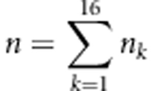be the total number of all individuals. The likelihood function in a backcross is

However, the maximum likelihood estimate in equation (5) is complicated. Thus, the complete information that includes all 64 genotypes for four markers and two SDL was used to construct the likelihood function, which is expressed as

where p_kl and n_kl (k=1,…,16; l=1,…,4) are the expected frequency and the observed number for the kth marker genotype and the lth SDL genotype, respectively, and 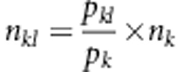. Theoretically, the Newtow–Raphson method may be used to obtain the maximum likelihood estimates in equation (6). Here, we adopt the expectation–maximisation (EM) algorithm (Dempster et al., 1977). The logarithm likelihood function is

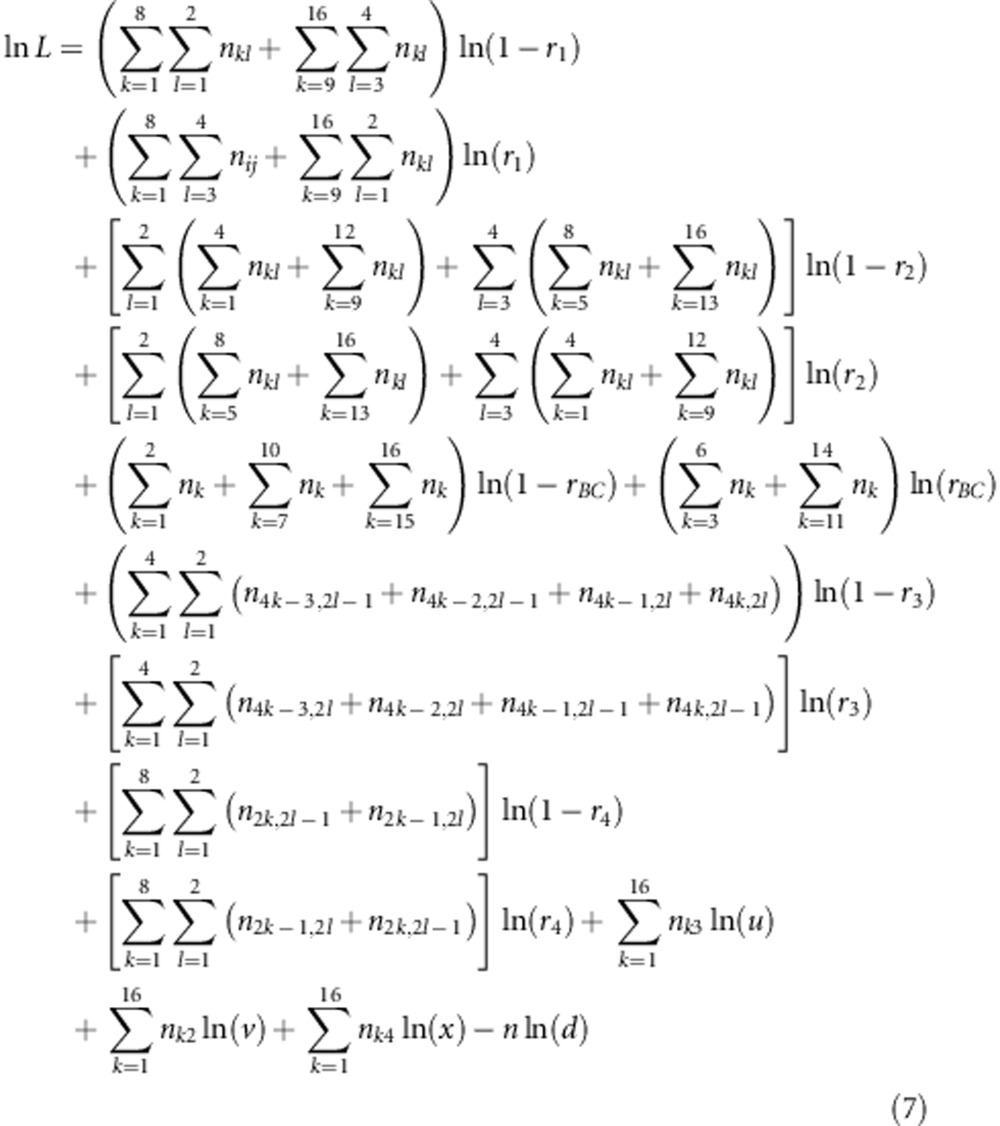where . The maximum likelihood estimate of each parameter is found by setting its partial derivative to zero and solving the equation to obtain

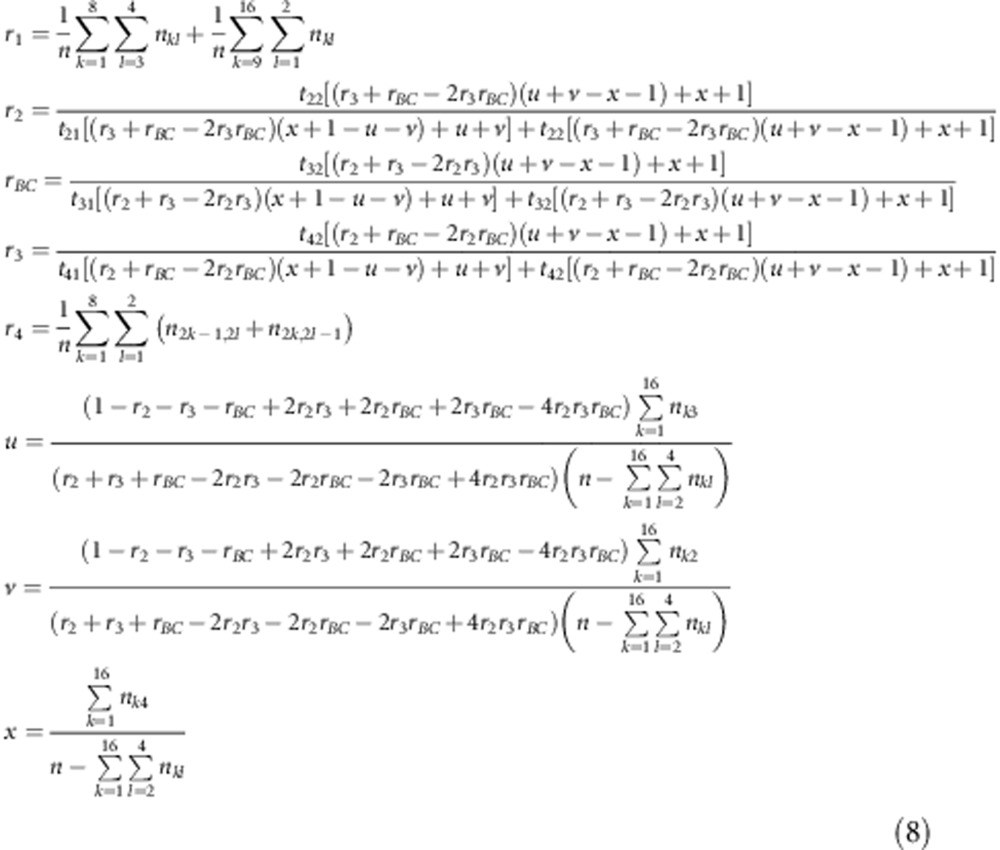where , , , , and . The estimates for r₁ and r₂ were used to correct the recombination fraction between markers A and B: r_AB=r₁+r₂−2r₁r₂; similarly, r_CD=r₃+r₄−2r₃r₄. When m markers are located in a linkage group, the number of estimates for r_AB is . Among these estimates, some may be overestimated and some may be underestimated; in this study, the median is our suggested estimate, which is validated by Monte Carlo simulation experiments. Although only selection parameters u, v and x were estimated, these parameters in the fitness model can be transferred to those in the liability model using equation (4). Therefore, only the estimates of parameters in the fitness model are given in this study.

Variance of recombination fraction

The expected Fisher's information score of the recombination fraction is given by

Where ln L=(n_AB+n_ab)ln(1−r)+(n_Ab+n_aB)ln r+n_Ab ln v+n_aB ln u+n_ab ln x−n ln[(1−r)(x+1)+r(u+v)]. For large samples, the variance of r was estimated by

Genetic model under zygotic selection in the F ₂ population

Liability model

The liability z_j of the jth F₂ individual under study could be described by the following model:

where a_k and d_k are the additive and dominant effects of the kth SDL (k=1, 2), respectively; i, j₁₂, j₂₁ and l are the additive-by-additive, additive-by-dominant, dominant-by-additive and dominant-by-dominant interaction effects of the two SDL, respectively; x_j.. is the dummy variable defined as x_jk1=1 and x_jk2=0 for SDL homozygote SS, x_jk1=0 and x_jk2=1 for SDL heterozygote Ss and x_jk1=−1 and x_jk2=0 for SDL homozygote ss (k=1, 2); and the other variables are similar to those in model (1). As nine possible genotypes for two linked SDL exist, the relative fitness f_l (l=1,…,9) can be easily calculated, and both the results and the expected frequencies are listed in Table 3.

Table 3. Expected frequencies of the nine genotypes under zygotic and gametic selection in the F₂ population.

Genotype	Relative fitness fl	Zygotic selection		Gametic selection
		in fitness model	in liability model	in fitness model	in liability model
S1S1S2S2	Φ(a1+a2+i)	(1−r2)/D1	(1−r)2 f1/d1	(1−r)2/D2	(1−r)2 f1/d2
S1S1S2s2	Φ(a1+d2+j12)	2r(1−r)v2/D1	2r(1−r)f2/d1	r(1−r)(vg+1)/D2	r(1−r)(f1+f3)/d2
S1S1s2s2	Φ(a1−a2−i)	r2v1/D1	r2f3/d1	r2vg/D2	r2f3/d2
S1s1S2S2	Φ(d1+a2+j21)	2r(1−r)u2/D1	2r(1−r)f4/d1	r(1−r)(ug+1)/D2	r(1−r)(f1+f2)/d2
S1s1S2s2	Φ(d1+d2+l)	2(1−2r+2r2)x4/D1	2(1−2r+2r2)f5/d1	[(1−r)2(xg+1)+r2(ug+vg)]/D2	[(1−r)2(f1+f9)+r2(f3+f7)]/d2
S1s1s2s2	Φ(d1−a2−j21)	2r(1−r)x3/D1	2r(1−r)f6/d1	r(1−r)(vg+xg)/D2	r(1−r)(f3+f7)/d2
s1s1S2S2	Φ(−a1+a2−i)	r2u1/D1	r2f7/d1	r2ug/D2	r2f7/d2
s1s1S2s2	Φ(−a1+d2−j12)	2r(1−r)x2/D1	2r(1−r)f8/d1	r(1−r)(ug+xg)/D2	r(1−r)(f7+f9)/d2
s1s1s2s2	Φ(−a1−a2+i)	(1−r)2x1/D1	(1−r)2f9/d1	(1−r)2xg/D2	(1−r)2 f9/d2

D₁=(1−r)²(x₁+1)+2r(1−r)(u₂+v₂+x₂+x₃)+r²(u₁+v₁)+2(1−2r+2r²)x₄.

D₂=2(1−r)(x_g+1)+2r(u_g+v_g).

d₁=(1−r)²(f₁+f₉)+2r(1−r)(f₂+f₄+f₆+f₈)+r² f₃+2(1−2r+2r²)f₅.

d₂=2(1−r)(f₁+f₉)+2r(f₃+f₇).

Fitness model

Two SDL under study are linked with a recombination fraction of r. In zygotic selection, the viabilities of S₁S₁S₂s₂, S₁S₁s₂s₂, S₁s₁S₂S₂, S₁s₁S₂s₂, S₁s₁s₂s₂, s₁s₁S₂S₂, s₁s₁S₂s₂ and s₁s₁s₂s₂ relative to S₁S₁S₂S₂ are assumed to be v₂, v₁, u₂, x₄, x₃, u₁, x₂ and x₁, respectively. Their expected frequencies (l=1,…,9) are also listed in Table 3.

Relationship between parameters in the above two models

The expected frequencies of one genotype under the liability and fitness models should be the same, that is, (l=1,…,9). Therefore, the relationship between parameters in the two models can be expressed as

Genetic model under gametic selection in the F ₂ population

Liability model

The genetic model under gametic selection is the same as model (11). Assume that female gametes and their mating processes are normal, that is, the frequencies of female gametes S₁S₂, S₁s₂, s₁S₂ and s₁s₂ are (1−r)/2, r/2, r/2 and (1−r)/2, respectively. If the marker segregation ratio shows deviation from the Mendelian ratio, the distortion is derived from the male gametes of an F₁ plant. Note that the frequencies of the nine genotypes under gamete selection are same as those under zygotic selection and that genotypes S₁S₁S₂S₂, S₁S₁s₂s₂, s₁s₁S₂S₂ and s₁s₁s₂s₂ are uniquely derived from the crosses S₁S₂/S₁S₂, S₁s₂/S₁s₂, s₁S₂/s₁S₂ and s₁s₂/s₁s₂, respectively. Thus, the frequencies of male gametes S₁S₂, S₁s₂, s₁S₂ and s₁s₂ are 2(1−r)f₁/d₁, 2rf₃/d₁, 2rf₇/d₁ and 2(1−r)f₉/d₁, respectively, and the expected frequencies of the nine genotypes in F₂ can be calculated as in Supplementary Table S1 (listed in Table 3). If we compare columns 4 and 6 in Table 3, the following equations can be found: 2f₂=f₁+f₃, 2f₄=f₁+f₇, 2f₆=f₃+f₉, 2f₈=f₇+f₉ and 2f₅=f₁+f₉=f₃+f₇.

Fitness model

Let the viabilities of male gametes S₁s₂, s₁S₂ and s₁s₂ relative to S₁S₂ be v_g, u_g and x_g, respectively. The expected frequencies of the nine genotypes under gametic selection are listed in Table 3.

Relationship between parameters in the above two models

The expected frequencies of one genotype under the liability and fitness models should be the same, that is, (l=1,…,9). The relationship between parameters in the two models can be expressed as

which is the same as equation (4) in the backcross. In fact, this relationship is reasonable. Under the situation of gametic selection, selection occurs during the gamete production stage but not the mating process. As we know, these gametes are formed in the F₁ plant stage, which is similar to a backcross.

Likelihood function and parameter estimation in the F ₂ population

If p_l and n_l (l=1,…,9) are the expected frequencies and observed number of the kth genotype for the two SDL, and 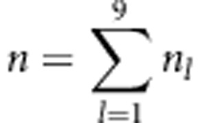is the total number of individuals, then the general likelihood function in F₂ can be expressed as

where p_l is under gametic selection or under zygotic selection.

Parameter estimation under zygotic selection

The genotypes of an SDL are unobserved if the SDL does not reside at the marker position. As described in a backcross, the information for four markers flanking with the two SDL can be used to estimate all of the parameters. However, there are 4096 (64 × 64) gamete combinations and 729 genotypes for four markers and two SDL. Using this calculation, it is time consuming to estimate the parameters. To reduce the running time, the information for three markers (A, B and C) flanking with the two SDL (S1 and S2) is utilised. The order of these loci are A, S₁, B, S₂ and C, and the recombination fractions for the four linked intervals are r₁, r₂, r₃ and r₄, respectively. There are 27 genotypes (observed) for three markers and nine genotypes (unobserved) for the two SDL. Thus, the complete information likelihood function is

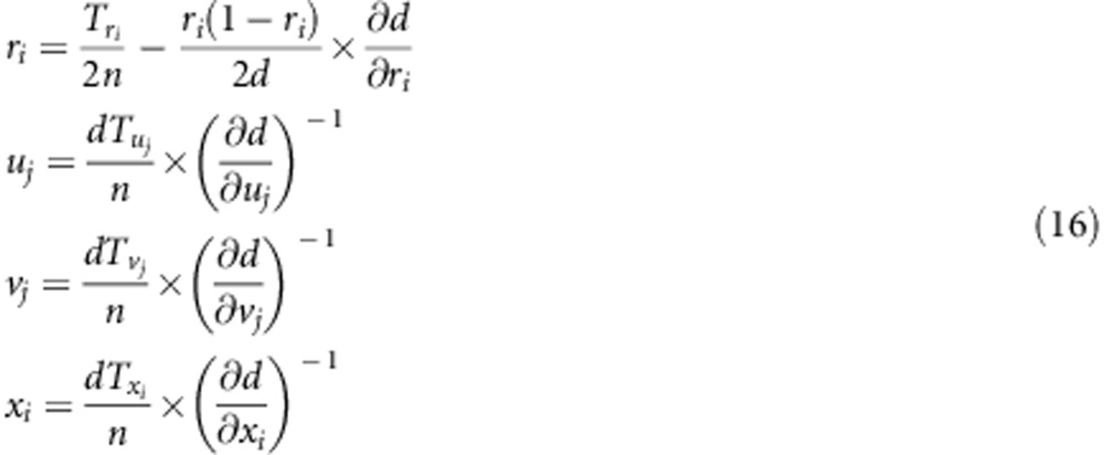
where p_kl and n_kl (k=1,…,27; l=1,…,9) are the expected frequencies and observed numbers of the kth marker genotype and the lth SDL genotype, respectively. The logarithm likelihood function and the partial derivative for each parameter are given in Supplementary Material A. The estimations of the parameters are

where d, , , , and (i=1,2,3,4; j=1,2) are listed in Supplementary File zygotic.xls. The estimates for r₁ and r₂ are used to estimate the recombination fraction between markers A and B: r_AB=r₁+r₂−2r₁r₂, which is the corrected recombinant fraction. When m markers are located in a linkage group, the number of estimates for r_AB is m−2. Similarly, the median is the suggested estimate.

Parameter estimation under gametic selection

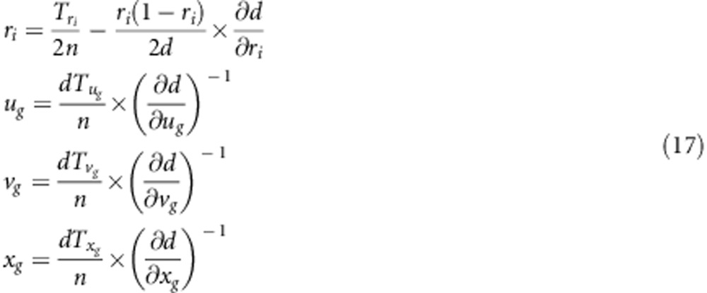
Four parameters, r, u_g, v_g and x_g, under gametic selection need to be estimated. The procedures and algorithm for the parameter estimation are similar to those under zygotic selection. Similarly, we obtain

where d, (i=1,2,3,4), , and are listed in Supplementary File gametic.xls. The strategy for estimate of r is the same as that under zygotic selection.

Variance of recombination fraction

The variances of recombination fraction r under gametic and zygotic selection in the F₂ population are

respectively, where K=2r(u₁+v₁+x₁+1)+2(2r−1)(2x₄−u₂−v₂−x₂−x₃)−2(x₁+1) and D=(1−r)²(x+1)+2r(1−r)(u₂+v₂+x₂+x₃)+r²(u₁+v₁)+2(1−2r+2r²)x₄.

Detection of selection type in the F ₂ population

The χ²-test of Pham et al. (1990) is used to determine whether the numbers of AA, Aa and aa genotypes in F₂, n_AA, n_Aa and n_aa follow the Mendelian segregation ratio of 1: 2: 1

If the test is significant, selection exists. To further clarify the selection type (that is, gametic vs zygotic), Lorieux et al. (1995b) suggest two χ² tests,

where is the allelic frequency of A in F₂. Gametic selection occurs if but not is significant; zygotic selection occurs if is significant (Lorieux et al., 1995b).

Statistical properties

At present, there are three approaches available. The first is the method that does not consider the effect of distorted markers, named method I, implemented by MapMaker v3.0 (Lander et al., 1987) or JoinMap v4.0. The second is the method that considers the effect of distorted markers, named method II (Lorieux et al., 1995a, 1995b; Zhu et al., 2007). The third is the new method described in this study, which considers the effect of epistatic distorted markers. Compared with methods I and II, some properties of the new method in a backcross population are summarised below:

1. The new method is equal to method I when u=v=x=1, and the new method is equal to method II when u≠1, v≠1 and x=1. This finding means that the new method is general and that methods I and II are specific.

2. An unbiased estimate for the recombinant fraction can be obtained when x+1=u+v or for method I; x=uv or for method II; and for all situations for the new method.

3. The overestimate for the recombinant fraction occurs when or u+v>x+1 for method I and or uv>x for method II. The underestimate for the recombinant fraction occurs when or u+v<x+1 for method I and or uv<x for method II.

4. Two linked SDL affect the estimates of the recombinant fraction for all marker intervals within the two linked SDL. The evidence is shown in Supplementary Material B.

5. The variance of recombinant fraction r for the new method is equal to and less than that for method I when u+v=x+1 and u+v<x+1, respectively. If u+v>x+1, two situations occur: the variance of r for the new method is greater and less than that for method I when and , respectively. The evidence is shown in Supplementary Material C.

Results

Monte Carlo simulation

Effect of heritability, marker interval length and sample size on the estimate of map distance

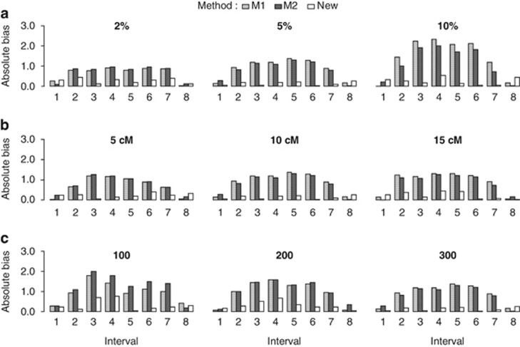
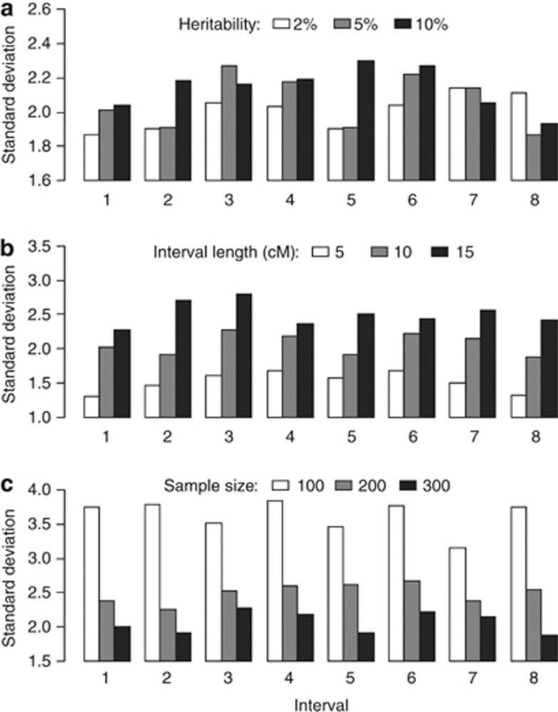
Nine equally spaced markers were simulated on a single-chromosome segment in a backcross population. Two SDL were placed at the middle of the second and seventh marker intervals. Three levels were set up for each factor in Monte Carlo simulated experiments: (1) SDL heritability, 2, 5 and 10% (2) interval length between adjacent markers, 5, 10 and 15 cM; and (3) sample size, 100, 200 and 300. All of the simulated parameters are shown in Supplementary Table S2. For each parameter combination, 200 replicated experiments were conducted, and the absolute bias and s.d. among the estimates from the 200 replicates were used to estimate the precision. All of the results for the backcross population are listed in Figures 1 and 2. The results showed that all of the estimates from the new method were unbiased (Figure 1). The two linked SDL do not affect the estimates of the map distances for marker intervals 1 and 8 (outside the two SDL) but do affect the estimates of the map distances for marker intervals 2–7 (within the two SDL) when methods I and II are adopted (Figure 1). In addition, the absolute bias and s.d. of the new method increase as the SDL heritability and marker interval length increase, and they decrease as the sample size increases (Figures 1 and 2). Similar results are also observed in F₂ (Supplementary Figures S1 and S2).

Figure 1.

Effect of SDL heritability (a), interval length (b) and sample size (c) on the estimate of map distance in a backcross population. (a) Interval length, 10 cM; sample size, 300; (b) SDL heritability, 5% sample size, 300; and (c) SDL heritability, 5% interval length, 10 cM.

Figure 2.

Effect of SDL heritability (a), interval length (b) and sample size (c) on the s.d. of the estimates from the new method in a backcross population. (a) Interval length, 10 cM; sample size, 300; (b) SDL heritability, 5% sample size, 300; and (c) SDL heritability, 5% interval length, 10 cM.

Effect of the SDL genetic model on linkage map construction

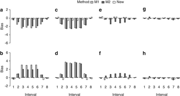
Eight genetic modes of SDL, listed in Figure 3 and Supplementary Table S3, were set up to investigate the effect of the SDL genetic model on the map distance under the liability and fitness models. The sample size was 300, and the marker interval length was 10 cM. The other parameters were the same as those in the above simulated experiment. All the results in the backcross are listed in Figure 3. The results were as follows: (1) all the estimates from the new method were unbiased. (2) Using method I, the estimates under SDL genetic modes 5–8 were unbiased because and u+v=x+1 (Figures 3e–h, and Supplementary Table S3); the estimates under SDL genetic modes 1 and 3 were underestimated because and u+v<x+1 (Figures 3a and c, and Supplementary Table S3); and the estimates under SDL genetic modes 2 and 4 were overestimated because and u+v>x+1 (Figures 3b and d, and Supplementary Table S3). Using method II, the estimates under SDL genetic modes 7 and 8 were unbiased because and uv=x (Figures 3g and h, and Supplementary Table S3); the estimates under SDL genetic modes 1, 3 and 5 were underestimated because and uv>x (Figures 3a, c and e, and Supplementary Table S3); and the estimates under SDL genetic modes 2, 4 and 6 were overestimated because and uv>x (Figures 3b, d and f, and Supplementary Table S3). (3) The bias was proportional to the above related size difference. For example, the bias of the estimates from method I in Figure 3d is larger than that in Figure 3b because in Figure 3d is larger than 0.62 in Figure 3b.

Figure 3.

Effect of SDL genetic mode on the estimate of map distance in a backcross population. The SDL parameters are as follows: (a) a₁=a₂=i=0.5; (b) a₁=−a₂=−i=0.5; (c) a₁=a₂=0,i=0.5; (d) a₁=a₂=0,i=−0.5; (e) a₁=−a₂=0,i=0.5; (f) a₁=a₂=0.5,i=0; (g) a₁=−0.5,a₂=i=0; and (h) a₁=0.5,a₂=i=0. The relationship among the parameters in the liability and fitness models is shown in Supplementary Table S3: and u+v<x+1 (a, c); and u+v>x+1 (b, d); and u+v=x+1 (e–h); and uv<x (a, c, e); and uv>x (b, d, f); and uv=x (g and h).

Effect of selection type in the F₂ population on linkage map construction

Gametic and zygotic selections of SDL in the F₂ population were simulated to investigate the effect of the selection type on map distance. SDL heritability was set at 5%, sample size was 300 and marker interval length was 10 cM. The other parameters were the same as those in the first simulated experiment. All of the data sets were first analysed by the χ²-test to determine the selection type. The results are listed in Table 4 and are consistent with the theoretical results. Each data set was then analysed twice: once under gametic selection and once under zygotic selection. The purpose was to determine which method was better in the case of inconsistent selection types of adjacent markers. The results are listed in Table 5. The results showed that new method works well under consistent selection types of adjacent markers. If gametic selection occurs at the ith locus and zygotic selection occurs at the (i+1)th locus, how to select the method for parameter estimation was unclear. As a result, the absolute bias under zygotic selection is less than that under gametic selection. Therefore, we recommend the zygotic selection approach to address this case.

Table 4. χ²-tests for marker segregation distortion, and gametic and zygotic selection.

Marker	χ2 for marker segregation distortion		for gametic selection		for zygotic selection
	Gametic selection	Zygotic selection	Gametic selection	Zygotic selection	Gametic selection	Zygotic selection
1	11.65**(6.35)	13.65**(6.29)	5.31* (3.10)	5.78*(3.05)	1.10(1.47)	2.99(3.41)
2	16.57**(7.32)	21.83**(7.54)	7.78**(3.59)	8.77**(3.79)	1.25(1.63)	6.71*(4.62)
3	18.93**(8.48)	23.60**(7.76)	8.93**(4.03)	9.85**(3.83)	1.36(1.65)	6.59*(4.63)
4	16.59**(7.78)	19.54**(7.68)	7.80**(3.74)	8.69**(3.71)	1.15(1.43)	3.67(3.92)
5	16.02**(7.47)	18.54**(7.34)	7.55**(3.59)	8.30**(3.64)	1.06(1.41)	3.18(3.51)
6	16.03**(6.88)	19.33**(7.21)	7.50**(3.33)	8.60**(3.69)	1.24(1.58)	3.57(3.33)
7	18.58**(7.79)	23.53**(7.27)	8.77**(3.72)	9.76**(3.69)	1.27(1.68)	6.62*(4.65)
8	16.83**(7.74)	21.14**(7.13)	7.90**(3.77)	8.49**(3.47)	1.18(1.56)	6.51*(4.55)
9	11.95**(6.39)	13.61**(5.93)	5.43*(3.15)	5.65*(2.81)	1.14(1.80)	3.25(3.15)

* and **: significances at the 0.05 and 0.01 levels, respectively. The s.d. among 200 replicates are in parentheses.

Table 5. Comparison of the gametic and zygotic model methods under gametic and zygotic selection in the F₂ population.

Selection type	Method	Marker interval
		1	2	3	4	5	6	7	8
Gametic	gm	9.96(1.34)	10.08(1.29)	9.88(1.31)	9.79(1.26)	9.93(1.33)	9.88(1.33)	9.97(1.33)	9.90(1.39)
	zm	9.92(1.33)	9.59(1.18)	9.41(1.20)	9.33(1.16)	9.47(1.22)	9.41(1.21)	9.49(1.21)	9.85(1.38)
Zygotic	gm	10.35(1.49)	12.67(2.10)	11.83(1.99)	11.94(2.22)	12.13(1.87)	11.88(1.89)	12.81(2.26)	10.25(1.54)
	zm	10.05(1.41)	10.01(1.39)	9.50(1.30)	9.59(1.46)	9.71(1.25)	9.50(1.27)	10.08(1.52)	9.96(1.47)

Abbreviations: gm, gametic model method, zm: zygotic model method. Marker interval length, 10 cM.

Real data analysis in rice

To further demonstrate the new method, a real data set for a backcross population (Oryza sativa/Oryza longistaminata//O. sativa) (Causse et al., 1994) was downloaded from the McCouch RiceLab website (http://ricelab.plbr.cornell.edu/Causse_at_al_1994) and re-analysed. The data set is composed of 617 markers on 12 chromosomes. On the basis of 12 linkage groups constructed by Mapdisto v1.7.7 (Lorieux, 2012), all of the map distances between flanking markers were corrected by software package DistortedMap of the new method (Supplementary file DistortedMap). All of the results are listed in Supplementary Table S4 and Supplementary Figure S3. To further illustrate the new method, all of the map distances on chromosome 3, with several severely distorted segregation regions, were calculated by methods I, II and new (Table 6). As a result, in regions with normal Mendelian segregation, the estimates of the recombinant fraction by the above three methods were similar, such as for markers CDO375, RCH and RZ696, and almost all the estimates for u, v and x were closer to 1 than those in regions with distorted segregation. In the distorted segregation region between markers RZ585 and RZ284, the χ²-test for marker RZ284 was significant (χ²=18.60, P=1.61e−5), and the map distances of 4.75 and 5.29 cM, calculated by methods I and II, respectively, were less than 6.52 cM, calculated by the new method, indicating that the results from methods I and II were underestimates because u+v=0.93<x+1=1.30 for method I and uv=0.19<x=0.30 for method II.

Table 6. Comparison of the map distances on chromosome 3 from methods I, II and the new method in a rice data analysis.

Marker	χ2	Selection	Map distances (cM) from various methods			Segregation distortion loci effect
			I	II	New	u	v	x
RZ497	3.57	No	—	—	—	—	—	—
RZ25	10.89**	Gametic/zygotic (g/z)	1.14	0.15	0.15	11.45	0.05	0.53
RZ22	11.56**	g/z	0.00	0.00	0.00	0.71	0.71	0.50
RZ18	5.38*	g/z	1.17	0.17	1.26	0.01	1.43	0.55
CDO375	0.29	No	0.00	0.00	0.00	0.84	0.84	0.71
RCH	1.90	No	8.95	8.99	8.95	0.91	0.91	0.82
RZ696	1.08	No	9.76	9.81	9.76	0.73	0.97	0.69
RZ394	4.57*	g/z	2.80	0.68	0.68	7.07	0.10	0.71
RZ452	3.85*	g/z	0.00	0.00	0.00	0.80	0.80	0.65
RZ251	3.32	No	1.22	0.23	0.23	9.34	0.08	0.73
RZ585	8.89**	g/z	2.80	0.49	0.49	8.58	0.06	0.49
RZ284	18.6**	g/z	4.75	5.29	6.52	0.62	0.31	0.30
RZ672	12.49**	g/z	3.07	3.48	4.70	0.44	0.43	0.36
CDO938	8.05**	g/z	3.10	3.26	5.26	0.44	0.44	0.52
RG745	8.78**	g/z	0.00	0.00	0.00	0.75	0.75	0.56
RZ574	6.37*	g/z	0.00	0.00	0.00	0.79	0.79	0.63
RZ1000	12.52**	g/z	1.65	0.28	2.44	1.04	0.01	0.56
CDO608	4.74*	g/z	2.03	0.53	2.46	0.02	1.32	0.63
RG227	3.08	No	0.00	0.00	0.00	0.77	0.77	0.59
RZ678	11.12**	g/z	0.00	0.00	0.00	0.85	0.85	0.72
BCD734	11.56**	g/z	0.00	0.00	0.00	0.72	0.72	0.52
BCD1092	8.38**	g/z	0.00	0.00	0.00	0.72	0.72	0.52
CD1053X	13.79**	g/z	0.00	0.00	0.00	0.73	0.73	0.53
RZ399	7.19**	g/z	0.00	0.00	0.00	0.73	0.73	0.53
RZ517	12.3**	g/z	0.00	0.00	0.00	0.74	0.74	0.55
RZ16	10.12**	g/z	0.00	0.00	0.00	0.70	0.70	0.49
CDO260	16.64**	g/z	0.00	0.00	0.00	0.69	0.69	0.48
CDO33X	12.96**	g/z	0.00	0.00	0.00	0.67	0.67	0.44
RG191	9.24**	g/z	1.24	0.36	2.28	0.80	0.02	0.52
RG224	3.96*	g/z	0.00	0.00	0.00	0.78	0.78	0.61
CD1387B	12.96**	g/z	0.00	0.00	0.00	0.85	0.85	0.72
CDO1395	13.5**	g/z	0.00	0.00	0.00	0.68	0.68	0.46
RZ313	11.71**	g/z	0.00	0.00	0.00	0.69	0.69	0.48
RG450	15.36**	g/z	0.00	0.00	0.00	0.69	0.69	0.47
RG369A	11.33**	g/z	3.30	3.34	4.63	0.34	0.69	0.47
RG100	10.13**	g/z	2.65	0.50	3.95	0.99	0.01	0.51
RZ545	4.76*	g/z	0.00	0.00	0.00	0.72	0.72	0.51
RZ742B	5.45*	g/z	4.66	4.54	5.16	0.47	0.96	0.59
CDO1069	14.44**	g/z	3.38	0.34	5.29	0.91	0.00	0.46
RZ993X	12.63**	g/z	2.29	2.49	3.52	0.46	0.45	0.43
RZ891	7.51**	g/z	2.29	0.30	3.03	0.00	1.13	0.51
RZ987	5.76*	g/z	2.52	0.45	3.10	1.30	0.01	0.62
RZ329	8.49**	g/z	2.49	2.57	2.56	0.77	0.79	0.60
RG944	8.38**	g/z	7.57	7.55	8.00	0.48	0.95	0.51
RG348	9.91**	g/z	6.83	5.93	6.91	1.16	0.29	0.47
RG104	2.85	No	5.69	5.11	5.11	0.46	1.36	0.63
CDO20	14.82**	g/z	7.64	6.92	6.92	1.31	0.44	0.58
CDO481	5.31*	g/z	22.82	23.62	25.97	0.37	0.82	0.37
RG432	2.47	No	27.10	18.80	18.80	0.37	2.56	0.96

* and **: significances at the 0.05 and 0.01 levels, respectively.

Discussion

Although the new method proposed for linkage map correction in this study is based on the epistatic genetic model of SDL, it is suitable not only for the above model but also for normal (Supplementary Table S5) and distorted (Figure 3) markers. When no SDL is identified in a linkage group, the estimates for map distances by the above three approaches are almost unbiased and close to the true values (Supplementary Table S5). We also calculated the s.d. of the estimates by two approaches: one using Fisher's information (SD1) and the other using the variation of the estimates across 200 replicates (SD2). For the former, similar results were observed across the above three methods; for the latter, slightly increased results were found from method I to II and from method II to the new method (Supplementary Table S5). These findings are reasonable because the number of parameters gradually increased in the above three methods, and the accumulated errors from their corresponding estimates were also increased. If multi-SDL are considered in a linkage group, the corrected results for the genetic distance are more accurate using the new method than using methods I and II (Supplementary Table S5). However, SD1 and SD2 are slightly larger for the new method than for methods I and II. The theoretical evidence is given in Supplementary Material C.

With respect to statistical properties 2 and 3 in the backcross, the evidence exists. Using method I, the recombinant fraction is estimated by 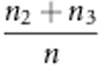. If the expectations of n₂, n₃ and n in the liability and fitness models are used to estimate n₂, n₃ and n, respectively, the two properties can be demonstrated. In the liability model, . If , then , which is an unbiased estimate; if , then , an overestimate; and if , then , an underestimate. In the fitness model, . By using a similar approach, the statistical properties 2 and 3 can be obtained. Using method II, the recombinant fraction is estimated by 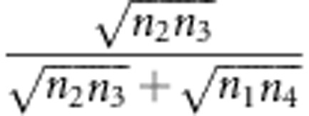(Lorieux et al., 1995a). In the fitness model, the estimate is changed to . If uv=x, then , which is an unbiased estimate; if uv>x, then , an overestimate; and if uv<x, then , an underestimate. In the liability model, 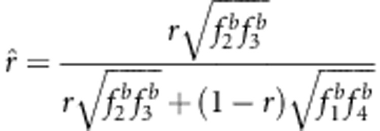. By using a similar approach, the statistical properties 2 and 3 can also be obtained. These properties have been confirmed by the Monte Carlo simulation studies and real data analysis in this study.

If two SDL of one SDL-by-SDL interaction are placed in the same linkage group, this interaction does not affect the estimate of the recombinant fraction outside the SDL intervals. In Supplementary Material B, the estimates for the recombinant fractions outside the SDL intervals are obtained as R₁=(n_Ab+n_aB), R₂=(n_Bc+n_bC)/n, R₃=(n_De+n_dE)/n and R₄=(n_Ef+n_eF)/n. Obviously, the four estimates are independent of the viability parameters, which are evidence of the above result. Similar evidence was also observed in the Monte Carlo simulation studies. If two SDL of one SDL-by-SDL interaction are placed in different linkage groups, this interaction does not affect the estimates of the recombinant fraction. In Supplementary Material B, the estimates for the two recombinant fractions involved this interaction are obtained as 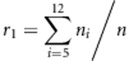and 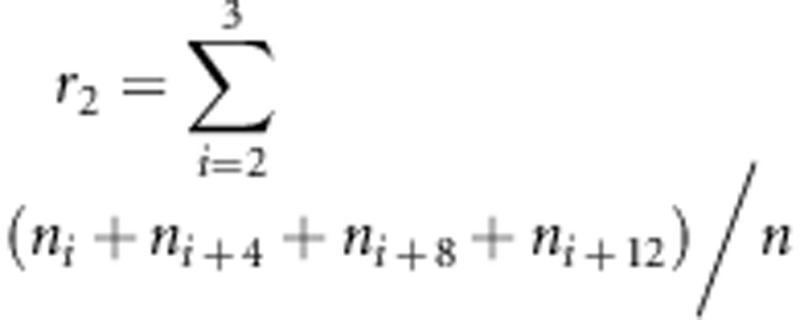. Obviously, the two estimates for both r₁ and r₂ are independent of the viability parameters, representing evidence of the above result. In addition, the results in Figures 2g and h showed that the estimate for the recombination fraction is unaffected by the distorted markers due to only one SDL in one linkage group. This finding is consistent with the previous results in Bailey (1949), Lorieux et al. (1995a, 1995b) and Zhu et al. (2007).

In linkage group construction, some multi-point approaches are widely used. Among these approaches, Lander and Green (1987) first proposed a Markov chain multi-point approach to utilise missing markers. Jiang and Zeng (1997) then extended the method of Lander and Green (1987) to address dominant and missing markers, and Zhu et al. (2007) further extended the multi-point method to address distorted, dominant and missing markers. In this study, epistatic distorted markers are also considered as well. In fact, once the transition probability matrix H(r) from markers A to B is determined, the multi-point method including epistatic distorted markers should work well. Here, we provide these matrices as follows:

for a backcross population,

for the gametic selection approach in F₂, and

for the zygotic selection approach in F₂.

In animal and plant genetics, epistasis for viability selection has been detected in the studies of Chang and Noor (2010), Li et al. (2011) and Kubo et al. (2008). Thus, the method in this study should be developed. This method may be extended to additional biparental populations, for example, recombination inbred lines. The new method deals only with recombinant fraction correction, not with linkage group construction. With respect to this construction, the Mapmaker, Mapmanager, Joinmap and Mapdisto programs are available. Once linkage groups have been constructed and distorted markers exist, the new method can be used to correct bias.

Data archiving

All simulated datasets are available from the public website: http://jpkc.njau.edu.cn/swtj/show.asp?classid=44&classtype=26. The real dataset can be retrieved from: http://ricelab.plbr.cornell.edu/Causse_at_al_1994.

The authors declare no conflict of interest.

References

- Alheit KV, Reif JC, Maurer HP, Hahn V, Weissmann EA, Miedaner T, et al. Detection of segregation distortion loci in triticale (x triticosecale Wittmack) based on a high-density DArT marker consensus genetic linkage map. BMC Genomics. 2011;12:380. doi: 10.1186/1471-2164-12-380. [DOI] [PMC free article] [PubMed] [Google Scholar]
- Bailey NTJ. The estimation of linkage with differential viability, II and III. Heredity. 1949;3:220–228. doi: 10.1038/hdy.1949.13. [DOI] [PubMed] [Google Scholar]
- Barchi L, Lanteri S, Portis E, Stàgel A, Valè G, Toppino L, et al. Segregation distortion and linkage analysis in eggplant (Solanum melongena L.) Genome. 2010;53:805–815. doi: 10.1139/g10-073. [DOI] [PubMed] [Google Scholar]
- Bomblies K, Lempe J, Epple P, Warthmann N, Lanz C, Dangl JL, et al. Autoimmune response as a mechanism for a Dobzhansky-Muller-type incompatibility syndrome in plants. PLoS Biol. 2007;5:1962–1972. doi: 10.1371/journal.pbio.0050236. [DOI] [PMC free article] [PubMed] [Google Scholar]
- Brummer EC, Bouton JH, Kochert G. Development of an RFLP map in diploid alfalfa. Theor Appl Genet. 1993;86:329–332. doi: 10.1007/BF00222097. [DOI] [PubMed] [Google Scholar]
- Causse MA, Fulton TM, Cho YG, Ahn SN, Chunwongse J, Wu K, et al. Saturated molecular map of the rice genome based on an interspecific backcross population. Genetics. 1994;138:1251–1274. doi: 10.1093/genetics/138.4.1251. [DOI] [PMC free article] [PubMed] [Google Scholar]
- Chang AS, Noor MAF. Epistasis modifies the dominance of loci causing hybrid male sterility in the drosophila pseudoobscura species group. Evolution. 2010;64:253–260. doi: 10.1111/j.1558-5646.2009.00823.x. [DOI] [PMC free article] [PubMed] [Google Scholar]
- Cloutier S, Cappadocia M, Landry BS. Analysis of RFLP mapping inaccuracy in Brassica napus L. Theor Appl Genet. 1997;95:83–91. doi: 10.1007/BF00223890. [DOI] [PubMed] [Google Scholar]
- Dempster AP, Laird NM, Rubin DB. Maximum likelihood from incomplete data via the EM algorithm. J R Stat Soc B. 1977;39:1–38. [Google Scholar]
- Dobzhansky T. Studies on hybrid sterility. II. Localization of sterility factors in Drosophila pseudoobscura hybrids. Genetics. 1936;21:113–135. doi: 10.1093/genetics/21.2.113. [DOI] [PMC free article] [PubMed] [Google Scholar]
- Faris JD, Laddomada B, Gill BS. Molecular mapping of segregation distortion loci in Aegilops tauschii. Genetics. 1998;49:319–327. doi: 10.1093/genetics/149.1.319. [DOI] [PMC free article] [PubMed] [Google Scholar]
- Jiang CJ, Zeng ZB. Mapping quantitative trait loci with dominant and missing markers in various crosses from two inbred lines. Genetica. 1997;101:47–56. doi: 10.1023/a:1018394410659. [DOI] [PubMed] [Google Scholar]
- Kaló P, Endre G, Zimányi L, Csanádi G. Construction of an improved linkage map of diploid alfalfa (Medicago sativa) Theor Appl Genet. 2000;100:641–657. [Google Scholar]
- Kreike DD, Stiekema WJ. Reduced recombination and distorted segregation in a Solanum tuberosum (2 × ) × S.spegazzinii (2 × ) hybrid. Genome. 1997;40:180–187. doi: 10.1139/g97-026. [DOI] [PubMed] [Google Scholar]
- Kubo T, Yamagata Y, Eguchi M, Yoshimura A. A novel epistatic interaction at two loci causing hybrid male sterility in an inter-subspecific cross of rice (Oryza sative L.) Genes Genet. Syst. 2008;83:443–453. doi: 10.1266/ggs.83.443. [DOI] [PubMed] [Google Scholar]
- Kärkkäinen K, Koski V, Savolainen O. Geographical variation in the inbreeding depression of Scots pine. Evolution. 1996;50:111–119. doi: 10.1111/j.1558-5646.1996.tb04477.x. [DOI] [PubMed] [Google Scholar]
- Lander ES, Green P. Construction of multilocus genetic linkage maps in humans. Proc Natl Acad Sci USA. 1987;84:2363–2367. doi: 10.1073/pnas.84.8.2363. [DOI] [PMC free article] [PubMed] [Google Scholar]
- Lander ES, Green P, Abrahamson J, Barlow A, Daly MJ, Lincoln SE, et al. MAPMAKER: an interactive computer package for constructing primary genetic linkage maps of experimental and natural populations. Genomics. 1987;1:174–181. doi: 10.1016/0888-7543(87)90010-3. [DOI] [PubMed] [Google Scholar]
- Lashermes P, Combes MC, Prakash NS, Trouslot P, Lorieux M, Charrier A. Genetic linkage map of Coffea canephora: Effect of segregation distortion and analysis of recombination rate in male and female meiosis. Genome. 2001;44:589–596. [PubMed] [Google Scholar]
- Leppälä J, Bokma F, Savolainen O. Investigating incipient speciation in Arabidopsis lyrata from patterns of transmission ratio distortion. Genetics. 2013;194:697–708. doi: 10.1534/genetics.113.152561. [DOI] [PMC free article] [PubMed] [Google Scholar]
- Li XH, Wang XJ, Wei YL, Brummer EC. Prevalence of segregation distortion in diploid alfalfa and its implications for genetics and breeding applications. Theor Appl Genet. 2011;123:667–679. doi: 10.1007/s00122-011-1617-5. [DOI] [PubMed] [Google Scholar]
- Lorieux M. MapDisto: fast and efficient computation of genetic linkage maps. Mol Breed. 2012;30:1231–1235. [Google Scholar]
- Lorieux M, Goffinet B, Perrier X, González-de-león D, Lanaud C. Maximum-likelihood models for mapping genetic markers showing segregation distortion. 1. Backcross population. Theor Appl Genet. 1995;90:73–80. doi: 10.1007/BF00220998. [DOI] [PubMed] [Google Scholar]
- Lorieux M, Perrier X, Goffinet B, Lanaud C, González-de-león D. Maximum-likelihood models for mapping genetic markers showing segregation distortion. 2. F2 populations. Theor Appl Genet. 1995;90:81–89. doi: 10.1007/BF00220999. [DOI] [PubMed] [Google Scholar]
- Lu H, Romero-Severson J, Bernardo R. Chromosomal regions associated with segregation distortion in maize. Theor Appl Genet. 2002;105:622–628. doi: 10.1007/s00122-002-0970-9. [DOI] [PubMed] [Google Scholar]
- Luo L, Zhang YM, Xu S. A quantitative genetics model for viability selection. Heredity. 2005;94:347–355. doi: 10.1038/sj.hdy.6800615. [DOI] [PubMed] [Google Scholar]
- Mangelsdorf PC, Jones DF. The expression of Mendelian factors in the gametophyte of maize. Genetics. 1926;11:423–455. doi: 10.1093/genetics/11.5.423. [DOI] [PMC free article] [PubMed] [Google Scholar]
- McCouch SR, Kochert G, Yu Z, Wang Z, Khush GS, Coffman WR, et al. Molecular mapping of rice chromosomes. Theor Appl Genet. 1988;76:815–829. doi: 10.1007/BF00273666. [DOI] [PubMed] [Google Scholar]
- McMullen MD, Kresovich S, Villeda HS, Bradbury P, Li H, Sun Q, et al. Genetic properties of the maize nested association mapping population. Science. 2009;325:737–740. doi: 10.1126/science.1174320. [DOI] [PubMed] [Google Scholar]
- Muller H. Isolating mechanisms, evolution, and temperature. Biol Symp. 1942;6:71–125. [Google Scholar]
- Paterson AH, Lander ES, Hewitt J, Peterson S, Lincoln SE. Resolution of quantitative traits into mendelian factors by using a complete map of restriction fragment length polymorphism. Nature. 1988;335:721–726. doi: 10.1038/335721a0. [DOI] [PubMed] [Google Scholar]
- Pham JL, Glaszmann JC, Sano R, Barbier P, Ghesquiere A, Second G. Isozyme markers in rice: genetic analysis and linkage relationships. Genome. 1990;33:348–359. [Google Scholar]
- Phillips PC. Epistasis—the essential role of gene interactions in the structure and evolution of genetic systems. Nat Rev Genet. 2008;9:855–867. doi: 10.1038/nrg2452. [DOI] [PMC free article] [PubMed] [Google Scholar]
- Rick CM. Abortion of male and female gametes in the tomato determined by allelic interaction. Genetics. 1966;53:85–96. doi: 10.1093/genetics/53.1.85. [DOI] [PMC free article] [PubMed] [Google Scholar]
- Sandler L, Hiraizumi Y, Sandler I. Meiotic drive in natural populations of Drosophila melanogaster. I. the cytogenetic basis of segregation-distortion. Genetics. 1959;44:233–250. doi: 10.1093/genetics/44.2.233. [DOI] [PMC free article] [PubMed] [Google Scholar]
- Törjék O, Witucka-Wall H, Meyer RC, Korff M, Kusterer B, Rautengarten C, et al. Segregation distortion in Arabidopsis C24/Col-0 and Col-0/C24 recombinant inbred line populations is due to reduced fertility caused by epistatic interaction of two loci. Theor Appl Genet. 2006;113:1551–1561. doi: 10.1007/s00122-006-0402-3. [DOI] [PubMed] [Google Scholar]
- Wang CM, Zhu CS, Zhai HQ, Wan JM. Mapping segregation distortion loci and quantitative trait loci for spikelet sterility in rice (Oryza sative L.) Genet Res. 2005;86:97–106. doi: 10.1017/S0016672305007779. [DOI] [PubMed] [Google Scholar]
- Xie SQ, Chen JG. A statistical method for genetic mapping of sterility genes that exhibit epistasis in remote hybridization of plants using molecular markers in an F2 population. Chin Sci Bull. 2012;57:2681–2687. [Google Scholar]
- Xu Y, Zhu L, Xiao L, Huang N, McCouch SR. Chromosomal regions associated with segregation distortion of molecular markers in F2, backcross, double haploid, and recombinant inbred populations in rice (Oryza sativa L.) Mol Gen Genet. 1997;253:535–545. doi: 10.1007/s004380050355. [DOI] [PubMed] [Google Scholar]
- Yang J, Zhao X, Cheng K, Du H, Ouyang Y, Chen J, et al. A killer-protector system regulates both hybrid sterility and segregation distortion in rice. Science. 2012;337:1336–1340. doi: 10.1126/science.1223702. [DOI] [PubMed] [Google Scholar]
- Zhu CS, Wang CM, Zhang YM. Modeling segregation distortion for viability selection I. Reconstruction of genetic linkage maps with distorted markers. Theor Appl Genet. 2007;114:295–305. doi: 10.1007/s00122-006-0432-x. [DOI] [PubMed] [Google Scholar]
Associated Data
This section collects any data citations, data availability statements, or supplementary materials included in this article.