Characterization of Tissue Histopathology via Predictive Sparse Decomposition and Spatial Pyramid Matching

Abstract

Image-based classification of tissue histology, in terms of different components (e.g., subtypes of aberrant phenotypic signatures), provides a set of indices for tumor composition. Subsequently, integration of these indices in whole slide images (WSI), from a large cohort, can provide predictive models of the clinical outcome. However, the performance of the existing histology-based classification techniques is hindered as a result of large technical and biological variations that are always present in a large cohort. In this paper, we propose an algorithm for classification of tissue histology based on predictive sparse decomposition (PSD) and spatial pyramid matching (SPM), which utilize sparse tissue morphometric signatures at various locations and scales. The method has been evaluated on two distinct datasets of different tumor types collected from The Cancer Genome Atlas (TCGA). The novelties of our approach are: (i) extensibility to different tumor types; (ii) robustness in the presence of wide technical and biological variations; and (iii) scalability with varying training sample size.

1 Introduction

Tissue sections are often stained with hematoxylin and eosin (H&E), which label DNA (e.g., nuclei) and protein contents, respectively, in various shades of color. They can provide a wealth of information about the tissue architecture. At macro level, tissue composition (e.g., stroma versus tumor) can be quantified. At micro level, cellular features such as cell types, cell state, and cellular organization can be queried. Aberrations in the tissue architecture often reflect disease progression. However, outcome-based analysis requires a large cohort, and the performance of the existing techniques is hindered as a result of large technical and biological variations that are always present in such a cohort.

In this paper, we propose a tissue classification method based on predictive sparse decomposition (PSD) [1] and spatial pyramid matching (SPM) [2], which utilize sparse tissue morphometric signatures at various locations and scales. Because of the robustness of unsupervised feature learning and the effectiveness of the SPM framework, our method achieves excellent performance even with small number of training samples across independent datasets of tumors. As a results, the composition of tissue histopathology in WSI can be characterized. Equally important, mix grading can also be quantified in terms of tumor composition. Computed compositional indices, from WSI, can then be utilized for outcome based analysis, i.e., survival, response to therapy.

Organization of this paper is as follows: Section 2 reviews related works. Sections 3 and 4 describes the details of our proposed method and experimental validation. Lastly, section 5 concludes the paper.

2 Related Work

For the analysis of the H&E stained sections, several excellent reviews can be found in [3,4]. Fundamentally, the trend has been based either on nuclear segmentation and corresponding morphometric representation [5,6], or patch-based representation of the histology sections [7,8]. The major challenge for tissue classification is the large amounts of technical and biological variations in the data, which typically results in techniques that are tumor type specific. To overcome this problem, recent studies have focused on either fine tuning human engineered features [7], or applying automatic feature learning [9,8], for robust representation.

In the context of image categorization research, the SPM kernel [2] has emerged as a major component for the state-of-art systems [10] for its effectiveness in practice.

Pathologists often use “context” to assess the disease state. At the same time, SPM partially captures context because of its hierarchical nature. Motivated by the works of [2,1], we encode sparse tissue morphometric signatures, at different locations and scales, within the SPM framework. The end results are highly robust and effective systems across multiple tumor types with limited number of training samples.

3 Approach

Proposed approach (PSDSPM) is shown in Figure 1, where the traditional SIFT is replaced with with sparse tissue morphometric feature, generated through unsupervised feature learning, within the SPM framework. It consists of the following steps:

1. Construct sparse auto encoder (W) for the extraction of sparse tissue morphometric feature by the following optimization:

   $$\underset{\mathbf{B},\mathbf{X},\mathbf{W}}{\min }\sum _{n=1}^N{\mid \mid {\mathbf{y}}_n-{\mathbf{x}}_n\mathbf{B}\mid \mid }_2^2+\lambda {\mid {\mathbf{x}}_n\mid }_1+{\mid \mid {\mathbf{x}}_n-{\mathbf{y}}_n\mathbf{W}\mid \mid }_2^2$$ (1)

   where Y = [y₁, …, y_N] is a set of vectorized image patches; B is a set of basis functions; X = [x₁, …, x_N] is a set of sparse tissue morphometric features; and W is the auto encoder. The training process is as follows:

   1. Randomly initialize B and W.
   2. Fix B and W and minimize Equation 1 with respect to X, where X for each input vector is estimated via the gradient descent method.
   3. Fix X and estimate B and W, where B and W are approximated through stochastic gradient descent algorithm.

   Examples of computed basis functions from the GBM and KIRC datasets are shown in Figure 2. It can be seen that the dictionary captures color and texture information in the data which are difficult to obtain using human engineered features.
2. Construct dictionary (D), where D = [d₁, …, d_K]^T are the K sparse tissue morphometric types to be learned by the following optimization:

   $$\begin{array}{cc}\hfill & \underset{\mathbf{D},\mathbf{Z}}{\min }\sum _{m=1}^M{\mid \mid {\mathbf{x}}_m-{\mathbf{z}}_m\mathbf{D}\mid \mid }^2\hfill \\ \hfill & \text{subject to}card\left({\mathbf{z}}_m\right)=1,\mid {\mathbf{z}}_m\mid =1,{\mathbf{z}}_m⪰0,\forall m\hfill \end{array}$$ (2)

   where X = [x₁, …, x_M]^T is a set of sparse tissue morphometric features generated through the auto-encoder (W); Z = [z₁, …, z_M]^T indicates the assignment of the sparse tissue morphometric type, card(z_m) is a cardinality constraint enforcing only one nonzero element of z_m, z_m ⪰ 0 is a non-negative constraint on the elements of z_m, and |z_m| is the L1-norm of z_m. During training, Equation 2 is optimized with respect to both Z and D; In the coding phase, for a new set of X, the learned D is applied, and Equation 2 is optimized with respect to Z only.
3. Construct spatial histogram for SPM [2]. This is done by repeatedly subdividing an image and computing the histograms of different sparse tissue morphometric types over the resulting subregions. As a result, the spatial histogram, H, is formed by concatenating the appropriately weighted histograms of all sparse tissue morphometric types at all resolutions,

   $$\begin{array}{cc}\hfill H_0=& H_0^0;H_l=(H_l^1,\dots ,H_l^{4^l}),1\le l\le L\hfill \\ \hfill H=& (\frac{1}{2^L}{H}_0,\frac{1}{2^L}{H}_1,\dots ,\frac{1}{2^{L-l+1}}{H}_l,\dots ,\frac{1}{2}{H}_L)\hfill \end{array}$$ (3)

   where (·) is the vector concatenation operator, l ∈ {0, …, L} is the resolution of the image pyramid, H_l is the concatenation of histograms for all image grids at certain resolution, l.

4. Transfer a χ² support vector machine (SVM) into a linear SVM based on a homogeneous kernel map [11]. In practice, the intersection kernel and χ² kernel have been found to be the most suitable for histogram representations [12]. In this step, a homogenous kernel map is applied to approximate the χ² kernel, which enables the efficiency by adopting learning methods for linear kernels, i.e., linear SVM.

5. Construct multi-class linear SVM for classification. In our implementation, the classifier is trained using the LIBLINEAR [13] package.

Fig. 1.

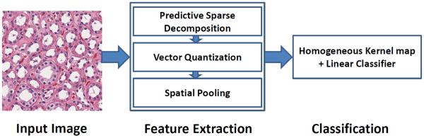
Computational steps of the proposed our approach (PSDSPM)

Fig. 2.

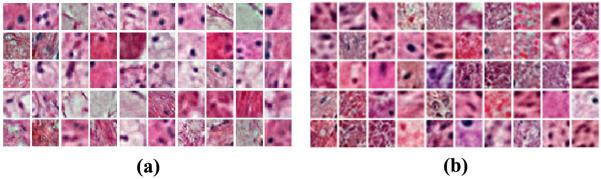
Representative set of basis functions, B, for a) the KIRC dataset, and b) the GBM dataset

4 Experiments and Discussion

We have evaluated four classification methods on two distinct datasets, curated from (i) Glioblastoma Multiforme (GBM) and (ii) Kidney Renal Clear Cell Carcinoma (KIRC) from TCGA, which are publicly available from the NIH (National Institute of Health) repository. The four methods are:

1. PSDSPM: the nonlinear kernel SPM that uses spatial-pyramid histograms of sparse tissue morphometric types;

2. PSD [1]: the sparse tissue morphometric features with max-pooling strategy, and RBF kernels;

3. ScSPM [12]: the linear SPM that uses linear kernel on spatial-pyramid pooling of SIFT sparse codes;

4. KSPM [2]: the nonlinear kernel SPM that uses spatial-pyramid histograms of SIFT features and χ² kernels;

In the implementation of ScSPM and KSPM, the dense SIFT features were extracted on 16 × 16 patches sampled from each image on a grid with step-size 8 pixels.

For both PSDSPM and PSD, we fixed the sparse constraint parameter λ to be 0.3, image patch size to be 20 × 20, and the number of basis functions to be 1024, empirically, to achieve the best performance. For ScSPM, we fixed the sparse constraint parameter λ to be 0.15, empirically, to achieve the best performance. For both PSDSPM and KSPM, we used standard K-means clustering for the construction of dictionary, where the elements was randomly initialized and iteratively refined in the Euclidean space. Additionally, for PSDSPM, ScSPM and KSPM, we fixed the level of pyramid to be 3, and used linear SVM for classification; while, for PSD, we used nonlinear SVM with RBF kernel for classification. All experimental processes were repeated 10 times with randomly selected training and testing images. The final results were reported as the mean and standard deviation of the classification rates, which was defined as the average classification accuracy among different classes.

4.1 GBM Dataset

The GBM dataset contains 3 classes: Tumor, Necrosis, and Transition to Necrosis, which were curated from WSI scanned with a 20× objective. Examples can be found in Figure 3. The number of images per category are 628, 428 and 324, respectively. Most images are 1000 × 1000 pixels. In this experiment, we trained on 40, 80 and 160 images per category and tested on the rest, with three different dictionary sizes: 256, 512 and 1024. Detailed comparisons are shown in Table 1.

Fig. 3.

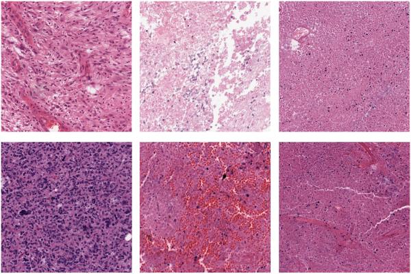
GBM Examples. First column: Tumor; Second column: Transition to necrosis; Third column: Necrosis.

Table 1.

Performance of different methods on the GBM dataset

	Method	DictionarySize=256	DictionarySize=512	DictionarySize=1024
160 training	PSDSPM	91.02 ± 1.89	91.41 ± 0.95	91.20 ± 1.29
	PSD [1]	86.07 ± 1.42	86.32 ± 1.14	86.15 ± 1.33
	ScSPM [12]	79.58 ± 0.61	81.29 ± 0.86	82.36 ± 1.10
	KSPM [2]	85.00 ± 0.79	86.47 ± 0.55	86.81 ± 0.45
80 training	PSDSPM	88.63 ± 0.91	88.91 ± 1.18	88.64 ± 1.08
	PSD [1]	81.73 ± 0.98	82.08 ± 1.23	81.55 ± 1.17
	ScSPM [12]	77.65 ± 1.43	78.31 ± 1.13	81.00 ± 0.98
	KSPM [2]	83.81 ± 1.22	84.32 ± 0.67	84.49 ± 0.34
40 training	PSDSPM	84.06 ± 1.16	83.72 ± 1.46	83.40 ± 1.14
	PSD [1]	78.28 ± 1.74	78.15 ± 1.43	77.97 ± 1.65
	ScSPM [12]	73.60 ± 1.68	75.58 ± 1.29	76.24 ± 3.05
	KSPM [2]	80.54 ± 1.21	80.56 ± 1.24	80.46 ± 0.56

4.2 KIRC Dataset

The KIRC dataset contains 3 classes: Tumor, Normal, and Stromal, which were curated from WSI scanned with a 40× objective. Examples can be found in Figure 4. The number of images per category are 568, 796 and 784, respectively. Most images are 1000 × 1000 pixels. In this experiment, we trained on 70, 140 and 280 images per category and tested on the rest, with three different dictionary sizes: 256, 512 and 1024. Detailed comparisons are shown in Table 2.

Fig. 4.

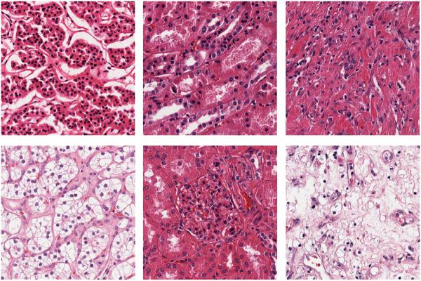
KIRC Examples. First column: Tumor; Second column: Normal; Third column: Stromal.

Table 2.

Performance of different methods on the KIRC dataset

	Method	DictionarySize=256	DictionarySize=512	DictionarySize=1024
280 training	PSDSPM	97.19 ± 0.49	97.27 ± 0.44	97.08 ± 0.45
	PSD [1]	90.72 ± 1.32	90.18 ± 0.88	90.43 ± 0.80
	ScSPM [12]	94.52 ± 0.44	96.37 ± 0.45	96.81 ± 0.50
	KSPM [2]	93.55 ± 0.31	93.76 ± 0.27	93.90 ± 0.19
140 training	PSDSPM	96.80 ± 0.75	96.52 ± 0.76	96.55 ± 0.84
	PSD [1]	88.75 ± 0.37	88.93 ± 0.45	87.98 ± 0.86
	ScSPM [12]	93.46 ± 0.55	95.68 ± 0.36	96.76 ± 0.63
	KSPM [2]	92.50 ± 1.12	93.06 ± 0.82	93.26 ± 0.68
70 training	PSDSPM	95.12 ± 0.54	95.13 ± 0.51	95.09 ± 0.40
	PSD [1]	87.56 ± 0.78	87.93 ± 0.67	87.13 ± 0.97
	ScSPM [12]	91.93 ± 1.00	93.67 ± 0.72	94.86 ± 0.86
	KSPM [2]	90.78 ± 0.98	91.34 ± 1.13	91.59 ± 0.97

The experiments, conducted on two distinct datasets of vastly different tumor types, indicate that,

1. SPM improves the performance for tissue classification. As shown in Tables 1 and 2, PSDSPM consistently outperforms PSD, which demonstrates the effectiveness of SPM for tissue classification. We suggest that the improvement of performance is due to the local histogramming involved in SPM, which provides some sort of tissue morphometric context at various locations and scales. In practice, the context information is widely adopted by well trained pathologists for diagnosis.

2. Features from unsupervised feature learning are more tolerant to batch effect than human engineered features for tissue classification. As shown in Tables 1 and 2, PSDSPM consistently outperforms KSPM. Since the only difference between these two approaches is that PSDSPM utilize features from unsupervised feature learning, while KSPM is based on human engineered features (SIFT), we suggest that, given the large amounts of technical and biological variations in the TCGA datasets, features from unsupervised feature learning are more tolerant to batch effect than human engineered features for tissue classification.

As a result, the combination of unsupervised feature learning and SPM leads to an approach with following merits,

1. Extensibility to different tumor types. Tables 1 and 2 indicate that, our method consistently outperforms [12,2,1]. However, due to the poor generalization ability of human engineered feature (SIFT), KSPM and ScSPM appear to be tumor-type dependent. Since GBM and KIRC are two vastly different tumor types with significantly different signatures, we suggest that the consistency in performance assures extensibility to different tumor types.

2. Robustness in the presence of large amounts of technical and biological variations. For the GBM dataset, shown in Table 1, the performance of PSDSPM, with 80 training samples per category, is better than the performance of [12,2,1] with 160 training samples per category. For the KIRC dataset, shown in Table 2, the performance of PSDSPM, with 140 training samples per category, is either better than or comparable to the performance of [2,1,12] with 280 training samples per category. These results clearly indicate the robustness of our approach, which improves the scalability with varying training sample size, and the reliability of further analysis on large cohort of WSI.

In our approach, the choice of PSD for unsupervised feature learning, over others (e.g., Reconstruction Independent Subspace Analysis (RISA) [9]), is due to its effectiveness and efficiency in a feed-forward fashion, which is demonstrated by an experimental comparison with RISA, based on the dataset and protocols in [9], as shown in Table 3.

Table 3.

Comparison of performance among PSDSPM, PSD and RISA

PSDSPM	PSD	RISA
96.50	95.05	91.10

5 Conclusion and Future Work

In this paper, we proposed a SPM approach based on sparse tissue morphometric features from unsupervised feature learning, for tissue image classification. Due to the robustness of unsupervised feature learning and the effectiveness of the SPM framework, our method outperforms traditional ones which were typically based on human engineered features. The most encouraging results of this paper are that, our methods are highly i) extensible to different tumor types; ii) robust in the presence of large amounts of technical and biological variations; and iii) scalable with varying training sample sizes. Future work will be focused on utilizing supervised dictionary learning [14] for possible improvement, and further validating our methods on other tissue types.

6 Disclaimer

This document was prepared as an account of work sponsored by the United States Government. While this document is believed to contain correct information, neither the United States Government nor any agency thereof, nor the Regents of the University of California, nor any of their employees, makes any warranty, express or implied, or assumes any legal responsibility for the accuracy, completeness, or usefulness of any information, apparatus, product, or process disclosed, or represents that its use would not infringe privately owned rights. Reference herein to any specific commercial product, process, or service by its trade name, trademark, manufacturer, or otherwise, does not necessarily constitute or imply its endorsement, recommendation, or favoring by the United States Government or any agency thereof, or the Regents of the University of California. The views and opinions of authors expressed herein do not necessarily state or reflect those of the United States Government or any agency thereof or the Regents of the University of California.

References

- 1.Kavukcuoglu K, Ranzato M, LeCun Y. Technical Report CBLL-TR-2008-12-01. Computational and Biological Learning Lab, Courant Institute, NYU; 2008. Fast inference in sparse coding algorithms with applications to object recognition. [Google Scholar]
- 2.Lazebnik S, Schmid C, Ponce J. Beyond bags of features: Spatial pyramid matching for recognizing natural scene categories; Proceedings of the Conference on Computer Vision and Pattern Recognition; 2006.pp. 2169–2178. [Google Scholar]
- 3.Gurcan M, Boucheron L, Can A, Madabhushi A, Rajpoot N, Bulent Y. Histopathological image analysis: a review. IEEE Reviews in Biomedical Engineering. 2009;2:147–171. doi: 10.1109/RBME.2009.2034865. [DOI] [PMC free article] [PubMed] [Google Scholar]
- 4.Ghaznavi F, Evans A, Madabhushi A, Feldman M. Digital imaging in pathology: whole-slide imaging and beyond. Annu. Rev. Pathology. 2012;8:331–359. doi: 10.1146/annurev-pathol-011811-120902. [DOI] [PubMed] [Google Scholar]
- 5.Ali S, Madabhushi A. An integrated region-, boundry-, and shape-based active contour for multiple object overlap resolution in histological imagery. IEEE Transactions on Medical Imaging. 2012;31(7):1448–1460. doi: 10.1109/TMI.2012.2190089. [DOI] [PubMed] [Google Scholar]
- 6.Chang H, Han J, Borowsky A, Loss L, Gray JW, Spellman PT, Parvin B. Invariant delineation of nuclear architecture in glioblastoma multiforme for clinical and molecular association. IEEE Transactions on Medical Imaging. 2013;32(4):670–682. doi: 10.1109/TMI.2012.2231420. [DOI] [PMC free article] [PubMed] [Google Scholar]
- 7.Kothari S, Phan J, Osunkoya A, Wang M. Biological interpretation of morphological patterns in histopathological whole slide images; ACM Conference on Bioinformatics, Computational Biology and Biomedicine; 2012; [DOI] [PMC free article] [PubMed] [Google Scholar]
- 8.Nayak N, Chang H, Borowsky A, Spellman PT, Parvin B. Classification of tumor histopathology via sparse feature learning. International Symposium on Biomedical Imaging; 2013; [DOI] [PMC free article] [PubMed] [Google Scholar]
- 9.Le Q, Han J, Gray J, Spellman P, Borowsky A, Parvin B. Learning invariant features from tumor signature. International Symposium on Biomedical Imaging; 2012.pp. 302–305. [Google Scholar]
- 10.Everingham M, Van Gool L, Williams CKI, Winn J, Zisserman A. The PASCAL Visual Object Classes Challenge (VOC 2012) Results. 2012 http://www.pascal-network.org/challenges/VOC/voc2012/workshop/index.html.
- 11.Vedaldi A, Zisserman A. Efficient additive kernels via explicit feature maps. IEEE Transactions on Pattern Analysis and Machine Intelligence. 2012;34(3):480–492. doi: 10.1109/TPAMI.2011.153. [DOI] [PubMed] [Google Scholar]
- 12.Yang J, Yu K, Gong Y, Huang T. Linear spatial pyramid matching using sparse coding for image classification; Proceedings of the Conference on Computer Vision and Pattern Recognition; 2009.pp. 1794–1801. [Google Scholar]
- 13.Fan RE, Chang KW, Hsieh CJ, Wang XR, Lin CJ. LIBLINEAR: A library for large linear classification. Journal of Machine Learning Research. 2008;9:1871–1874. [Google Scholar]
- 14.Mairal J, Bach F, Ponce J, Sapiro G, Zisserman A. NIPS. 2008. Supervised dictionary learning. [Google Scholar]