Principal Component Analysis in Construction of 3D Human Knee Joint Models Using a Statistical Shape Model Method

Abstract

The statistical shape model (SSM) method that uses 2D images of the knee joint to predict the 3D joint surface model has been reported in literature. In this study, we constructed a SSM database using 152 human CT knee joint models, including the femur, tibia and patella and analyzed the characteristics of each principal component of the SSM. The surface models of two in vivo knees were predicted using the SSM and their 2D bi-plane fluoroscopic images. The predicted models were compared to their CT joint models. The differences between the predicted 3D knee joint surfaces and the CT image-based surfaces were 0.30 ± 0.81 mm, 0.34 ± 0.79 mm and 0.36 ± 0.59 mm for the femur, tibia and patella, respectively (average ± standard deviation). The computational time for each bone of the knee joint was within 30 seconds using a personal computer. The analysis of this study indicated that the SSM method could be a useful tool to construct 3D surface models of the knee with sub-millimeter accuracy in real time. Thus it may have a broad application in computer assisted knee surgeries that require 3D surface models of the knee.

1. INTRODUCTION

Subject-specific three-dimensional (3D) knee models have been widely used in orthopaedics and biomechanics research, such as pre-operative surgical planning, surgical navigation, and development of arthroplasty and surgical techniques (Huang et al., 2011; Matziolis et al., 2007). Currently, 3D bone models can be obtained from computed tomography (CT) scans with sub-millimeter accuracy (Liang et al., 2010). The images could be automatically processed with certain manual operation (Kang et al., 2003). However, the radiation exposure with CT causes concerns of potential risks that limit its application. An alternative modeling procedure is through magnetic resonance imaging (MRI), which requires prolonged scanning time and extensive manual operation (DeFrate et al., 2004) or sophisticate automatic image segmentation (Fripp et al., 2010). An accurate and efficient method for the construction of 3D knee joint models has been pursued for decades (Baka et al., 2011; Cootes et al., 1995; Dong and Zheng, 2009; Zheng et al., 2006; Zheng et al., 2010).

Recently, statistical shape model (SSM) method has been developed as a promising tool for the reconstruction of subject-specific 3D joint models. In this method, an SSM database of 3D joint models is constructed to define the common characteristics of the knee joint surface geometry through the Principal Component Analysis (PCA) (Seber, 1984). The 3D surface of a new target joint can be computed by matching the geometric characteristics extracted from one or multiple plain radiographic images of the joint to the principal components of the SSM (Heimann and Meinzer, 2009). There are few studies that have reconstructed the patient-specific 3D models of the proximal and/or distal femur (Barratt et al., 2008; Laporte et al., 2003; Tang and Ellis, 2005; Zhu and Li, 2011) and patella (Chen et al., 2010) with an accuracy around 1 mm. However, the accuracy and efficiency of applying the SSM for reconstruction of the whole knee joint, including distal femur, tibia and patella bones have not been evaluated.

The overall objective of this study is to examine the feasibility, accuracy and efficiency of predicting 3D human knee joint models using the SSM and 2D dual fluoroscopic images. First, a 3D SSM knee CT database was built using 3D knee joint models including distal femur, proximal tibia and patella. By means of the SSM and the dual-fluoroscopic images of a target knee, we reconstructed the knee model and compared the predicted model with the corresponding CT-based model. Furthermore, we investigate the effect of the number of principal components on the accuracy and computational time in the SSM.

2. MATERIALS & METHODS

2.1 Statistical Shape Model of the Knee

The SSM method uses a population of the 3D shape models of the target joint to construct a training basis (S_i), which is also called point distribution model (PDM) in literature (Zheng et al., 2006). For the construction of the basis, each bony surface (distal femur, proximal tibia and patella) was automatically aligned by the method of the iterative closest points (Besl and McKay, 1992). Aligned surface models were used to build corresponding point sets of each of the distal femur, proximal tibia and patella with previous published template method (Zhu and Li, 2011). Three templates with 4000 evenly distributed standard nodal points (x_i, y_i, z_i) were created according to the geometric features for each bone. For the femur, two spherical coordinates and a cylindrical coordinate were adopted for the condyles and the shaft. For the tibia, one spherical coordinates and a cylindrical system were adopted for the tibia plateau and shaft. For the patellar, a spherical coordinate was used. The sample set of each bone was used to build a co-variance matrix (Cov) for each PDM from the sample set (S_i).

$$\{\mathit{Cov}=\frac{1}{p-1}\sum _{i=1}^p(S_i-\overline{S}){(S_i-\overline{S})}^T,\mathit{with}{S}_i={(x_1,y_1,z_1\cdots x_n,y_n,z_n)}^T,\overline{S}=\frac{1}{p}\sum _{i=1}^p{S}_i,i=1:p,$$ (1)

where p is the number of knees in the sample set and n is the nodal number of each model.

A principal component analysis (PCA) method (Wold et al., 1987) is used to analyze the covariance matrix of the PDM. The PCA for the knee models captures geometric features of the model population using the eigenvalues and eigenvectors of the co-variance matrix (Zhu and Li, 2011).

$$\{\begin{array}{l}\mathit{eigenvalue}=({\lambda }_1,{\lambda }_2,\cdots {\lambda }_s),{\lambda }_1\ge {\lambda }_2\cdots \ge {\lambda }_s\ge 0\hfill \\ \mathit{eigenvector}=(P_1,P_2,\cdots P_s)\hfill \end{array},$$ (2)

Where the dimension of P_j is 1×(3n). The first principal component with the largest eigenvalue stands for the greatest variation depending on the direction and location among all models. The second principal component with the second largest eigenvalue stands for the second greatest variation and so on.

The SSM is then represented by the average joint model (S̄), the eigenvalues and eigenvectors. Any specific joint shape, S′, could then be predicted using the SSM method in the following formula (Cootes et al., 1995),

$$\{\begin{array}{l}{S}^{\prime }=M\overline{S}+M\sum _{j=1}^{s}f({\lambda }_j)P_j\hfill \\ f({\lambda }_j)=a_j\sqrt{{\lambda }_j}\hfill \\ M=\frac{1}{p}\sum _{i=1}^p{M}_i\hfill \end{array},$$ (3)

Where p is the number of the principal components used in the prediction, a_j is the s weight factors used to generate the new shape model, and M_i is the transformation matrix that transforms the i-th knee model in the SSM from its local coordinate system to the global coordinate system.

To predict a shape model of an actual joint, the weight factors, a_j, needs to be determined using the information of the target joint (Cootes et al., 1995), usually obtained from one or multiple radiographic images of the target joint. In this paper, we used bi-plane fluoroscopic images from a dual orthogonal fluoroscopic system (Bingham and Li, 2006).

2.2 Construction of the SSM

Subject Demographics

The population of the 3D shape models of the knee that was used to construct the SSM was obtained from 34 males and 46 females with no history of knee pain, knee pathologies, and anatomical abnormality. The age ranged from 36 to 62 years (51.1±6.6) for the male subjects and 22 to 54 years (43.5±6.2) for the female subjects. Both knees of each subject were included except for 8 knees due to their osteophytes and bone irregularity. A total of 152 knees were included. Each knee was CT scanned (LightSpeed Plus, GE Medical Systems, Waukesha, Wisconsin) from 25 cm above and below the joint line to acquire axial CT slices of 1.25 mm in thickness and 0.7×0.7 mm in-plane pixel resolution. The knee bones were segmented using a region-growing method (Adams and Bischof, 1994). The segmented contours were then reviewed and manually corrected by an orthopaedic surgeon. The contours were imported to a solid modeling program (Rhinoceros, Robert McNeel & Associates, Seattle, WA) for construction of a 3D knee joint model (Li et al., 2008) (Fig. 1).

Figure 1.

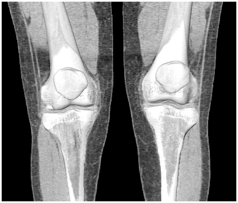
Bilateral knee joint models of a subject, including the distal femur, proximal tibia and patella, reconstructed from CT images.

2D/3D Reconstruction

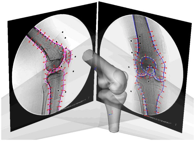
The new SSM surface of any actual knee joint, S′, can be deformed based on the average model (S̄) and the principle components by determination of the weight factors, a_j in Eq. 3. We adopted the method of using 2D fluoroscopic images of the joint to determine the shape model (Lamecker et al., 2004; Tang and Ellis, 2005; Zheng and Schumann, 2009; Zhu and Li, 2011). In this paper, a joint was imaged using a synchronized dual orthogonal fluoroscopic system (Fig. 2) (Bingham and Li, 2006). The dual-fluoroscopic images were imported into the solid software (Rhinoceros) to construct a virtual fluoroscopic system (Bingham and Li, 2006). The SSM was then introduced in the virtual fluoroscopic system and projected on the two fluoroscopic images of the target joint. Through an optimization procedure, the weight factors, a_j, was adjusted using the outline information of the joint from its 2D projected images, so that the differences between the outlines of the SSM shape model (L₁) and the outlines of the actual joint (L₂) were minimized (objective function F):

$$F=\underset{\{a_j\}}{min}\left(\sum _{k=1}^n\left|L_1^k-L_2^k\right|\right),$$ (4)

where n is the number of 2D images and k represents the k -th 2D image. At each step of the optimization, the set of weights (a_j) will be used to obtain a new SSM surface S′ through Eq. 3. Therefore, the converged 3D SSM surface S′ can be used to represent the actual knee joint model.

Figure 2.

Environment setup for the SSM in a virtual dual fluoroscope imaging system. Average models, including the femur, tibia and patella were imported and positioned to match the silhouettes on the dual fluoroscopic images. Corresponding SSM would deform to fit the outlines of dual fluoroscopic images. Solid line: actual joint outline. Dashed white line: projection of the average models.

2.3 Principal Component Analysis of the SSM

A series of parametric analyses were conducted to evaluate the feasibility of the SSM models in prediction of the knee models. In application of the SSM represented by Eq. 3, each principal component and eigenvalue represented a different geometric feature of the 3D bony surface (Lorenz and Krahnstöver, 2000). The contribution of major to minor principal components to the corresponding location of geometric deformation on the average models of the femur, tibia and patella were analyzed. In addition, we examined the effects of the number of principle components on two living knees by determining the differences between the predicted joint surfaces and the CT models of the knee. The differences of the projected contour and the segmented fluoroscopic features (objective function in Eq. 4) were also calculated with respect to the number of principal components of the SSM. All optimizations were performed using a PC (Intel(R) Core(TM) i7-2600 processor: 3.40 GHz, 8 GB RAM) on MATLAB (MathWork, Natick, MA) platform.

2.4 Accuracy of the SSM Method

Two living health knees were included for the validity of SSM. Each knee was imaged using a dual fluoroscopic system to obtain two images of the knee from orthogonal directions (Zhu and Li, 2011). The predicted SSM surfaces through the optimization procedure using different numbers of principal components were also compared to the corresponding native 3D knee joint models constructed using their CT images, which are considered as the ground truth in this paper. In order to calculate the differences between the predicted model and the CT model (termed as error in this paper), the distance between each point of the SSM prediction and the CT model surface was calculated. The points outside of CT model were defined as positive error and inside were negative. The average (Avg) errors, standard deviation (Std), the maximum (Max) errors, and the average of the absolute values of the errors (ABS Avg) were reported.

3. RESULTS

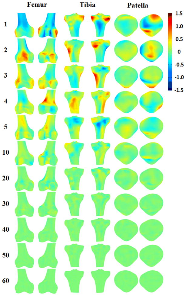
The magnitudes of the eigenvalues decayed exponentially for each bone of the knee (Fig. 3). 3D surfaces rendering of the effect of the principal component on the average femur, tibia and patella were shown in different views (Fig. 4). The first eigenvalues of the femur, tibia and patella database were about 950, 800 and 500 (25.7%, 20.1% and 18.59% of total variation), respectively, while the 10th eigenvalues decreased to around 100. The 30th eigenvalues dropped to close to 0. With the magnitude of the eigenvalue decayed, the effects of major to minor principal components on the average model gradually decreased (Fig. 4).

Figure 3.

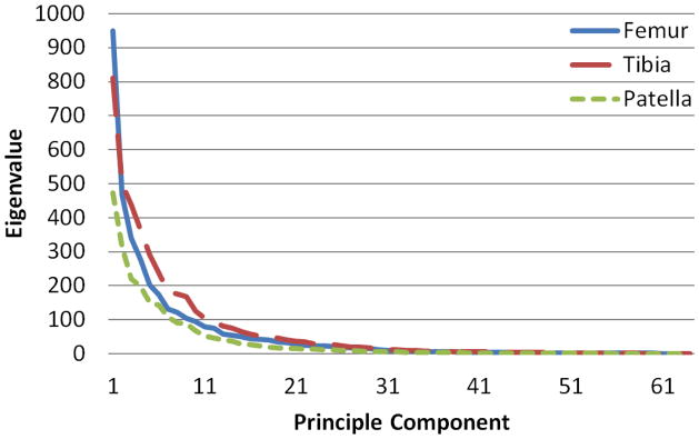
Eigenvalues against principle component numbers of covariance matrices of the point distribution models of the femur, tibia and patella. The magnitudes of the eigenvalues tend to be flat from 30th component, meaning the successive components are accounting for smaller amounts of the total variance.

Figure 4.

3D surface rendering of SSMs of the femur, tibia and patella with color representing of the difference of each principal component on the average model. Positive or negative values indicate that predicted nodes were inside or outside of the average model. The first few principal components account for most of the total variance in the SSM.

For the femur, the effects of the first principal component would dilate the lateral and medial epicondyles, erode the intercondylar fossa and adjust the radius of the shaft. The second principal component would dilate the patella surface, the posterior part of the lateral condyle. The third principle component would dilate the distal part of the medial condyle and the lateral and medial epicondyle. For the tibia, the first principal component would dilate medial and lateral condyles and adjust the radius of the shaft. The second principal component would dilate the tibial tuberosity and medial posterior condyle. The third principal component would dilate medial and lateral side of the tibial shaft. For the patella, the first principal component would dilate the medial superior and lateral inferior articular surfaces. The second principal component would dilate the ridge. The third principal component would dilate the apex. The effects of principle component after the third were getting smaller (Fig. 4).

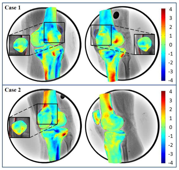
The overall i differences between the 3D SSM surface and CT model surface were 0.30 ± 0.81 mm, 0.34 ± 0.79 mm 0.36 ± 0.59 mm for femur, tibia and patella, respectively using the full set of principal components (Table 1). Errors of points on SSM in the interior of the CT models were considered negative. The mean values of the max outside error were 3.48 mm, 3.23 mm, and 2.15 mm for femur, tibia and patella, respectively. The corresponding max inside error was −3.34 mm, −3.67 mm, and −2.14 mm. The locations of minimum errors were along the edge in the projection directions of the corresponding 2D orthogonal dual fluoroscope images (Fig. 5). The locations of the maximum errors were on the concave surfaces or away from the tangent area of the dual fluoroscopic projection (Fig. 5), where information on the bony outline was limited.

Table 1.

The average (Avg), standard deviation (Std), maximum (Max), minimum (Min) and average of absolute distance (ABS Avg) of the differences between predicted model and CT reconstructed models of distal femur, proximal tibia and patella for four in vivo cases (unit: mm). Positive or negative values represent that predicted nodes were inside or outside of the CT models.

Case	Femur					Tibia					Patella
	Avg	Std	Max	Min	ABS Avg	Avg	Std	Max	Min	ABS Avg	Avg	Std	Max	Min	ABS Avg
Left-case1	0.30	0.97	3.90	−2.82	0.80	0.48	0.53	2.11	−3.16	0.17	0.49	0.60	2.70	−2.09	0.06
Left-case2	0.46	0.76	3.83	−3.03	0.66	0.51	0.56	2.27	−2.56	0.11	0.57	0.59	2.39	−2.76	0.03
Right-case1	0.33	0.72	3.31	−3.64	0.60	0.16	1.09	4.46	−4.34	0.80	0.20	0.51	1.89	−1.69	0.39
Right-case2	0.11	0.80	2.89	−3.85	0.62	0.22	0.98	4.09	−4.62	0.73	0.19	0.67	1.61	−2.00	0.56
Mean	0.30	0.81	3.48	−3.34	0.67	0.34	0.79	3.23	−3.67	0.45	0.36	0.59	2.15	−2.14	0.26
SD	0.14	0.11	0.47	0.49	0.09	0.18	0.29	1.21	0.97	0.36	0.20	0.07	0.49	0.45	0.26

Figure 5.

3D surface rendering of SSMs of the femur, tibia and patella with color representing of the difference from CT reconstruction models. Positive or negative values indicate that predicted nodes were inside or outside of the CT models. The surface of SSMs close to the digitized contours on fluoroscopic images showed smaller differences.

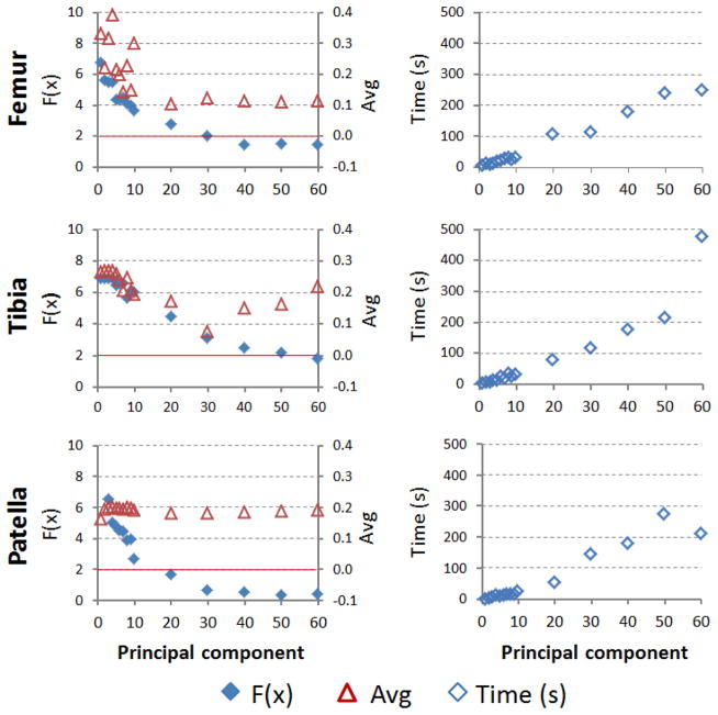
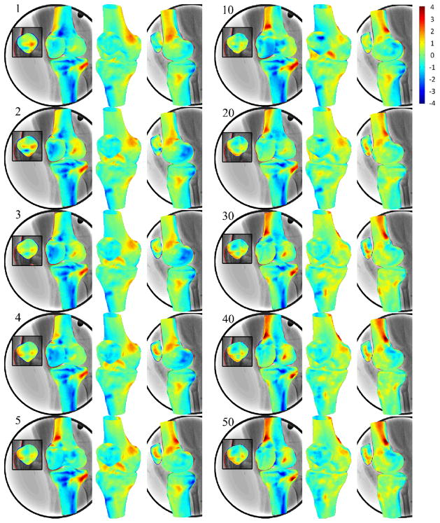
Less number of principal components for SSM prediction resulted in shorter computational time (Fig. 6 & Table 2). Using SSM with 7 principal components, the computational time for prediction of each of the femur, tibia and patella was less than 30s. The accuracy of the predicted surface models was not dramatically affected by the number of principal components used (Table 2). The average differences between the predicted model and CT model were slightly decreasing from 0.33 mm using 1 component to 0.11 mm using 40 components. However, the standard deviation, maximum, minimum and average absolute value of the model differences do not change with different numbers of principal components used for surface prediction (Table 2).

Figure 6.

The effects of using different number of principle components in SSM on 2D projection differences on the fluoroscopic images, 3D average error of the predicted surface and computational time.

Table 2.

The average (Avg), standard deviation (Std), maximum (Max), minimum (Min) and average of absolute distance (ABS Avg) of the differences between predicted SSM and CT reconstructed models of distal femur, proximal tibia and patella with different nodal numbers in the SSM (unit: mm). Positive or negative values represent that predicted nodes were inside or outside of the CT models. Computational time was also provided (unit: second).

Numbers of principal component	Femur							Tibia							Patella
	Time (s)	F(x)	Avg	Std	Max	Min	ABS Avg	Time (s)	F(x)	Avg	Std	Max	Min	ABS Avg	Time (s)	F(x)	Avg	Std	Max	Min	ABS Avg
1	5.0	6.7	0.33	0.79	3.74	−2.32	0.68	3.1	6.85	0.26	0.97	3.07	−3.07	0.75	1.3	17.31	0.16	0.78	1.79	−2.47	0.67
2	10.2	5.6	0.22	0.83	3.15	−2.44	0.68	4.8	6.86	0.27	0.96	3.07	−3.02	0.75	3.6	11.13	0.19	0.84	3.01	−2.20	0.73
3	9.1	5.5	0.32	0.84	3.17	−2.28	0.71	5.5	6.86	0.27	0.96	3.07	−3.02	0.75	6.7	6.56	0.20	0.69	1.86	−1.95	0.58
4	12.7	5.5	0.39	0.86	3.06	−2.38	0.75	12.9	6.85	0.27	0.97	3.07	−3.06	0.76	11.3	5.02	0.20	0.76	2.00	−2.43	0.63
5	17.7	4.4	0.21	0.90	2.46	−3.51	0.73	12.0	6.40	0.26	1.05	3.27	−3.72	0.81	9.2	4.74	0.20	0.73	1.86	−2.29	0.62
6	21.6	4.3	0.20	0.90	2.61	−3.62	0.72	23.7	6.56	0.24	1.04	3.21	−3.70	0.80	12.6	4.50	0.20	0.70	1.93	−2.11	0.60
7	27.4	4.4	0.14	0.98	2.92	−4.34	0.76	16.5	6.57	0.21	1.03	2.98	−3.60	0.78	16.5	4.42	0.20	0.69	1.89	−2.13	0.58
8	29.3	4.1	0.23	0.92	2.37	−3.60	0.74	34.2	5.61	0.25	1.25	3.80	−4.53	0.98	17.0	3.90	0.20	0.69	2.89	−1.47	0.58
9	24.6	3.9	0.15	0.93	2.66	−4.21	0.73	22.9	6.06	0.20	1.08	3.36	−3.65	0.83	15.0	3.92	0.20	0.68	2.60	−1.55	0.58
10	29.6	3.6	0.30	0.96	2.62	−3.68	0.78	29.0	6.01	0.19	1.08	3.35	−3.71	0.83	24.2	2.70	0.19	0.81	3.91	−1.46	0.62
20	106.6	2.7	0.10	0.81	2.31	−2.80	0.65	79.2	4.42	0.17	0.95	3.57	−3.26	0.72	54.5	1.64	0.18	0.76	2.82	−2.34	0.60
30	111.7	2.0	0.12	0.84	3.51	−3.89	0.64	114.6	3.05	0.08	0.94	3.57	−3.97	0.69	146.5	0.64	0.18	0.74	1.82	−2.55	0.62
40	177.3	1.4	0.11	0.89	3.63	−4.51	0.68	175.3	2.45	0.15	0.90	3.63	−4.27	0.65	181.0	0.52	0.19	0.72	1.63	−2.20	0.60
50	239.0	1.4	0.11	0.89	3.46	−4.52	0.68	214.6	2.16	0.16	0.91	3.69	−4.27	0.67	275.8	0.32	0.19	0.77	1.85	−2.11	0.64
60	249.4	1.4	0.11	0.80	2.89	−3.85	0.62	477.0	1.74	0.22	0.98	4.09	−4.62	0.73	210.5	0.37	0.19	0.67	1.61	−2.00	0.56

4. DISCUSSION

The SSM method has the potential to predict patient-specific 3D models instead of using 3D CT or MR images. In this study, a SSM of the knee joint was constructed with 152 knee joint models from 80 health adults. New 3D knee joint surface models including the femur, tibia and patella can be predicted using the SSM with two 2D orthogonal fluoroscopy images of the target knee (Zhu and Li, 2011). Validation of the accuracy and precision was conducted by comparing the differences between the predicted model and the CT model. The overall accuracies of the predicted model surfaces were within 0.30 ± 0.81 mm, 0.34 ± 0.79 mm and 0.36 ± 0.59 mm for the femur, tibia and patella, respectively. The computational time can be controlled within 30 seconds by using only major principal components for each bone model without losing accuracy and precision.

The SSM method has been validated and applied to different human joints, such as the lumbar vertebra, pelvis, and proximal and distal femur (Buchaillard et al., 2007; Fleute et al., 1999; Laporte et al., 2003; Luthi et al., 2009; Rajamani et al., 2007; Sadowsky et al., 2007; Styner et al., 2003; Tang and Ellis, 2005; Zheng et al., 2011; Zhu and Li, 2011). Fleute et al. (Fleute et al., 1999) used 11 proximal and distal femur models to construct a SSM. Intra-operative digitized points were collected on the joint surface to predict the model. Results showed average accuracies of 1.6~2.2 mm. Laporte et al. (Laporte et al., 2003) utilized a SSM constructed from 8 CT knee models and two orthogonal images of the knee to reconstruct the target femur shape with an accuracy of 1.0 mm and a RMS of 1.3 mm. Tang and Ellis (Tang and Ellis, 2005) used 20 femoral CT models to construct a SSM. Results of simulated projections and fluoroscopic images of cadaver knees show that the femoral shape models can be predicted with an accuracy of about 2 mm.

More recently, Zhu and Li reported an improved accuracy for prediction of human distal femur surfaces (0.16±1.16 mm) with a dual fluoroscopic setup and a SSM constructed using 40 MRI models (Zhu and Li, 2011). They showed that at least 2 views of the knee are needed for the reconstruction of the femur model. The average error dropped from 0.27 using one image to 0.03 mm using more than two images. We used a similar dual fluoroscopy imaging system to capture two orthogonal images in this study and the distal femur bone can be predicted with a comparable accuracy of 0.30±0.81 mm. There is limited report on the validation and application of the SSM method used for the tibia and patella bones. We obtained similar or slightly better accuracy and precision for the tibia and patella bones (0.34±0.79 mm and 0.36±0.59 mm, respectively) as for the femur. This is possibly due to less irregularity and concaved surface on the latter two compare to the femur. With less irregularity, the 2D bony outlines can better capture the 3D shape characters and thus reduce the corresponding errors due to local irregular geometries.

Parametric analysis of the SSM showed that the first few principle components represent the major variances of the surface models in the population (Fig. 3&4). An efficiency test of the SSM was achieved by reducing the number of principal components used in the SSM prediction (Table 2). Results showed that the 2D projection differences became smaller while the number of principal component increased (Fig. 6). However, the average difference of the 3D surface model with respect to the CT model does not have the same trend. The average difference of the distal femur can be improved while increasing the number of principle components from 1 to 20 (Fig. 6), but not beyond. For the tibia, the averaged difference reduced to 30 principle components. For the patella, no obvious trend can be observed. This might be attributed to the dual fluoroscopic images can only capture bone projections which contains 2D information and cannot capture the features of higher order principal components. Therefore, reduction of the dimensionality of the SSM dataset by deleting the high order principal components did not significantly decrease the accuracy of the predicted models but could dramatically reduce the computational time from 4 min to 30 sec for the femur (Table 2). Overall, the calculation time in this study was improved compared to other studies. Baka et al. used biplane fluoroscopic images to construct the distal femur model and the computational time was about five minutes (Baka et al., 2011) and the calculation time from Zhu et al. was about 71 seconds (Zhu and Li, 2011). Other authors (Fleute et al., 1999; Laporte et al., 2003; Tang and Ellis, 2005) also investigated the effect of only using first few principal components on the overall accuracy of the predicted model. For example, the first few principal components accounted for most of the variance of the knee model and the residual fitting errors dropped from 2.1 to 1.7 mm with 2 and 6 modes, in Fleute et al.’s study (Fleute et al., 1999). Using a few major principal components could be sufficient to capture most of the variability in the original dataset for prediction of a knee joint model.

In our study, the weighting factors of each component were adjusted to get a best fit of the model projections to the contours on the dual fluoroscopic images (Eq. 2). Since the contours on the fluoroscopic images were fit using the projection outline information of the joint model, the part of the tangent surfaces could fit the projection well (Table 2). The other parts of the surface which were not parallel to the projection direction were estimated based on the SSM (Fig. 7). Features of the bone which were not captured by fluoroscopic images were estimated using weighted combinations of the principal components. Those parts of surfaces hidden inside or behind, located where the dual fluoroscope cannot capture, had relative higher discrepancy with CT models (Fig. 5). Different projection directions of dual fluoroscopes relative to the knee would affect the location of the tangent surfaces which might change the error distribution on the predicted model. Based on our current results, the average difference showed good agreement of the estimated models and the CT models (Table 1), which implied that the characteristics of the target model were in agreement with the characteristics of the population in SSM.

Figure 7.

3D surface rendering of SSMs of the femur, tibia and patella with color representing of the difference from CT reconstruction models. Positive or negative values indicate that predicted nodes were inside or outside of the CT models. Numbers on the upper left indicated the number of principal components used in SSM for prediction. While the number of the principal components increasing in SSM, the 2D projection of the SSM getting closer to the contours on fluoroscopic images.

The accuracy of the predicted models can be affected by different knee joint models training basis, due to the possible different features of the bones used in the database. Yue et al. indicated that there are different features of the knee joint between male and female, and between a Caucasian and a Chinese population (Yue et al., 2011). Further investigations on the effects of different populations and sex might be needed for construction of different SSMs. Surface models of the knee have been used in many aspects, e.g. surgical planning, computer-aided navigation and morphological analysis. Results of the current study indicated that the proposed method could be used to construct 3D surface models of the knee in real time, suggesting that the integration of SSM and dual fluoroscopic imaging might be a promising tool for further applications.

4. CONCLUSION

A SSM for construction of 3D knee joint models has been developed in this study. The overall (outside and inside) accuracies of the 3D SSM model surfaces were 0.30 ± 0.81 mm, 0.34 ± 0.79 mm and 0.36 ± 0.59 mm for the distal femur, proximal tibia and patella, respectively. The computational time for the whole knee joint could be controlled within one minute on a common personal computer. The analysis of this study indicated that the SSM method could be used to construct 3D surface models of the knee in real time and might be a useful tool for computer assisted knee surgeries without using CT or MR images.

References

- Adams R, Bischof L. Seeded Region Growing. Pattern Analysis and Machine Intelligence, IEEE Transactions on. 1994;16(6):641–647. Available from: http://ieeexplore.ieee.org/xpls/abs_all.jsp?arnumber=295913. [Google Scholar]
- Baka N, Kaptein BL, de Bruijne M, van Walsum T, Giphart JE, Niessen WJ, Lelieveldt BP. 2d–3d Shape Reconstruction of the Distal Femur from Stereo X-Ray Imaging Using Statistical Shape Models. Med Image Anal. 2011;15(6):840–850. doi: 10.1016/j.media.2011.04.001. Available from: http://www.ncbi.nlm.nih.gov/pubmed/21600836. [DOI] [PubMed] [Google Scholar]
- Barratt DC, Chan CS, Edwards PJ, Penney GP, Slomczykowski M, Carter TJ, Hawkes DJ. Instantiation and Registration of Statistical Shape Models of the Femur and Pelvis Using 3d Ultrasound Imaging. Med Image Anal. 2008;12(3):358–374. doi: 10.1016/j.media.2007.12.006. Available from: http://www.ncbi.nlm.nih.gov/pubmed/18313973. [DOI] [PubMed] [Google Scholar]
- Besl PJ, McKay ND. A Method for Registration of 3-D Shapes. IEEE Trans Pattern Anal Mach Intell. 1992;14(2):239–256. Available from. [Google Scholar]
- Bingham J, Li G. An Optimized Image Matching Method for Determining in-Vivo Tka Kinematics with a Dual-Orthogonal Fluoroscopic Imaging System. J Biomech Eng. 2006;128(4):588–595. doi: 10.1115/1.2205865. Available from: http://www.ncbi.nlm.nih.gov/pubmed/16813450. [DOI] [PubMed] [Google Scholar]
- Buchaillard SI, Ong SH, Payan Y, Foong K. 3d Statistical Models for Tooth Surface Reconstruction. Comput Biol Med. 2007;37(10):1461–1471. doi: 10.1016/j.compbiomed.2007.01.003. Available from: http://www.ncbi.nlm.nih.gov/pubmed/17336957. [DOI] [PubMed] [Google Scholar]
- Chen HC, Lin CJ, Wu CH, Wang CK, Sun YN. Automatic Insall-Salvati Ratio Measurement on Lateral Knee X-Ray Images Using Model-Guided Landmark Localization. Phys Med Biol. 2010;55(22):6785–6800. doi: 10.1088/0031-9155/55/22/012. Available from: http://www.ncbi.nlm.nih.gov/pubmed/21030753. [DOI] [PubMed] [Google Scholar]
- Cootes TF, Taylor CJ, Cooper DH, Graham J. Active Shape Models-Their Training and Application. Computer vision and image understanding. 1995;61(1):38–59. Available from. [Google Scholar]
- DeFrate LE, Sun H, Gill TJ, Rubash HE, Li G. In Vivo Tibiofemoral Contact Analysis Using 3d Mri-Based Knee Models. J Biomech. 2004;37(10):1499–1504. doi: 10.1016/j.jbiomech.2004.01.012. Available from: http://www.ncbi.nlm.nih.gov/pubmed/15336924. [DOI] [PubMed] [Google Scholar]
- Dong X, Zheng G. Automatic Extraction of Proximal Femur Contours from Calibrated X-Ray Images Using 3d Statistical Models: An in Vitro Study. Int J Med Robot. 2009;5(2):213–222. doi: 10.1002/rcs.253. Available from: http://www.ncbi.nlm.nih.gov/pubmed/19343704. [DOI] [PubMed] [Google Scholar]
- Fleute M, Lavallee S, Julliard R. Incorporating a Statistically Based Shape Model into a System for Computer-Assisted Anterior Cruciate Ligament Surgery. Med Image Anal. 1999;3(3):209–222. doi: 10.1016/s1361-8415(99)80020-6. Available from: http://www.ncbi.nlm.nih.gov/pubmed/10710292. [DOI] [PubMed] [Google Scholar]
- Fripp J, Crozier S, Warfield SK, Ourselin S. Automatic Segmentation and Quantitative Analysis of the Articular Cartilages from Magnetic Resonance Images of the Knee. IEEE Trans Med Imaging. 2010;29(1):55–64. doi: 10.1109/TMI.2009.2024743. Available from: http://www.ncbi.nlm.nih.gov/pubmed/19520633. [DOI] [PMC free article] [PubMed] [Google Scholar]
- Heimann T, Meinzer HP. Statistical Shape Models for 3d Medical Image Segmentation: A Review. Med Image Anal. 2009;13(4):543–563. doi: 10.1016/j.media.2009.05.004. Available from: http://www.ncbi.nlm.nih.gov/pubmed/19525140. [DOI] [PubMed] [Google Scholar]
- Huang TW, Hsu WH, Peng KT, Hsu RW, Weng YJ, Shen WJ. Total Knee Arthroplasty with Use of Computer-Assisted Navigation Compared with Conventional Guiding Systems in the Same Patient: Radiographic Results in Asian Patients. J Bone Joint Surg Am. 2011;93(13):1197–1202. doi: 10.2106/JBJS.J.00325. Available from. [DOI] [PubMed] [Google Scholar]
- Kang Y, Engelke K, Kalender WA. A New Accurate and Precise 3-D Segmentation Method for Skeletal Structures in Volumetric Ct Data. IEEE Trans Med Imaging. 2003;22(5):586–598. doi: 10.1109/TMI.2003.812265. Available from: http://www.ncbi.nlm.nih.gov/pubmed/12846428. [DOI] [PubMed] [Google Scholar]
- Lamecker H, Seebass M, Lange T, Hege HC, Deuflhard P. Visualization of the Variability of 3d Statistical Shape Models by Animation. Stud Health Technol Inform. 2004;98:190–196. Available from: http://www.ncbi.nlm.nih.gov/pubmed/15544269. [PubMed] [Google Scholar]
- Laporte S, Skalli W, de Guise JA, Lavaste F, Mitton D. A Biplanar Reconstruction Method Based on 2d and 3d Contours: Application to the Distal Femur. Comput Methods Biomech Biomed Engin. 2003;6(1):1–6. doi: 10.1080/1025584031000065956. Available from: http://www.ncbi.nlm.nih.gov/pubmed/12623432. [DOI] [PubMed] [Google Scholar]
- Li G, Wan L, Kozanek M. Determination of Real-Time in-Vivo Cartilage Contact Deformation in the Ankle Joint. J Biomech. 2008;41(1):128–136. doi: 10.1016/j.jbiomech.2007.07.006. Available from: http://www.ncbi.nlm.nih.gov/pubmed/17697682. [DOI] [PubMed] [Google Scholar]
- Liang X, Lambrichts I, Sun Y, Denis K, Hassan B, Li L, Pauwels R, Jacobs R. A Comparative Evaluation of Cone Beam Computed Tomography (Cbct) and Multi-Slice Ct (Msct). Part Ii: On 3d Model Accuracy. Eur J Radiol. 2010;75(2):270–274. doi: 10.1016/j.ejrad.2009.04.016. Available from: http://www.ncbi.nlm.nih.gov/pubmed/19423257. [DOI] [PubMed] [Google Scholar]
- Lorenz C, Krahnstöver N. Generation of Point-Based 3d Statistical Shape Models for Anatomical Objects. Computer vision and image understanding. 2000;77(2):175–191. Available from. [Google Scholar]
- Luthi M, Albrecht T, Vetter T. Building Shape Models from Lousy Data. Med Image Comput Comput Assist Interv. 2009;12(Pt 2):1–8. doi: 10.1007/978-3-642-04271-3_1. Available from: http://www.ncbi.nlm.nih.gov/pubmed/20426089. [DOI] [PubMed] [Google Scholar]
- Matziolis G, Krocker D, Weiss U, Tohtz S, Perka C. A Prospective, Randomized Study of Computer-Assisted and Conventional Total Knee Arthroplasty. Three-Dimensional Evaluation of Implant Alignment and Rotation. J Bone Joint Surg Am. 2007;89(2):236–243. doi: 10.2106/JBJS.F.00386. Available from. [DOI] [PubMed] [Google Scholar]
- Rajamani KT, Styner MA, Talib H, Zheng G, Nolte LP, Gonzalez Ballester MA. Statistical Deformable Bone Models for Robust 3d Surface Extrapolation from Sparse Data. Med Image Anal. 2007;11(2):99–109. doi: 10.1016/j.media.2006.05.001. Available from: http://www.ncbi.nlm.nih.gov/pubmed/17349939. [DOI] [PubMed] [Google Scholar]
- Sadowsky O, Chintalapani G, Taylor RH. Deformable 2d–3d Registration of the Pelvis with a Limited Field of View, Using Shape Statistics. Med Image Comput Comput Assist Interv. 2007;10(Pt 2):519–526. doi: 10.1007/978-3-540-75759-7_63. Available from: http://www.ncbi.nlm.nih.gov/pubmed/18044608. [DOI] [PubMed] [Google Scholar]
- Seber GAF. Multivariate Observations. Wiley New York etc; 1984. [Google Scholar]
- Styner MA, Rajamani KT, Nolte LP, Zsemlye G, Szekely G, Taylor CJ, Davies RH. Evaluation of 3d Correspondence Methods for Model Building. Inf Process Med Imaging. 2003;18:63–75. doi: 10.1007/978-3-540-45087-0_6. Available from: http://www.ncbi.nlm.nih.gov/pubmed/15344447. [DOI] [PubMed] [Google Scholar]
- Tang TS, Ellis RE. 2d/3d Deformable Registration Using a Hybrid Atlas. Med Image Comput Comput Assist Interv. 2005;8(Pt 2):223–230. doi: 10.1007/11566489_28. Available from: http://www.ncbi.nlm.nih.gov/pubmed/16685963. [DOI] [PubMed] [Google Scholar]
- Wold S, Esbensen K, Geladi P. Principal Component Analysis. Chemometrics and intelligent laboratory systems. 1987;2(1):37–52. Available from. [Google Scholar]
- Yue B, Varadarajan KM, Ai S, Tang T, Rubash HE, Li G. Differences of Knee Anthropometry between Chinese and White Men and Women. J Arthroplasty. 2011;26(1):124–130. doi: 10.1016/j.arth.2009.11.020. Available from: http://www.ncbi.nlm.nih.gov/pubmed/20149574. [DOI] [PMC free article] [PubMed] [Google Scholar]
- Zheng G, Ballester MA, Styner M, Nolte LP. Reconstruction of Patient-Specific 3d Bone Surface from 2d Calibrated Fluoroscopic Images and Point Distribution Model. Med Image Comput Comput Assist Interv. 2006;9(Pt 1):25–32. doi: 10.1007/11866565_4. Available from: http://www.ncbi.nlm.nih.gov/pubmed/17354870. [DOI] [PubMed] [Google Scholar]
- Zheng G, Nolte LP, Ferguson SJ. Scaled, Patient-Specific 3d Vertebral Model Reconstruction Based on 2d Lateral Fluoroscopy. Int J Comput Assist Radiol Surg. 2011;6(3):351–366. doi: 10.1007/s11548-010-0515-7. Available from: http://www.ncbi.nlm.nih.gov/pubmed/20645130. [DOI] [PubMed] [Google Scholar]
- Zheng G, Schumann S. 3d Reconstruction of a Patient-Specific Surface Model of the Proximal Femur from Calibrated X-Ray Radiographs: A Validation Study. Med Phys. 2009;36(4):1155–1166. doi: 10.1118/1.3089423. Available from: http://www.ncbi.nlm.nih.gov/pubmed/19472621. [DOI] [PubMed] [Google Scholar]
- Zheng G, Schumann S, Gonzalez Ballester MA. An Integrated Approach for Reconstructing a Surface Model of the Proximal Femur from Sparse Input Data and a Multi-Resolution Point Distribution Model: An in Vitro Study. Int J Comput Assist Radiol Surg. 2010;5(1):99–107. doi: 10.1007/s11548-009-0386-y. Available from: http://www.ncbi.nlm.nih.gov/pubmed/20033508. [DOI] [PubMed] [Google Scholar]
- Zhu Z, Li G. Construction of 3d Human Distal Femoral Surface Models Using a 3d Statistical Deformable Model. J Biomech. 2011;44(13):2362–2368. doi: 10.1016/j.jbiomech.2011.07.006. Available from: http://www.ncbi.nlm.nih.gov/pubmed/21783195. [DOI] [PMC free article] [PubMed] [Google Scholar]