Abstract
Purpose: Quantitative analysis of cardiac motion is important for evaluation of heart function. Three dimensional (3D) echocardiography is among the most frequently used imaging modalities for motion estimation because it is convenient, real-time, low-cost, and nonionizing. However, motion estimation from 3D echocardiographic sequences is still a challenging problem due to low image quality and image corruption by noise and artifacts.
Methods: The authors have developed a temporally diffeomorphic motion estimation approach in which the velocity field instead of the displacement field was optimized. The optimal velocity field optimizes a novel similarity function, which we call the intensity consistency error, defined as multiple consecutive frames evolving to each time point. The optimization problem is solved by using the steepest descent method.
Results: Experiments with simulated datasets, images of an ex vivo rabbit phantom, images of in vivo open-chest pig hearts, and healthy human images were used to validate the authors’ method. Simulated and real cardiac sequences tests showed that results in the authors’ method are more accurate than other competing temporal diffeomorphic methods. Tests with sonomicrometry showed that the tracked crystal positions have good agreement with ground truth and the authors’ method has higher accuracy than the temporal diffeomorphic free-form deformation (TDFFD) method. Validation with an open-access human cardiac dataset showed that the authors’ method has smaller feature tracking errors than both TDFFD and frame-to-frame methods.
Conclusions: The authors proposed a diffeomorphic motion estimation method with temporal smoothness by constraining the velocity field to have maximum local intensity consistency within multiple consecutive frames. The estimated motion using the authors’ method has good temporal consistency and is more accurate than other temporally diffeomorphic motion estimation methods.
Keywords: cardiac motion estimation, diffeomorphic registration, echocardiography
INTRODUCTION
Heart disease is the leading cause of the death and morbidity in the U.S.1 The study of its motion and deformation is important for the diagnosis and treatment of heart disease.2 It helps in understanding the biomechanics of the heart, such as shortening, stretching, and twisting in a dynamic approach.3, 4 It can be used to quantitatively evaluate stress-strain variation in the myocardium.5, 6, 7 Abnormality in cardiac motion can help doctors diagnose heart diseases such as myocardial infarction and/or ischemia.8 It also helps physicians and surgeons validate the effectiveness of cardiac surgery or other treatments such as cardiac resynchronization therapy.9
Cardiac imaging provides a noninvasive, three-dimensional, and dynamic way to study heart motion. Various image modalities can be used to acquire 3D dynamic images (3D+t) of the heart, which include MRI,10 cardiac CT,11 echocardiography,12, 13 and ultrasound tissue Doppler imaging.14 Among these modalities, 3D echocardiography has the advantages of convenience, cost efficiency, real-time operation, and absence of radiation. However, motion estimation from 3D echocardiographic images is challenging because of the low image quality and low spatiotemporal resolution.
Motion estimation algorithms for cardiac imaging generally fall into two categories: model-based and intensity-based. In model-based methods, models of the heart geometry and/or its deformation are used to constrain the estimation problem. The advantage of these methods is that these models lead to compact data representations. Various geometrical models have been proposed, such as surface models15 and volume models.16, 17 A detailed survey is given in Ref. 18. However, model-based methods usually require the extraction of features such as boundary points or contours as a prerequisite, which is challenging in itself. Intensity-based methods estimate motion directly from voxel intensities, without any assumption about geometric shape or deformation.7 They have the advantage that the motion estimation is not limited to a specific model. However, they tend to be more computationally intensive. Intensity-based registration methods such as the 3D B-spline based method,19 Demon's method,20, 21 optical flow methods,22 variational methods,23, 24 and speckle tracking12 have been used to estimate cardiac motion from image sequences.6, 25, 26, 27, 28, 29, 30, 31
Temporal smoothness is an important issue to consider for cardiac motion analysis because motion of heart wall is a smooth process. Introduction of temporal information can help to improve the motion estimation performance. Various temporal constraints have been integrated with the deformable models to regularize the estimated motion. Huang et al.32 used a spatiotemporal (4D) freeform deformation (FFD) model to fit the corresponding points extracted from tagged MRI sequences. Lagrangian Dynamic motion equations have been used to govern deformation of surface models33 such as superquadrics34 and simplex surfaces.35 Volumetric models such as finite elements (FE) with dynamic motion equations were also used in Refs. 17, 36. Gerard et al.37 used a statistical motion model learned from the tagged MRI to extend the 3D simplex surface model for motion tracking of echocardiographic sequences. Metz et al.38 used a 4D statistical model estimated by principal component analysis to predict patient-specific cardiac motion. Wang et al.39 tracked myocardial surface by maximizing the likelihood of a combined intensity model and a two-step motion prediction model, which was learned in advance. Comaniciu et al.40 proposed a Kalman filter-based information fusion framework for shape tracking with a probabilistic subspace model constraint. McEachen et al.41 used an adaptive filter to estimate the parameters of a harmonic series based temporal model by minimizing the error between the correspondence on image contours.
In intensity-based motion estimation methods, the transformation is usually represented by a continuous function. The temporal smoothness of the cardiac motion is usually taken into account in three ways. First, spatiotemporally smooth transformations38, 42, 43, 44, 45, 46 are used to represent the deformation functions. Second, the spatial transformations at different time points are regularized by constraints such as trajectory smoothness, inverse consistency, and transitivity.47, 48, 49, 50, 51 Third, diffeomorphisms are used since they are intrinsically temporally smooth and topology preserving.52, 53, 54, 55 For the last approach, the velocity field is estimated instead of the displacement field.56, 57, 58 The transformation is temporally smooth and one-to-one if the velocity field is smooth.59
For both model-based and intensity-based methods, motion tracking is formulated as a registration problem in which an energy function consisting of a similarity term and a regularization term is optimized. The similarity measurement of the image sequences is usually adopted in two strategies according to how the reference frame is chosen. The first strategy considers the similarity between a fixed reference frame and all subsequent frames unwarped to it,42, 44, 47, 49, 50, 51, 60 which we call the reference-to-following approach. The result is usually biased toward the reference frame, and is error-prone due to the decorrelation and dissimilarity between distant frames such as end-diastole (ED) and end-systole (ES) frames.61 The second strategy evaluates the similarity between consecutive frames,6, 25, 27, 28, 62 which we call the frame-to-frame approach. It has the advantage that consecutive frames have high correlation. Some modified methods based on these two strategies have also been proposed. In Metz et al.,38 a global reference-to-following similarity measurement was used to adaptively update the reference image as the average of all unwarped subsequent frames. In Yigitsoy et al.,43 a groupwise similarity measurement was used to minimize the summed SSDs between any two frames unwarped into the reference coordinate. In De Craene et al.,58 a weighted sum of frame-to-frame and reference-to-following similarity measurements was used to take advantages of both methods. However, decorrelation between distant frames still exists in these improved measurements.
In our work, we proposed a temporally consistent diffeomorphic motion estimation method with similarity measurement evaluated at multiple consecutive frames. The transformation is spatiotemporally smooth because it is defined as the integral of a series of spatiotemporally smooth velocity fields. We used a compromise strategy between the reference-to-following and frame-to-frame methods for similarity measurement by using multiple (not just two) consecutive frames. As a result, there is less bias toward a fixed reference frame, and less decorrelation between distant frames. The use of multiple consecutive frames to estimate the velocity field also leads to improved temporal smoothness compared with the frame-to-frame method. In our experiments, we chose four consecutive frames for a balance of good temporal consistency, reduction of bias, and computation efficiency. Compared to the reference-to-following methods, our estimated transformation has higher fidelity with respect to the local image frames because it minimizes the local intensity consistency error (ICE), defined in Sec. 2B, of several consecutive frames. Compared to the frame-to-frame method, our method has higher temporal consistency because it uses more consecutive frames. Experiments with simulated and real datasets showed improved performance.
Preliminary results of the method were presented in a conference paper.63 In this paper, we extended our early work extensively by validating the proposed method thoroughly with simulated, ex vivo, in vivo, and human 3D image sequences. The paper is organized as follows. Section 2 describes our method. In Sec. 3, the datasets and experiments are described in detail and in Sec. 4 the results are presented. Our discussion and conclusion are presented in Sec. 5.
METHODS
We first introduce the framework for diffeomorphic registration of two frames. Then we extend it to motion estimation of image sequences using our proposed intensity consistency error similarity measurement that involves multiple consecutive frames.
Parameterized diffeomorphic registration
We define a transformation ϕ(x, t), t ∈ [0, 1], x ∈ Ω⊂Rd(d = 2, 3) with smooth velocity field using the differential equation . It has been proven that if is smooth with a differential operator L in a Sobolev space V, the transformation ϕ(x, t) defines a group of diffeomorphisms with t varying from 0 to 1.59 The diffeomorphic image registration is stated as a variational problem, that given two images I0 and I1, to find an optimal velocity field which minimizes an energy functional consisting of a time integral of summed square difference (SSD) functions between the unwarped images of I0(ϕt, 0(x)) and I1(ϕt, 1(x)) at each time point t and a distance metric between transformations ϕt, 0(x) and ϕt, 1(x),64
| (1) |
with λ being the weight to balance these two energies, ϕt, 0(x) and ϕt, 1(x) being the transformations from time t to 0 and from t to 1. The optimal velocity field satisfies the Euler-Lagrange equation of the variational functional in Eq. 1. A direct solution for the partial differential equation (PDE) (the Euler-Lagrange equation) is computationally expensive.52 Alternatively, a parameterized representation of the velocity field can be adopted,58, 65 where the velocity fields are represented with a series of 3D or a 4D B-spline function. The transformation is the integral of the velocity field and can be approximated at discretized time points by using Euler forward integral with assumption that the velocity is piecewise constant within each time step.
In our work, we use a series of B-spline functions to parameterize the velocity field and the B-spline function at time point tk, defined as , with ci;k being the B-spline control vectors on a uniform grid of xi at tk and β(x − xi) being the 3D cubic B-spline kernel function, which is the tensor product of the 1D B-spline functions. Denote ϕk = ϕ(x, tk) as the transformation from t0 to tk, because the velocity is piecewise constant within each time step, we have
| (2) |
with ϕ0(x) = x, Ns, and Δt being the total number of time steps of the discretized velocity field and the length of each time step, respectively, and ○ being the composition operator. The second term in Eq. 1 is discretized as , which is a sum of SSD functions of the unwarped images I0(ϕk, 0) and at all time points tk(k = 0, 1,…, Ns). The forward transformation from tk to can be represented as . By considering the reverse motion whose velocity is at each time, the backward transformation from time tk to t0 can be represented as . The registration energy functional Eq. 1 is then parameterized as a function of a group of parameters {ci;k}(k ∈ [0, Ns]) which can be optimized with the gradient descent method.65
Diffeomorphic motion estimation with ICE for image sequences
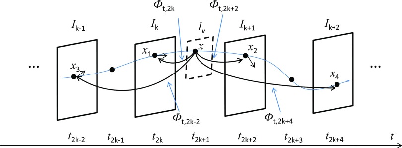
Assume that we have an image sequence In(n = 0, 1, 2, …, Nf). We define a flow of diffeomorphisms ϕ(x, t), t ∈ [0, Nf], x ∈ Ω⊂Rd(d = 2, 3) with smooth velocity field using the differential equation . We use Ns time steps for the velocity field between each two consecutive frames. Figure 1 shows the principle of intensity consistency along the point trajectories at a random time point (For convenience of illustration, we explain our method by using Ns = 2 for an example, but the idea behind it is the same when other integers are used). Assume that in the image sequence a point x in a virtual plane Iv at t moves through four consecutive frames Ik−1, Ik, Ik+1, Ik+2(t ⊂ [k, k + 1]). We use the notation to indicate the transformation which maps x from t to . Then the trajectories of point x in the four consecutive frames are , , ,. Their intensity values , , , in the four frames should be preserved since they are from the same physical point. Theoretically, the point x at t can be replaced by any time point along the trajectory and the four frames can be extended to all image frames in the sequences.
Figure 1.
The intensity of a point along the trajectory should be preserved. The optimal velocity field should minimize the difference of evolving image , , , at time point . We use two time steps (Ns = 2) between each consecutive frames for illustration.
In our implementation, we consider up to four frames as a compromise of rich intensity consistency context and computational efficiency (at the beginning and end of the sequence, three images are considered). On the one hand, considering consistency between two frames before and after a time point gives us reasonable temporal constraints on the point trajectories. On the other hand, consideration of more frames produces correspondence ambiguity due to speckle decorrelation. We define an energy term to measure the ICE as
| (3) |
The ICE function at time point t measures consistency of the intensity values of local frames under a velocity field. The optimal velocity field is estimated by minimizing a variational energy
| (4) |
with Nt = Ns*Nf being the total number of time points used in the velocity field. The first term regularizes the velocity field to make it spatiotemporally smooth, and the second term assures that the optimal velocity field minimizes the sum of the local intensity consistency error at all time points tk(k = 0, 1, 2, …, Nt).
We use an adaptive scheme to choose the value of Ns. It is initialized as 2. The B-spline parameters are checked at each iteration to make sure that the transformation between each two time points, i.e., , is diffeomorphic.66 If the condition is broken due to large deformation between two frames, the number of Ns will be doubled to tolerate larger deformation, while the transformation between time points is diffeomorphic.
Spatiotemporal velocity field regularization
In order to assure that ϕ(x, t) is diffeomorphic, we need to define to be spatiotemporally smooth under a differential operator L. The linear operator we choose is: , with ∇2(·) being a Laplacian operator, being the time derivative, and wt being a constant weight. In the discrete time form of velocity field, the first term of Eq. 4 is approximated by
| (5) |
with . The first term makes the velocity field spatially smooth, which is denoted as Esr. The second term keeps the particle velocity smooth and it is indicated by Etr. The overall effect is to make the velocity field spatiotemporally smooth.
Optimization
We use a steepest descent method to optimize the parameterized function. The derivative of the total registration energy with respect to the transformation parameters are calculated analytically.
Due to the fact that the ICE at each time point tk is made up of SSD functions of the three closest pairs of frames across it, the derivative of the ICE energy term in Eq. 4 with respect to the B-spline parameters is equalized to the sum of the derivative of the three SSD functions. Suppose we have two images I0 and I1, we want to estimate the derivative of SSD energy term at each tj with respect to a series of discrete velocity field B-spline parameters , with Ns the total number of time steps. We know from Sec. 2A that is only affected by the velocity field with j ⩽ k ⩽ Ns − 1, and ϕj, 0 is only related to with 0 ⩽ k ⩽ j − 1. If we denote ci,m;k as the m component (m ∈ {x, y, z}) of the ith B-spline parameter of , the derivative of E0,1(tj) with respect to ci,m;k is
| (6) |
with Ω′ being the local support of the B-spline kernel function, ∇m(·) being the mth component of the image gradient, and and being the derivative of the concatenated B-spline function with respect to the B-spline parameters which are calculated using chain rule.57, 65 By replacing image pair of I0 and I1 with the three pairs of images used in intensity consistency error at each tk, we get the derivative of the total similarity metric with respect to the velocity field parameters.
For the derivative of the spatial and temporal regularization energies with respect to ci,m;k, we have
| (7) |
with being the second derivative of the B-spline function with respect to m component. Considering that the displacement between two time steps is small, we have
| (8) |
The registration energy can be optimized by starting from initial position and descending along the negative gradient direction at each iteration until there is no significant decrease.
Implementation
In our experiments, we used a series of B-spline transformations with grid spacing of 10 voxels in each dimension to represent the velocity field. The values of λ and wt were chosen to be 0.1 and 0.001 to allow the range of the ICE function and the regularization term to be comparable. The algorithm was implemented with Matlab67 under a Windows XP 64-bit system on an eight-core 2.13 GHz Xeon CPU machine with 30 GB RAM. For 2D image sequence of 11 frames with a size of 274 × 192, it took about 10 min to estimate the motion with single core computing. For 3D sequences, the most frequently called functions such as the 3D B-spline interpolation of the displacement field and the trilinear interpolation of the image have been implemented by using OpenMP (Ref. 68) to effectively support the multicore processors. The typical execution time for a 3D sequence of 15 frames with frame size of 137 × 96 × 124 was about 2 h.
EXPERIMENTS AND DATASETS
We use simulated datasets and images of an ex vivo rabbit heart phantom, in vivo open-chest pig heart datasets, and human echocardiographic sequences to validate our method.
Simulated datasets
Both 2D and 3D sequences were generated in the simulated data experiments. In 2D test sequences, a long axis left ventricle (LV) ED frame with a size of 274 × 192 pixels was used as a reference frame. This frame was then deformed with a series of known continuous displacement field functions. The deformation was symmetric along the LV long axis to simulate the myocardial contraction along the radial and longitudinal directions. The displacement functions in x and y directions are defined as
| (9) |
| (10) |
with xc, rd being the short axis center coordinate and the average LV short axis radius, yapex and ybase being the height of base and apex, Nf and i being the number of frames and the frame index, and ax, ay being the magnitudes of displacement field which are the largest shift in axial and longitudinal directions. An image sequence with Nf + 1 frames (including the reference frame) was generated with i varying from 0 to Nf to simulate the motion in one cardiac cycle from ED to ES and then back to ED, where i = 0 corresponds to the reference frame itself. Three sequences each with 11 frames were simulated with multiplicative noise added to each frames. The noise was sampled from a uniform distribution with zero mean and variances 0.06, 0.08, and 0.10, respectively, for each image sequence. The gray level of the original reference frame was within [0,1] and that of each simulated frame was rescaled to [0,1] after adding noise. The magnitude parameters ax and ay were set to be 5 and 15, respectively. The reference frame with geometrical parameters for simulation and the 6th simulated frame with noise variance 0.10 are shown together with the ground truth displacement field in Fig. 2.
Figure 2.

The reference frame and the 6th frame in the variance 0.1 sequence and the ground truth displacement field.
In 3D test sequences, an ED volume frame was used as a reference. It was deformed with a spatiotemporal deformation, and a series of frames were generated. We assume that the LV short axis planes are parallel to xy coordinate plane and the long axis is along z direction. The displacement field functions fx, y in xy plane and fz in z direction are defined as
| (11) |
| (12) |
with (x, y, z) being the coordinate of each point, xp being the coordinate projected into xy plane, xc being the long axis projected in the xy plane, rd being the average radius of the LV short axis plane, being the unit vector from the short axis plane center pointing to xp, zapex, and zbase being the height of base and apex plane, Nf and i being the number of simulated frames and the frame index, and ax, ay being the magnitudes of displacement fields which are the largest deformation in radial and longitudinal directions. Three sequences with noise variances of 0.06, 0.08, 0.10 were simulated using the same noise model as in 2D experiments. The reference volume size is 137 × 96 × 124 voxels and number of frames is 11. The magnitude parameters axy and az are set to 5 and 6, respectively. Figure 3 shows the reference frame, 6th simulated frame, and the corresponding displacement fields in orthogonal slices of the sequence with noise variance of 0.1.
Figure 3.
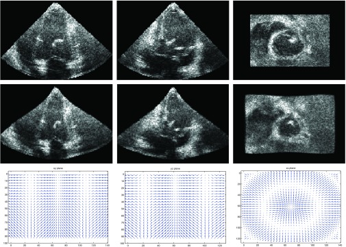
From the top to bottom, the first row shows the three orthogonal view of the reference frame (ED). The second row shows those of the 6th frame (ES). The third row shows the displacement fields in the orthogonal planes between these two frames.
Ex vivo rabbit heart phantom datasets
We validated our method with real datasets from rabbit heart phantom with sonomicrometers69 attached to the myocardial wall. Sonomicrometry, used as ground truth, is a method to measure the distance between the sono (piezoelectric) crystals based on the speed of acoustic signals through the medium they are embedded in. In this test, two sono crystals were implanted on the apical and mid myocardium of the phantom (Fig. 4). Freshly harvested rabbit hearts were used. A balloon was inserted into the phantom and connected to a pump which produced systole and diastole phases periodically. The stroke volume can be varied to control the deformation of the myocardium. It varied uniformly from 1ml to 5ml with 1 ml increment. The image sequences were acquired using Philips IU22 system with an X6-1 transducer. Each sequence had ten frames with frame size 109 × 129 × 129 and voxel size 0.57 mm3. The position of the crystals in the ED frame was manually located by a radiologist. Five sequences with varying stroke volume were acquired and the peak strain of the two crystals, which was defined as the largest relative displacement change to their initial distance within one heart cycle, were recorded with each sequence. We evaluated the two points peak strain by using our method and compared the estimated results with the sonomicrometry records.
Figure 4.

The three center orthogonal views of the ED frame of the rabbit model. The two points in the long axis view shows the location of the two sonomicrometers on the phantom myocardium.
In vivo open-chest pig heart datasets
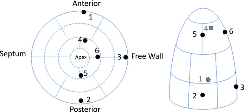
We validated our method with image sequences of two open-chest adult pigs with sonomicrometry. The image sequences were acquired using a Philips IE33 system with an X7 cardiac probe placed directly on the cardiac apex, separated by a small piece of fresh liver as standoff (2–4 cm). Sector width and depth were adjusted to allow inclusion of LV walls within the image region. For each pig, three sequences were acquired to study the LV motion under different steady states. The first sequence was the baseline under normal conditions. The second sequence was acquired, while the inferior vena cava (IVC) was occluded by a pneumatic occluder until the preload was dropped to the ED pressure level. The third sequence was a myocardial ischemia case which was captured after the left anterior descending (LAD) coronary artery was ligated for 5–7 min. The number of frames for each sequence varied from 13 to 21 and the typical frame size was 171 × 155 × 120 with voxel size of 0.836 mm3. The ED and ES frames of a baseline sequence are shown in Fig. 5 as an example. For the first pig, we implanted six sonomicrometers in the epicardium for validation of the tracking accuracy. Atraumatic surgical and fine suturing techniques were used to fix the crystals in the epicardium with minimal damage. All the experiments were approved by the OHSU Institutional Animal Care and Use Committee. Three crystals (S1–S3) were implanted on the myocardium in the short axis plane with 20% long axis height from the base, and the other three crystals (S4–S6) were implanted in the short axis plane which was in 80% long axis height (Fig. 6). The crystal positions in the ED frames were manually located by a radiologist and their positions in other frames were propagated by the estimated transformation. The relative coordinates of the six crystals with one as the reference varied with time, and were recorded by sonomicrometry. The distance between crystals measured in the sonomicrometry was used as ground truth to compare with that estimated from the echocardiography.
Figure 5.
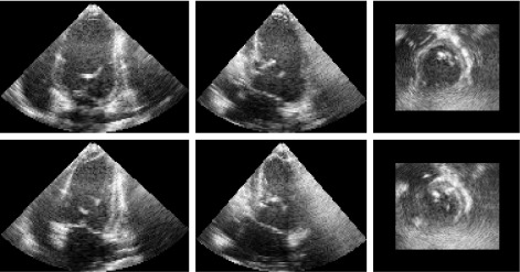
The real pig baseline dataset. The top row shows the orthogonal views of the end-diastole frame. The bottom row shows those of the end-systole frame.
Figure 6.
The locations of six crystals on the myocardium.
Human datasets
We used the image sequences from an open access database for motion tracking.70 The 3D echocardiography sequences of 15 healthy subjects were acquired by using an IE33 system with an X3-1 transducer. The typical frame size was 208 × 224 × 208 with voxel size 0.82 × 0.82 × 0.72 mm and the number of frames varied from 11 to 24. For each subject, a 3D tagged MRI sequence was also acquired by using a 3T Philips Achieva system. Twelve landmarks were tracked in the tagged MRI sequences by two expert observers. The landmarks in the tagged MRI were then transformed into the 3D echocardiography coordinate by using point based registration (Fig. 7). The transformed tagged MRI landmarks were then used as ground truth to validate the estimated motion from echocardiography. Fifteen subjects were used for our validation (V1–V16, V3 was not included).
Figure 7.

The three orthogonal view of ED frame of one subject and the 12 landmark positions from one expert observer.
RESULTS
We compared our method with two recently developed diffeomorphic motion estimation methods. The first one is a diffeomorphic B-spline method with transformation transitivity as a temporal constraint. The constraint ensures that in each three consecutive frames, the composition of the transformations obtained from each two consecutive frame registrations is equal to the transformation from the first frame to the third one.51 We refer to it as the transformation transitivity constraint (TTC) method. The second one is the temporal diffeomorphic free form deformation (TDFFD) method, which optimizes a spatiotemporal B-spline velocity field function by minimizing the SSD between the reference to each of the unwarped subsequent frames.58 The same regularization parameters were used for our method and the TTC method. For the TDFFD method, identical spatial spacing of B-spline was used in the 4D velocity field, and the temporal spacing was equal to the time step between two consecutive frames. All three methods were compared in the simulated datasets. In the rabbit heart dataset, we compared all the three methods with sonomicrometry. In the open-chest pig and human volunteer experiments, we compared our method with the TDFFD method since they were found to have closer performance.
Simulated datasets
We compared our method with TTC and TDFFD methods by tracking the trajectories of the points on the myocardium during the motion process. For 2D sequences, we used a region of interest in the myocardium as an example to show the tracking results. The region of interest is displayed as a green rectangle in the left figure of Fig. 2. Figure 8 shows the 11-frame trajectories of nine tracked points in this region for the sequence with noise variance of 0.06. The ground truth trajectories are overlaid for comparison. We can see, generally, that coordinates of the points in each time step in our method are closer to the ground truth. Larger errors can be seen in the right part of the trajectories in the TTC method. In the TDFFD method, larger errors appear in time steps near the end of the trajectories. We use the SSD between the estimated displacement fields and the ground truth in each frame to evaluate the transformation estimation errors. We show an example in Fig. 9 of the errors in both x and y coordinates in the sequence with noise variance of 0.08. We can see both the mean and variance in x and y directions in our method are smaller than the other two methods.
Figure 8.
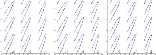
Trajectories of nine points in 11 frames in TTC method (left), TDFFD method (middle), and our method (right) (A rectangle shows the bounding box of these nine points in Fig. 2.) The ground truth trajectories are overlaid with the estimated curves for comparison. The arrow shows the velocity at each time step.
Figure 9.
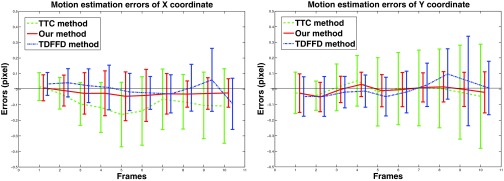
The motion estimation errors (mean and std unit in pixel) in x (left) and y (right) coordinates in the TTC method (dashed line), TDFFD method (dash-dot line), and our method (solid line).
We calculated the mean magnitude of transformation errors in the sequences of three noise variance using the three methods. In our method, the errors were 0.225, 0.267, and 0.312, while in the TTC method and the TDFFD method they were 0.329, 0.365, 0.403, and 0.314, 0.347, 0.392, respectively.
For 3D datasets, we show in Fig. 10 the errors in x, y, and z coordinates, for the sequence of noise variance 0.06. We can see that the variance of the error becomes larger toward the end of the sequence in the TTC method. In the TDFFD method, the means of the transformation estimation errors in three coordinates increase, which means the results were biased toward the reference frame. In our method, the mean and variance of the transformation estimation error change smoothly with the frame number. The average transformation estimation errors at three noise levels were 0.255, 0.274, 0.293 in our method and 0.322, 0.354, 0.391 in the TTC method and 0.279, 0.301, 0.325 in the TDFFD method.
Figure 10.

The transformation estimation errors (mean and std unit in voxel) of x (left), y(middle), and z (right) coordinates in the TTC method (dashed line), TDFFD method (dash-dot line), and our method (solid line) in each frame.
Ex vivo rabbit phantom datasets
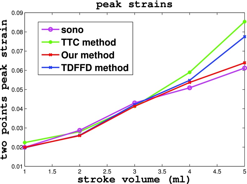
In the rabbit phantom test, the two point strain of the crystals in five echocardiography sequences with stroke volume uniformly varying from 1 ml to 5 ml were estimated and compared with those of the sonomicrometry. Figure 11 shows the two point strains varying in a cardiac cycle under different stroke volumes by sonomicrometry, TTC, TDFFD, and our method. We can see that two point strains curve from our method were closer to the ground truth of sonomicrometry than were those from the TTC and TDFFD methods. Figure 12 shows the estimated two point peak strains varying with the stroke volume in sonomicrometry, TTC, TDFFD, and our method. We can also see that our method has closer two point peak strains with sonomicrometry, especially in the sequence with stroke volume 5 ml.
Figure 11.
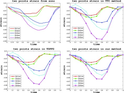
Two point strain varying with time under different stroke volume from sonomicrometry (top left), TTC method (top right), TDFFD method (bottom left), and our method (bottom right).
Figure 12.
The two point peak strains under different stroke volume estimated from sonomicrometry, TTC method, TDFFD method, and our method.
In vivo open-chest pig heart datasets
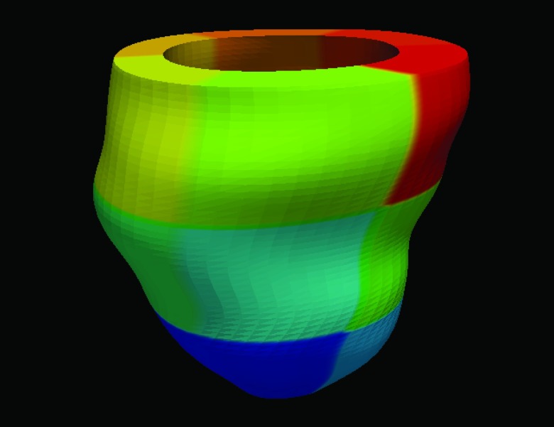
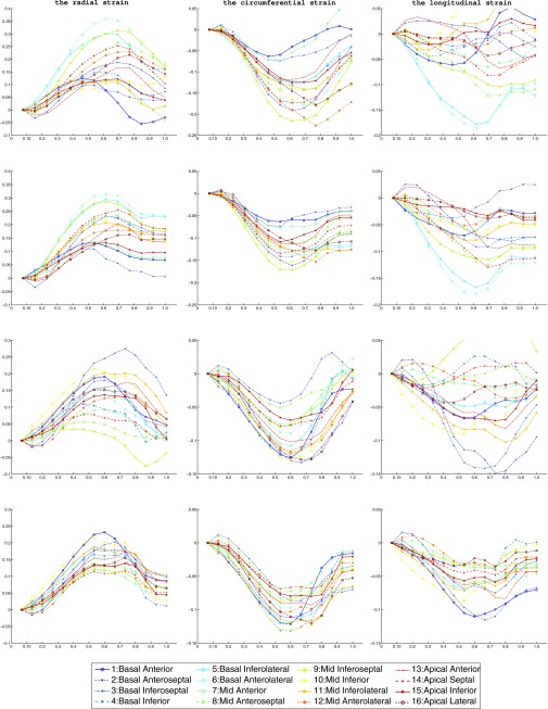
For the in vivo open-chest pig heart datasets, we compared strain derived from our method with that from the TDFFD method. We use the Green-Lagrangian strain71 which measures how much the displacement function varies locally in a given direction. The myocardium strains were evaluated along the radial, circumferential, and longitudinal directions by using the transformation obtained.6 We developed a program which can semiautomatically label the endocardium and epicardium contours in the short axis image planes between the mitral valve and the apex. For each contour, a closed curve parameterized by cubic B-spline was fitted to the manually picked boundary points around the myocardium. The contours were then resampled uniformly by a constant number of points along them. The endocardium and the epicardium surfaces were generated by connecting all their contours using triangles. Each vertex in both endocardium and epicardium was then assigned a segment attribute. We used the AHA myocardium segments convention72 and the strains of 16 myocardium segments were evaluated as the average strain in each segment. The 17th (apex) segment was excluded because the directions were usually unstable. An example for the 16 AHA segments is shown in Fig. 13. The radial, circumferential, and longitudinal strains of the two baseline sequences are shown in Fig. 14. From the strain plots, we can see the motion consistency between segments is improved in our method. In the TDFFD method, the estimated strains after ES are more divergent. This is due to the larger intensity variations between the reference image with distant frames. As a result, the displacement fields obtained have larger estimation errors.
Figure 13.
An illustration of the 16 AHA segments.
Figure 14.
The radial, circumferential, and longitudinal strains of the 16 AHA segments in the TDFFD method (first and third rows) and our method (second and fourth rows) estimated from two baseline sequences. The horizontal axis is the normalized cardiac time, the vertical axis is the strain. The markers used for the 16 AHA segments are shown in the bottom of the figure.
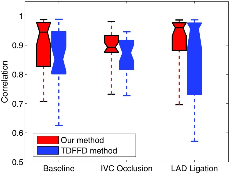
We compared the performance of the two algorithms by computing the correlations between the time varying functions of estimated pairwise distances from echo and those from sonomicrometry. The results for the baseline, IVC occlusion, and LAD ligation sequences are shown in Tables 1, 2, 3 respectively. Numbers S1–S6 are the indices of the sono crystals. Each table entry shows the correlation of the time function of pairwise crystal distance from sonomicrometry with that estimated from echo in the TDFFD (left side) and our method (right side). We can see that most of the correlation values are improved in our method in all three steady states. The box plots of the correlation values in the proposed and TDFFD methods for the three steady states are shown in Fig. 15. The increase of the average correlations in our method than TDFFD method is more than 5% for our datasets.
Table 1.
The correlations between the estimated pairwise distances and those from the sonomicrometry, with TDFFD method (numbers to the left), and our method (numbers to the right) in the baseline sequence. Numbers S1–S6 index the six sonomicrometry markers.
| S1 | S2 | S3 | S4 | S5 | S6 | |
|---|---|---|---|---|---|---|
| S1 | 1.0/1.0 | 0.807/0.707 | 0.710/0.968 | 0.834/0.970 | 0.802/0.881 | 0.950/0.967 |
| S2 | 0.807/0.707 | 1.0/1.0 | 0.780/0.726 | 0.946/0.979 | 0.823/0.929 | 0.907/0.828 |
| S3 | 0.710/0.968 | 0.780/0.726 | 1.0/1.0 | 0.928/0.988 | 0.852/0.928 | 0.960/0.978 |
| S4 | 0.834/0.970 | 0.946/0.979 | 0.928/0.988 | 1.0/1.0 | 0.989/0.981 | 0.855/0.945 |
| S5 | 0.802/0.881 | 0.823/0.929 | 0.852/0.928 | 0.989/0.981 | 1.0/1.0 | 0.625/0.727 |
| S6 | 0.950/0.967 | 0.907/0.828 | 0.960/0.978 | 0.855/0.945 | 0.625/0.727 | 1.0/1.0 |
Table 2.
The correlations between the estimated pairwise distances and those from the sonomicrometry, with TDFFD method (numbers to the left) and our method (numbers to the right) in the IVC occlusion sequence. Numbers S1–S6 index the six sonomicrometry markers.
| S1 | S2 | S3 | S4 | S5 | S6 | |
|---|---|---|---|---|---|---|
| S1 | 1.0/1.0 | 0.857/0.955 | 0.874/0.841 | 0.853/0.928 | 0.759/0.891 | 0.906/0.880 |
| S2 | 0.857/0.955 | 1.0/1.0 | 0.727/0.810 | 0.946/0.976 | 0.913/0.927 | 0.817/0.876 |
| S3 | 0.874/0.841 | 0.727/0.810 | 1.0/1.0 | 0.932/0.933 | 0.856/0.889 | 0.890/0.893 |
| S4 | 0.853/0.928 | 0.946/0.976 | 0.932/0.933 | 1.0/1.0 | 0.917/0.898 | 0.921/0.981 |
| S5 | 0.759/0.891 | 0.913/0.927 | 0.856/0.889 | 0.917/0.898 | 1.0/1.0 | 0.760/0.732 |
| S6 | 0.906/0.880 | 0.817/0.876 | 0.890/0.893 | 0.921/0.981 | 0.760/0.732 | 1.0/1.0 |
Table 3.
The correlations between the estimated pairwise distances and those from the sonomicrometry, with TDFFD method (numbers to the left), and our method (numbers to the right) in the LAD ligation sequence. Numbers S1–S6 index the six sonomicrometry markers.
| S1 | S2 | S3 | S4 | S5 | S6 | |
|---|---|---|---|---|---|---|
| S1 | 1.0/1.0 | 0.972/0.975 | 0.967/0.977 | 0.731/0.870 | 0.987/0.986 | 0.979/0.960 |
| S2 | 0.972/0.975 | 1.0/1.0 | 0.826/0.882 | 0.957/0.976 | 0.640/0.824 | 0.571/0.696 |
| S3 | 0.967/0.977 | 0.826/0.882 | 1.0/1.0 | 0.963/0.981 | 0.829/0.935 | 0.630/0.901 |
| S4 | 0.731/0.870 | 0.957/0.976 | 0.963/0.981 | 1.0/1.0 | 0.976/0.981 | 0.979/0.986 |
| S5 | 0.987/0.986 | 0.640/0.824 | 0.829/0.935 | 0.976/0.981 | 1.0/1.0 | 0.926/0.919 |
| S6 | 0.979/0.960 | 0.571/0.696 | 0.630/0.901 | 0.979/0.986 | 0.926/0.919 | 1.0/1.0 |
Figure 15.
The box plots of the correlation values in our method and the TDFFD method for the baseline, IVC occlusion, and LAD ligating cases. The bottom and top box boundary and the center line show the first quantile, third quantile, and median, respectively. The ends of the whiskers show the minimum and maximum of each case. For each dataset in each method 30 correlation values are averaged, except the six diagonal correlation value which is one.
Human datasets
We used the landmarks labeled by one observer as ground truth and the target registration error73 was used for the validation of tracking errors. The target registration error of the 12 landmarks in the ES and the last frames were evaluated in our experiments.74, 75 We compared our method with the modified TDFFD method which used the weighted first-to-following and frame-to-frame similarity measurements. We also evaluated the results from a frame-to-frame method for comparison. The tracking errors in the three methods are shown in Fig. 16. Our method generally has smaller average tracking error and variance than the TDFFD method and the frame-to-frame method.
Figure 16.
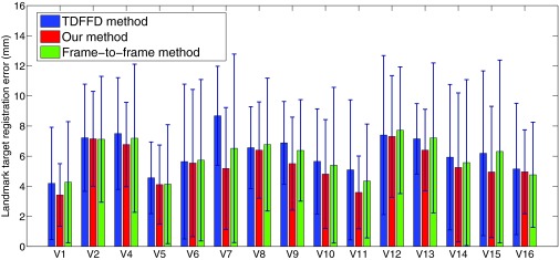
The tracking error (mean and std) of the seven subjects in the TDFFD method, our method, and the frame-to-frame method.
DISCUSSION AND CONCLUSION
We proposed a diffeomorphic motion estimation method with temporal smoothness by constraining the velocity field to have maximum local intensity consistency within multiple image frames. Simulated and real cardiac sequences tests showed that results using our method are more accurate than other competing temporal diffeomorphic methods. Tests with sonomicrometry showed that the tracked crystal positions have good consistency with the ground truth and our method has higher accuracy than the TDFFD method. Validation with an open access human cardiac dataset showed that our method has smaller feature tracking errors than both TDFFD and frame-to-frame methods. From the human cardiac dataset test, we see that even when a weighted frame-to-frame and first-to-following similarity measurement is used, the dissimilarity between distant frames may cause larger feature tracking errors.
Our method extends the frame-to-frame motion estimation method to multiple frames. With more frames included into the similarity measurement, the similarity is more robust against noise than the frame-to-frame method. Furthermore, the ICE similarity measurement is defined on multiple time points between four consecutive frames, to allow the four frames unwarped to this time point to be as similar as possible. At each time point, the estimated spatiotemporal transformation maximizes the similarity of the four consecutive frames around it. The transformation is consistent with two frames before and after it while preserving good temporal smoothness. This introduces more intensity consistency for the spatiotemporal transformation than the frame-to-frame method and the TDFFD method.
One factor to consider is the number of consecutive frames to include in ICE. This will vary for different types of data, and will depend on several factors, such as the level of decorrelation from frame to frame and computation load. Inclusion of distant frames introduces uncorrelated intensity into similarity measurements. If only two frames are considered (the frame-to-frame case), the transformation errors tend to accumulate faster because the transformation parameters are only estimated by optimizing the similarity of two consecutive frames, instead of optimizing a groupwise similarity measurement. In this sense, more frames will be beneficial. In addition, more frames will lead to better temporal consistency. However, inclusion of more frames will increases the computation time. In our test, we use four frames as a compromise of these factors.
Our future research topics include the study of region-based intensity consistency between consecutive frames, and the design of improved groupwise similarity measurement.
ACKNOWLEDGMENTS
This paper is supported by a NIH/NHLBI Grant No. 1R01HL102407-01 awarded to Xubo Song and David Sahn.
References
- Sherry L. M., Xu J. Q., and Kenneth D. K., “Deaths: Final data for 2010,” National Vital Statistics Reports No. 61, 2013. [PubMed]
- Bijnens B., Claus P., Weidemann F., Strotmann J., and Sutherland G. R., “Investigating cardiac function using motion and deformatio analysis in the setting of coronary artery disease,” Circulation 116, 2453–2464 (2007). 10.1161/CIRCULATIONAHA.106.684357 [DOI] [PubMed] [Google Scholar]
- Buckberg G., Hoffman J. I. E., Mahajan A., Saleh S., and Coghlan C., “Cardiac mechanics revisited the relationship of cardiac architecture to ventricular function,” Circulation 118, 2571–2587 (2008). 10.1161/CIRCULATIONAHA.107.754424 [DOI] [PubMed] [Google Scholar]
- Axel L., “Biomechanical dynamics of the heart with MRI,” Annu. Rev. Biomed. Eng. 4, 321–347 (2002). 10.1146/annurev.bioeng.4.020702.153434 [DOI] [PubMed] [Google Scholar]
- Kiss G., Barbosa D., Hristova K., Crosby J., Orderud F., Claus P., Amundsen B., Loeckx D., D’hooge J., and Torp H. G., “Assessment of regional myocardial function using 3D cardiac strain estimation: Comparison against conventional echocardiographic assessment,” in IEEE International Ultrasonics Symposium (IUS) (IEEE, Rome, 2009), pp. 507–510.
- Elen A., Choi H. F., Loeckx D., Gao H., Claus P., Suetens P., Maes F., and D’hooge J., “Three-dimensional cardiac strain estimation using spatio-temporal elastic registration of ultrasound images: A feasibility study,” IEEE Trans. Med. Imaging 27(11), 1580–1591 (2008). 10.1109/TMI.2008.2004420 [DOI] [PubMed] [Google Scholar]
- Mäkelä T., Clarysse P., Sipilä O., Pauna N., Pham Q. C., Katila T., and Magnin I. E., “A review of cardiac image registration methods,” IEEE Trans. Med. Imaging 21(9), 1011–1021 (2002). 10.1109/TMI.2002.804441 [DOI] [PubMed] [Google Scholar]
- Bertini M., Sengupta P. P., Nucifora G., Delgado V., Ng C. T., Marsan N. A., Shanks M., van B. R. J., Schalij M. J., Narula J., and Bax J. J., “Role of left ventricular twist mechanics in the assessment of cardiac dyssynchrony in heart failure,” JACC 2(12), 1425–1435 (2009). 10.1016/j.jcmg.2009.09.013 [DOI] [PubMed] [Google Scholar]
- Lang R. M., Goldstein S. A., Kronzon I., and Khandheria B. K., Dynamic Echocardiography (Elesvier, St. Louis, MO, 2010). [Google Scholar]
- Axel L., Montillo A., and Kim D., “Tagged magnetic resonance imaging of the heart: A survey,” Med. Imag. Anal. 9(4), 376–393 (2005). 10.1016/j.media.2005.01.003 [DOI] [PubMed] [Google Scholar]
- Ohnesorge B. M., Becker C. R., Flohr T. G., and Reiser M. F., Multi-Slice CT in Cardiac Imaging: Technical Principles, Clinical Applications and Future Developments (Springer, New York, 2002). [Google Scholar]
- Mondillo S., Galderisi M., Mele D., Cameli M., Lomoriello V. S., Zaca V., Ballo P., Andrea A. D., Muraru D., Losi M., Agricola E., ’Errico A. D., Buralli S., Sciomer S., Nistri S., and Badano L., “Speckle-tracking echocardiography a new technique for assessing myocardial function,” J. Ultrasound Med. 30(1), 71–83 (2011). [DOI] [PubMed] [Google Scholar]
- Geyer H., Caracciolo G., Abe H., Wilansky S., Carerj S., Gentile F., Nesser H. J., Khandheria B., Narula J., and Sengupta P. P., “Assessment of myocardial mechanics using speckle tracking echocardiography: Fundamentals and clinical applications,” J. Am. Soc. Echocardiogr. 23(4), 351–369 (2010). 10.1016/j.echo.2010.02.015 [DOI] [PubMed] [Google Scholar]
- Ho C. Y. and Solomon S. D., “A clinician's guide to tissue doppler imaging,” Circulation 113, e396–e398 (2006). 10.1161/CIRCULATIONAHA.105.579268 [DOI] [PubMed] [Google Scholar]
- Park J., Metaxas D., Young A. A., and Axel L., “Deformable models with parameter functions for cardiac motion analysis from tagged MRI data,” IEEE Trans. Med. Imaging 15(3), 278–289 (1996). 10.1109/42.500137 [DOI] [PubMed] [Google Scholar]
- Park J., Metaxas D. N., and Axel L., “Analysis of left ventricular wall motion based on volumetric deformable models and MRI SPAMM,” Med. Image Anal. 1(1), 53–72 (1996). 10.1016/S1361-8415(01)80005-0 [DOI] [PubMed] [Google Scholar]
- Papademetris X., Sinusas A. J., Dione D. P., and Duncan J. S., “Estimation of 3D left ventricular deformation from echocardiography,” Med. Imag. Anal. 5(1), 17–28 (2001). 10.1016/S1361-8415(00)00022-0 [DOI] [PubMed] [Google Scholar]
- Frangi A. F., Niessen W. J., and Viergever M. A., “Three-dimensional modeling for functional analysis of cardiac images: A review,” IEEE Trans. Med. Imaging 20(1), 2–25 (2001). 10.1109/42.906421 [DOI] [PubMed] [Google Scholar]
- Rueckert D., Sonoda L. I., Hayes C., Hill D. L. G., Leach M. O., and Hawkes D. J., “Nonrigid registration using free-form deformations: Application to breast MR images,” IEEE Trans. Image Process. 18(8), 712–721 (1999). 10.1109/42.796284 [DOI] [PubMed] [Google Scholar]
- Thirion J. P., “Image matching as a diffusion process: An analogy with Maxwell's demons,” Med. Imag. Anal. 2(3), 243–260 (1998). 10.1016/S1361-8415(98)80022-4 [DOI] [PubMed] [Google Scholar]
- Cachier P., Bardinet E., Dormont D., Pennec X., and Ayache N., “Iconic feature based nonrigid registration: The PASHA algorithm,” J. Comput. Vis. Image Understand. 89(2–3), 272—298 (2003). 10.1016/S1077-3142(03)00002-X [DOI] [Google Scholar]
- Beauchemin S. S. and Barron J. L., “The computation of optical flow,” J. ACM Comput. Surv. 27(3), 433–466 (1995). 10.1145/212094.212141 [DOI] [Google Scholar]
- Christensen G. E., Rabbit R. D., and Miller M. I., “Deformable templates using large deformation kinematics,” IEEE Trans. Image Process. 5(10), 1435–1447 (1996). 10.1109/83.536892 [DOI] [PubMed] [Google Scholar]
- Hermosillo G., Chefd’Hotel C., and Faugeras O., “Variational methods for multimodal image matching,” Int. J. Comput. Vis. 50(3), 329–343 (2002). 10.1023/A:1020830525823 [DOI] [Google Scholar]
- Myronenko A., Song X. B., and David J. S., “LV motion tracking from 3D echocardiography using textural and structural information,” in Proceedings of MICCAI, Lecture Notes in Computer Science Vol. 4792 (Springer, Heidelberg, 2007), pp. 428–435. [DOI] [PubMed]
- Chandrashekara R., Mohiaddin R. H., and Rueckert D., “Analysis of 3-D myocardial motion in tagged MR images using nonrigid image registration,” IEEE Trans. Med. Imaging 23(10), 1245–1250 (2004). 10.1109/TMI.2004.834607 [DOI] [PubMed] [Google Scholar]
- Mansi T., Peyrat J. M., Sermesant M., Delingette H., Blanc J., Boudjemline Y., and Ayache N., “Physically-constrained diffeomorphic demons for the estimation of 3D myocardium strain from cine-MRI,” in Proceedings of Functional Imaging and Modeling of the Heart, Lecture Notes in Computer Science Vol. 5528 (Springer, Heidelberg, 2009), pp. 201–210.
- Suhling M., Arigovindan M., Jansen C., Hunziker P., and Unser M., “Myocardial motion analysis from B-mode echocardiograms,” IEEE Trans. Image Process. 14(4), 525–536 (2005). 10.1109/TIP.2004.838709 [DOI] [PubMed] [Google Scholar]
- Rougon N., Petitjean C., Preteux F., Cluzel P., and Grenier P., “A non-rigid registration approach for quantifying myocardial contraction in tagged MRI using generalized information measures,” Med. Image Anal. 9(4), 353—375 (2005). 10.1016/j.media.2005.01.005 [DOI] [PubMed] [Google Scholar]
- Boldea V., Sharp G. C., Jiang S. B., and Sarrut D., “4D-CT lung motion estimation with deformable registration: Quantification of motion nonlinearity and hysteresis,” Med. Phys. 35(3), 1008–1018 (2008). 10.1118/1.2839103 [DOI] [PubMed] [Google Scholar]
- Reinhardt J. M., Ding K., Cao K. L., Christensen G. E., Hoffman E. A., and Bodas S. V., “Registration-based estimates of local lung tissue expansion compared to xenon CT measures of specific ventilation,” Med. Image Anal. 12(6), 752–763 (2008). 10.1016/j.media.2008.03.007 [DOI] [PMC free article] [PubMed] [Google Scholar]
- Huang J., Abendschein D., Dávila-Román V. G., and Amini A. A., “Spatio-temporal tracking of myocardial deformation with a 4D B-spline model from tagged MRI,” IEEE Trans. Med. Imaging 18(10), 957–972 (1999). 10.1109/42.811299 [DOI] [PubMed] [Google Scholar]
- Bardinet E., Cohen L. D., and Ayache N., “Dynamic 3D models with global and local deformations: Deformable superquadrics,” IEEE Trans. Pattern Anal. Mach. Intell. 13(9), 703–714 (1991). 10.1109/34.85659 [DOI] [Google Scholar]
- Bardinet E., Cohen L. D., and Ayache N., “Tracking and motion analysis of the left ventricle with deformable superquadrics,” Med. Imag. Anal. 1(2), 129–149 (1996). 10.1016/S1361-8415(96)80009-0 [DOI] [PubMed] [Google Scholar]
- Montagnat J. and Delingette H., “4D deformable models with temporal constraints: Application to 4D cardiac image segmentation,” Med. Image Anal. 9(1), 87–100 (2005). 10.1016/j.media.2004.06.025 [DOI] [PubMed] [Google Scholar]
- Schaerera J., Casta C., Pousina J., and Claryssea P., “A dynamic elastic model for segmentation and tracking of the heart in MR image sequences,” Med. Image Anal. 14(6), 738–749 (2010). 10.1016/j.media.2010.05.009 [DOI] [PubMed] [Google Scholar]
- Gerard O., Billon A. C., Rouet J. M., Jacob M., Fradkin M., and Allouche C., “Efficient model-based quantification of the left ventricular function in 3D echocardiography,” IEEE Trans. Med. Imaging 21(9), 1059–1068 (2002). 10.1109/TMI.2002.804435 [DOI] [PubMed] [Google Scholar]
- Metz C. T., Klein S., Schaap M., Walsum T., and Niessen W. J., “Nonrigid registration of dynamic medical imaging data using nD+t B-splines and a groupwise optimization approach,” Med. Imag. Anal. 15(2), 238–249 (2011). 10.1016/j.media.2010.10.003 [DOI] [PubMed] [Google Scholar]
- Wang Y., Georgescu B., Houle H., and Comaniciu D., “Volumetric myocardial mechanics from 3D+t ultrasound data with multi-model tracking,” in Proceedings of MICCAI Workshop of STACOM, Lecture Notes in Computer Science Vol. 6364 (Springer, Heidelberg, 2010), pp. 184–193.
- Comaniciu D., Zhou X., and Krishnan S., “Robust real-time tracking of myocardial border: An information fusion approach,” IEEE Trans. Med. Imaging 23(7), 849–860 (2004). 10.1109/TMI.2004.827967 [DOI] [PubMed] [Google Scholar]
- McEachen J. C., Nehorai A., and Duncan J. S., “Multiframe temporal estimation of cardiac nonrigid motion,” IEEE Trans. Image Process. 9(4), 651–665 (2000). 10.1109/83.841941 [DOI] [PubMed] [Google Scholar]
- Ledesma-carbayo M. J., Jan K., Manuel D., Andrés S., Sühling M., Hunziker P. R., and Unser M., “Spatio-temporal nonrigid registration for ultrasound cardiac motion estimation,” IEEE Trans. Med. Imaging 24(9), 1113–1126 (2005). 10.1109/TMI.2005.852050 [DOI] [PubMed] [Google Scholar]
- Yigitsoy M., Wachinger C., and Navab N., “Temporal groupwise registration for motion modeling,” in Proceedings of Information Processing in Medical Imaging, Lecture Notes in Computer Science Vol. 6801 (Springer, Heidelberg, 2011), pp. 648–659. [DOI] [PubMed]
- Delhay B., Clarysse P., and Magnin I. E., “Locally adapted spatio-temporal deformation model for dense motion estimation in periodic cardiac image sequences,” in Proceedings of Functional Imaging and Modeling of the Heart, Lecture Notes in Computer Science Vol. 4466 (Springer, Heidelberg, 2007), pp. 393–402.
- Peyat J. M., Delingette H., Sermesant M., Xu C. Y., and Ayache N., “Registration of 4D cardiac CT sequences under trajectory constraints with multichannel diffeomorphic demons,” IEEE Trans. Med. Imaging 29(7), 1351–1368 (2010). 10.1109/TMI.2009.2038908 [DOI] [PubMed] [Google Scholar]
- Perperidis D., Mohiaddin R. H., and Rueckert D., “Spatio-temporal free-form registration of cardiac MR image sequences,” Med. Image Anal. 9(5), 441—456 (2005). 10.1016/j.media.2005.05.004 [DOI] [PubMed] [Google Scholar]
- Castillo E., Castillo R., Martinez J., Shenoy M., and Guerrero T., “Four-dimensional deformable image registration using trajectory modeling,” Phys. Med. Biol. 55(1), 305–327 (2010). 10.1088/0031-9155/55/1/018 [DOI] [PMC free article] [PubMed] [Google Scholar]
- Vandemeulebroucke J., Rit S., Kybic J., Clarysse P., and Sarrut D., “Spatiotemporal motion estimation for respiratory-correlated imaging of the lungs,” Med. Phys. 38(1), 166–178 (2011). 10.1118/1.3523619 [DOI] [PubMed] [Google Scholar]
- Sundar H., Littb H., and Shen D. G., “Estimating myocardial motion by 4D image warping,” Pattern Recog. 42(11), 2514–2526 (2009). 10.1016/j.patcog.2009.04.022 [DOI] [PMC free article] [PubMed] [Google Scholar]
- Klein G. J. and Huesman R. H., “Four-dimensional processing of deformable cardiac PET data,” Med. Image Anal. 6(1), 29–46 (2002). 10.1016/S1361-8415(01)00050-0 [DOI] [PubMed] [Google Scholar]
- Skrinjar O., Bistoquet A., and Tagare H., “Symmetric and transitive registration of image sequences,” Int. J. Biomed. Imaging Hindawi, Cairo (2008). 10.1155/2008/686875 [DOI] [PMC free article] [PubMed] [Google Scholar]
- Beg M. F., Miller M. I., Trouve A., and Younes L., “Computing large deformation metric mappings via geodesic flows of diffeomorphisms,” Int. J. Comput. Vis. 61(2), 139–157 (2005). 10.1023/B:VISI.0000043755.93987.aa [DOI] [Google Scholar]
- Vercauteren T., Pennec X., Perchant A., and Ayache N.,“Diffeomorphic demons: Efficient non-parametric image registration,” NeuroImage 45(S1), S61–S72 (2009). 10.1016/j.neuroimage.2008.10.040 [DOI] [PubMed] [Google Scholar]
- Qiu A. Q., Albert M., Younes L., and Miller M. I., “Time sequence diffeomorphic metric mapping and parallel transport track time-dependent shape changes,” NeuroImage 45(S1), S51–S60 (2009). 10.1016/j.neuroimage.2008.10.039 [DOI] [PMC free article] [PubMed] [Google Scholar]
- Durrleman S., Pennec X., Trouv A., Braga J., Gerig G., and Ayache N., “Toward a comprehensive framework for the spatiotemporal statistical analysis of longitudinal shape data,” Int. J. Comput. Vis. 103(1), 22–59 (2013). 10.1007/s11263-012-0592-x [DOI] [PMC free article] [PubMed] [Google Scholar]
- Khan A. R. and Beg M. F., “Representation of time-varying shapes in the large deformation diffeomorphic framework,” in Proceedings of the International Symposium on Biomedical Imaging (IEEE, Paris, 2008), pp. 1521–1524.
- Craene M. De, Camara O., Bijnens B. H., and Frangi A. F., “Large diffeomorphic FFD registration for motion and strain quantification from 3D-US sequences,” in Proceedings of Functional Imaging and Modeling of the Heart, Lecture Notes in Computer Science Vol. 5528, 437–446 (2009).
- Craene M. De, Piella G., Camaraa O., Duchateaua N., Silvae E., Doltrae A., D’hooge J., Brugadae J., Sitgese M., and Frangi A. F., “Temporal diffeomorphic free-form deformation: Application to motion and strain estimation from 3D echocardiography,” Med. Imag. Anal. 16(1), 427–450 (2012). 10.1016/j.media.2011.10.006 [DOI] [PubMed] [Google Scholar]
- Dupuis P. and Grenander U., “Variational problems on flows of diffeomorphisms for image matching,” Q. Appl. Math. LVI(3), 587–600 (1998). [Google Scholar]
- Bistoquet A., Oshinski J., and Skrinjar O., “Myocardial deformation recovery from cine MRI using a nearly incompressible biventricular model,” Med. Image Anal. 12(1), 69—85 (2008). 10.1016/j.media.2007.10.009 [DOI] [PubMed] [Google Scholar]
- Meunier J., “Tissue motion assessment from 3D echographic speckle tracking,” Phys. Med. Biol. 43(5), 1241–1254 (1998). 10.1088/0031-9155/43/5/014 [DOI] [PubMed] [Google Scholar]
- Zhang Z. J., Sahn D. J., and Song X. B., “Frame to frame diffeomorphic motion analysis from echocardiographic sequences,” in Proceedings of the MICCAI Workshop of Third Mathematical Foundation of Computational Anatomy (MFCA) (Inria, Paris, 2011), pp. 15–24.
- Zhang Z. J., Sahn D. J., and Song X. B., “Temporal diffeomorphic motion analysis from echocardiographic sequences by using intensity transitivity consistency,” in Proceedings of the Second International Conference on Statistical Atlases and Computational Models of the Heart: Imaging and modelling challenges (STACOM), Lecture Notes in Computer Science Vol. 7085 (Springer, Heidelberg, 2011), pp. 274–284.
- Beg M. F. and Khan A., “Symmetric data attachment terms for large deformation image registration,” IEEE Trans. Med. Imaging 26(9), 1179–1189 (2007). 10.1109/TMI.2007.898813 [DOI] [PubMed] [Google Scholar]
- Ashburner J., “A fast diffeomorphic image registration algorithm,” NeuroImage 38(1), 95–113 (2007). 10.1016/j.neuroimage.2007.07.007 [DOI] [PubMed] [Google Scholar]
- Rueckert D., Aljabar P., Heckemann R. A., Hajnal J. V., and Hammers A., “Diffeomorphic registration using B-splines,” in Proceedings of MICCAI’06, Lecture Notes in Computer Science Vol. 4191 (Springer, Heidelberg, 2006), pp. 702–709. [DOI] [PubMed]
- MATLAB version 7.11.0 (R2010b), The MathWorks Inc., Natick, MA, 2010.
- http://www.openmp.com.
- http://www.sonometrics.com.
- Tobon C.-Gomez, Craene M. D., McLeod K., Tautz L., Shi W. Z., Hennemuth A., Prakosa A., Wang H., Carr-White G., Kapetanakis S., Lutz A., Rasche V., Schaeffter T., Butakoff C., Friman O., Mansi T., Sermesant M., Zhuang X., Ourselin S., Peitgen H. O., Pennec X., Razavi R., Rueckert D., Frangi A. F., and Rhode K. S., “Benchmarking framework for myocardial tracking and deformation algorithms: An open access database,” Med. Imag. Anal. 17(6), 632–648 (2013). 10.1016/j.media.2013.03.008 [DOI] [PubMed] [Google Scholar]
- Fung Y. C., First Course in Continuum Mechanics (Springer, Prentice Hall, NJ, 2010). [Google Scholar]
- Cerqueira M. D., Weissman N. J., Dilsizian V., Jacobs A. K., Kaul S., Laskey W. K., Pennell D. J., Rumberger J. A., Ryan T., and Verani M. S., “Standardized myocardial segmentation and nomenclature for tomographic imaging of the heart: A statement for healthcare professionals from the cardiac imaging committee of the council on clinical cardiology of the American Heart Association,” Circulation 105, 539–542 (2002). 10.1161/hc0402.102975 [DOI] [PubMed] [Google Scholar]
- Fitzpatrick J. M. and West J. B., “The distribution of target registration error in rigid-body point-based registration,” IEEE Trans. Med. Imaging 20(9), 917–927 (2001). 10.1109/42.952729 [DOI] [PubMed] [Google Scholar]
- Young A. A., “Model tags: Direct three-dimensional tracking of heart wall motion from tagged magnetic resonance images,” Med. Image Anal. 3(4), 361–372 (1999). 10.1016/S1361-8415(99)80029-2 [DOI] [PubMed] [Google Scholar]
- Metz C., Baka N., Kirisli H., Schaap M., Walsum T. V., Klein S., Neefjes L., Mollet N., Lelieveldt B., Bruijne M. D., and Niessen W., “Conditional shape models for cardiac motion estimation,” in Proceedings of MICCAI, Lecture Notes in Computer Science Vol. 6361 (Springer, Heidelberg, 2010), pp. 452–459. [DOI] [PubMed]


