Abstract
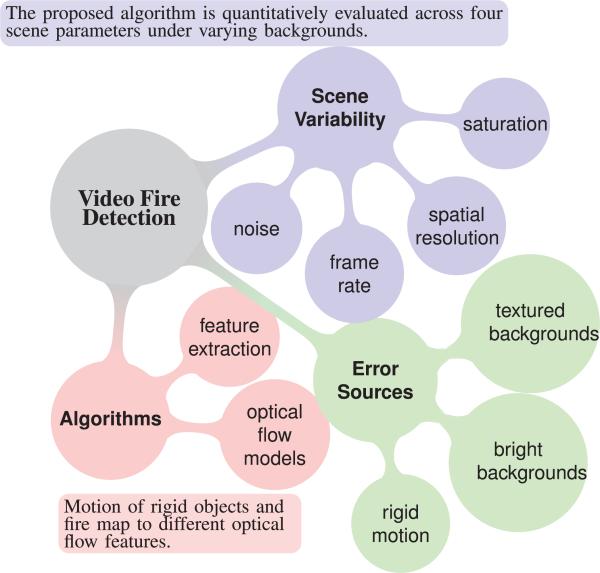
Computational vision-based flame detection has drawn significant attention in the past decade with camera surveillance systems becoming ubiquitous. Whereas many discriminating features, such as color, shape, texture, etc., have been employed in the literature, this paper proposes a set of motion features based on motion estimators. The key idea consists of exploiting the difference between the turbulent, fast, fire motion, and the structured, rigid motion of other objects. Since classical optical flow methods do not model the characteristics of fire motion (e.g., non-smoothness of motion, non-constancy of intensity), two optical flow methods are specifically designed for the fire detection task: optimal mass transport models fire with dynamic texture, while a data-driven optical flow scheme models saturated flames. Then, characteristic features related to the flow magnitudes and directions are computed from the flow fields to discriminate between fire and non-fire motion. The proposed features are tested on a large video database to demonstrate their practical usefulness. Moreover, a novel evaluation method is proposed by fire simulations that allow for a controlled environment to analyze parameter influences, such as flame saturation, spatial resolution, frame rate, and random noise.
Keywords: Fire detection, optical flow, optimal mass transport, video analytics
I. Introduction
Detecting the break-out of a fire rapidly is vital for prevention of material damage and human casualties.
This is a particularly serious problem in situations of congested automobile traffic, naval vessels, and heavy industry. Traditional point-sensors detect heat or smoke particles and are quite successful for indoor fire detection. However, they cannot be applied in large open spaces, such as hangars, ships, or in forests. This paper presents a video-detection approach geared toward these scenarios where point-sensors may fail. In addition to covering a wide viewing range, video cameras capture data from which additional information can be extracted; for example, the precise location, extent, and rate of growth. Surveillance cameras have recently become pervasive, installed by governments and businesses for applications like license-plate recognition and robbery deterrence. Reliable vision-based fire detection can feasibly take advantage of the existing infrastructure and significantly contribute to public safety with little additional cost.
Scope
Vision-based detection is composed of the following three steps. Preprocessing (1) is necessary to compensate for known sources of variability, e.g., camera hardware and illumination. Feature extraction (2) is designed for the detection of a specific target; a computation maps raw data to a canonical set of parameters to characterize the target. Classification algorithms (3) use the computed features as input and make decision outputs regarding the target's presence. Supervised machine-learning-based classification algorithms such as neural networks (NN) are systematically trained on a data set of features and ground truth.
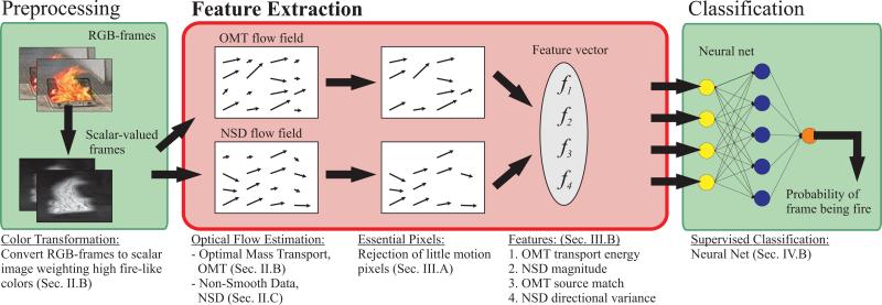
The scope of this paper is illustrated in Fig. 1. While aspects of preprocessing (1) and classification (3) are considered, the paper focuses on feature extraction (2): Motivated by physical properties of fire, a set of novel optical flow features are designed for vision-based fire detection.
Fig. 1.
A Visual outline of the scope of this paper. The underlying goal of the research is improved robustness to rigid motion of fire-colored objects and unfavorable backgrounds, which tend to cause many false detections in current systems.
Previous Work
Computer vision concepts are often inspired by human vision. A comprehensive and elegant description of the human perception of fire was presented by the 16th century French poet Du Bartas [1]: “Bright-flaming, heat-full fire, the source of motion.” Whereas Du Bartas missed the characteristic reddish color that almost any vision-based detection algorithm builds upon, e.g., [2], his quote covers most of the other features employed by previous methods. High brightness or luminance causes image pixels to saturate–one feature utilized in [3]–[5]. The instantaneous flame-like texture or spatial pattern are used in [4], [6], [7]. Features related to the flame's shape and change of shape are found in [3], [6], [7]. Also, the flickering, typical of fire, presents a popular feature [3], [4], which has also been analyzed in the wavelet domain [8], [9]. This paper is restricted to studying images in the visible spectrum and emitted heat or infrared light is not considered, but it is used in a number of approaches where infrared sensors are available [10]. Lastly, fire motion offers a whole suite of possible features. The authors of [11] consider the temporal variation of pixel intensity for fixed pixel locations. More recently, [12] develops a more comprehensive statistical approach by computing covariances of image quantities on small blocks, thus making use of spatial and temporal patterns. These statistics are applied directly to the image data and these methods are therefore comparably efficient. Optical flow estimators, on the other hand, transform the image sequence into estimated motion fields, allowing for a more insightful extraction of features. Classical optical flow algorithms are analyzed in [13] for the recognition of various dynamic textures.
Contribution
The contributions of this paper are: First, since classical optical flow methods are based on assumptions, e.g., intensity constancy and flow smoothness, which are not met by fire motion, we derive two optical flow estimators specifically designed for the detection of fire; optimal mass transport exploits the dynamic texture of flames, whereas a non-smooth modification of classical optical flow models saturated flames with no dynamic texture. Second, a new set of optical flow features is presented for fire detection; these features characterize magnitude and directionality of motion vectors. Third, thorough analysis on real and synthetic data is performed; it demonstrates the features’ ability to reliably detect fire while rejecting non-fire, rigidly moving objects. Finally, a novel way to evaluate fire detectors using fire simulations is proposed; this method allows for the quantitative evaluation of scene variability such as flame saturation, spatial resolution, frame rate and noise.
The proposed research is different from recent work in dynamic texture analysis [13]–[16] in that our design of the motion estimators and features is geared to the detection of flames. See Table I for a comparison to [13], which employs classical optical flow methods for the recognition of different dynamic textures. In our work, the optical flow estimators are modified to model the properties of fire motion. In particular, a prior color transformation, plus non-smooth regularization and brightness conserving optical flow are proposed. In Section III-B, detailed discussions explain how the extracted features differ compared to [13]. As one major difference, we compute a spatial structure preserving feature based on a unique property of the optimal mass transport solution. Regarding classification results, [13] is not comparable to our work, since [13] only classifies between 26 particular instances of dynamic textures (each one representing one class), and not between the presence/ absence of an event (e.g., “fire”) among many videos. Moreover, the data in [13] is a specialized high quality database, whereas our data comes from mass market and surveillance cameras.
TABLE I.
Comparison to Dynamic Texture Recognition [13]
| Fazekas et al. [13] | Our Work | |
|---|---|---|
| Optical Flow | Standard | Target-specific |
| Features | Spatially averaged, from one flow field | Structure preserving, from two flow fields |
| Classification | Recognition of textures | Detection of flames |
| Video Type | Specialized (high quality) | Mass market cameras |
Brightness conserving optical flow formulations have been employed in dynamic texture segmentation tasks [15], [16], but no attempt was made in classifying them, e.g., as fire, water, etc., using brightness conserving methods. Moreover, the optimal mass transport introduced here differs in regularization, minimization and underlying data, as explained in more detail in Section II-B1.
Another related optical-flow-based paper is [17], where Lucas and Kanade [18] optical flow is employed to detect smoke. A series of works [19]–[22] describe dynamic textures with linear dynamical models, for which the dynamics can be learned for classification purposes, but no particular attention is given to fire content in these papers. A joint approach for dynamic texture segmentation using both linear models and optical flow estimation to account for camera motion is presented in [23].
Organization
Following Fig. 2 from left to right, this paper starts with a description of the proposed algorithm. Section II derives two optical flow formulations tailored to the fire detection task: the first is the optimal mass transport (OMT) optical flow [24] for modeling dynamic textures such as fire, and the second is a non-smooth optical flow model for rigid motion. Section III describes the features extracted from the optical flow fields for classification. Those features include quantities related to the flow magnitude and the flow directions. Section IV adds the auxiliary concepts of candidate regions and proposes to train a neural net (NN) for fire detection. Finally, test results on real and synthetic data from fire simulations are presented in Section V for qualitative and quantitative analysis.
Fig. 2.
The Proposed fire detection algorithm. The paper's focus is put on the feature extraction block, where two optical flow fields (OMT and NSD) are computed in parallel from which the 4D feature vector is built.
II. Optical Flow Estimation
A comprehensive survey of optical flow since the pioneering papers by Horn/Schunck [25] and Lucas/Kanade [18] from 1981 is beyond the scope of this paper. However, the short introduction in Section II-A, should suffice to understand the issues of classical optical flow when applied to fire detection. To ameliorate these issues, Sections II-B and II-C propose the use of two novel optical flow estimations—Optimal Mass Transport (OMT) and Non-Smooth Data (NSD)—that are specifically developed for the fire detection task.
A. Classical Optical Flow
Optical flow estimation computes correspondence between pixels in the current and the previous frame of an image sequence. Central to most approaches in establishing this correspondence is the assumption of intensity constancy: moving objects preserve their intensity values from frame to frame. This assumption leads to the optical flow constraint
| (1) |
where I (x, y, t) is a sequence of intensity images with spatial coordinates (x, y) ∈ Ω and time variable t ∈ [0, T (subscripts denote partial derivatives). The flow vector [(u, v)] = (xt, yt) points into the direction where the pixel (x, y) is moving. In Eq. (1), Ix, Iy, and It are given image quantities and the equation is solved for u and v. This problem is ill-posed because there are two unknowns in Eq. (1) and one equation per pixel. This is known as the aperture problem, which states that only the optical flow component parallel to the image gradient can be computed.
To obtain a unique solution, the optical flow algorithms make further assumptions on the flow field, which is traditionally done by enforcing smoothness. Whereas Lucas-Kanade optical flow [18] is an early representative of methods that assume flow constancy for pixels in a neighborhood, this paper follows the point-wise approach, which applies conditions per pixel instead of constant neighborhoods. Point-wise methods generally attempt to minimize a functional of the form
| (2) |
where the data term rdata represents the error from the optical flow constraint Eq. (1) and the regularization term rreg quantifies the smoothness of the flow field. The constant α controls regularization. In the pivotal paper by Horn-Schunck [25], the data and regularization terms are chosen as
| (3) |
From this point, numerous advances have been achieved mostly by changing the regularization term to be image-driven or anisotropic. The optical flow constraint Eq. (1) remains central to all those advances. A detailed survey on related optical flow work can be found in [26].
B. Optimal Mass Transport (OMT) Optical Flow
Classical optical flow models based on brightness constancy, , are inadequate to model the appearance of fire for two reasons. First, fire does not satisfy the intensity constancy assumption Eq. (1), since rapid (both spatially and temporally) change of intensity occurs in the burning process due to fast pressure and heat dynamics. Second, smoothness regularization may be counter-productive to the estimation of fire motion, which is expected to have a turbulent, i.e., non-smooth, motion field. For these reasons, an optical flow estimation modeling fire as a dynamic texture, the optimal mass transport (OMT) optical flow, was introduced in [24]. A review of the OMT optical flow is given next.
1) Derivation
The optical flow problem is posed as a generalized mass—representing image intensity I—transport problem, where the data term enforces mass conservation. The conservation law is written as
| (4) |
where . With intensity I replaced by mass density, Eq. (4) is known in continuum mechanics [27] as the continuity equation, which together with conservation of momentum and conservation of energy form the equations of motion for inviscid fluids (liquids and gases), such as fire. Therefore, Eq. (4) models the data term after a physical law fire must obey. Further motivation for the use of intensity conservation for dynamic textures can be found in [15].
Analogous to standard optical flow, the OMT optical flow model minimizes the total energy defined as
| (5) |
subject to the boundary conditions I(x, y, 0) = I0(x, y) and I(x, y, 1) = I1(x, y), where I0 and I1 are given gray-scale images. The transport energy , which is the work needed to move mass from a location at t = 0 to another location at t = 1, plays the role of the regularization term in Eq. (5). A similar formulation of the optimal mass transport problem with mass conservation Eq. (4) being a hard constraint, was introduced by [28].
The solution to this minimization problem is obtained through a “discretize-then-optimize” approach: start by discretizing Eq. (5) as
| (6) |
where is a column vector containing u and v, and is a matrix containing the average intensity values (I0 I1)/2 on its diagonal. The derivatives are discretized by It = I1 – I0 and the central-difference sparse-matrix derivative operators Dx and Dy. Now, the quantities b = –It, A = [DxI DyI] are defined it becomes clear that the function to be minimized is quadratic in
| (7) |
The solution is
| (8) |
Since all matrices are sparse, the inversion can be performed quickly with numerical solvers.
While intensity conserving methods are not new, we believe that the proposed OMT optical flow is novel for flame detection because of its regularization and numerical solution. For example, [15] enforces smoothness on the curl and divergence of the flow field, whereas our regularization originates from the optimal mass transport problem (Monge-Kantorovich problem [29]), which seeks to minimize transport energy. We believe that this choice makes physical sense since brightness conservation may be naturally regarded as mass conservation. Thus utilizing the regularization motivated by Monge-Kantorovich fits quite well into this framework. The solution is then obtained by a discretize-then-optimize approach, whereas [15] optimizes in the continuous domain and then discretizes the resulting optimality conditions. Moreover, in our approach, generalized mass is defined as fire color similarity (not intensity), which is explained next.
2) Flame Color as Generalized Mass
In the original OMT optical flow [24] formulation, the generalized mass is the pixel intensity I. This choice is based on the assumption that high gas density translates to high intensity in the image. However, there are other phenomena that map to high intensities also, such as the sky on a sunny day or a white wall. In order to improve the chance of good segmentation between foreground and background, this section introduces a new model for the generalized mass based on flame color.
Briefly, the generalized mass of a pixel is represented by the similarity to a center fire color in the HSV color space (H, S, V ∈ [0, 1]), which is chosen to be Hc = 0.083, Sc = Vc = 1, a fully color-saturated and bright orange. Given the H, S, and V values of a pixel, the generalized mass is then computed as
| (9) |
where f is the logistic function
| (10) |
and a = 100, b = 0.11 are chosen to give the weight function in Fig. 3. The hue bar in the x-axis of Fig. 3 illustrates which colors correspond to different hue values. A larger value of b would include more of the colors green and purple, which are atypical of fire. A smaller value would exclude red and yellow hues. a is the slope of the transition and, from our experience, is not a sensitive parameter, whereas b should be chosen to reasonably capture fire hue. The color value V corresponds to intensity and the color-saturation S plays the role of dismissing camera-saturated pixels. Although pixel saturation (i.e., color-saturation is low) is sometimes used as a feature for fire detection, saturated regions are useless in the optical flow context due to a lack of image gradient and dynamic texture. The transformation in Eq. (9) will weight highly only the periphery of saturated fire regions where camera-saturation tends to occur less. This property becomes visible in Fig. 4(c) and (d), where the core of the fire center is saturated. The fire texture in Fig. 4(a), on the other hand, is preserved in the generalized mass Fig. 4(b).
Fig. 3.

Hue term f(min{|Hc – H|, 1 –|Hc – H|}) in Eq. (9).
Fig. 4.
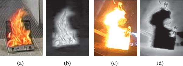
Two examples for the generalized mass transformation Eq. (9). (a) and (c): Original images. (b) and (d): Respective generalized mass (black - 0, white - 1). Fire texture is preserved, saturated regions are assigned as low mass.
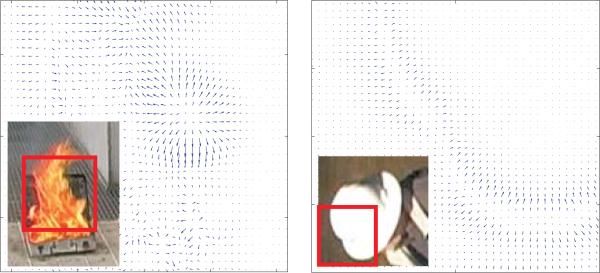
Note that fire classification is not performed based on the output of Eq. (9); this is a preprocessing step to obtain the image on which optical flow is computed. For this reason, the proposed color model does not have to be as accurate as when used as a feature. Fig. 5 shows two examples of OMT flow fields computed from the generalized mass images. It illustrates OMT's ability to capture dynamic texture for the fire image and discriminate between the rigid object's flow field, which appears much more structured.
Fig. 5.
OMT flow fields: fire with dynamic texture (left) and a white hat (right) moving up/right. The red box indicates the area for which the flow field is shown.
C. Non-Smooth Data (NSD) Optical Flow
Under unfavorable lighting conditions, especially in closed spaces, fire blobs are likely saturated, thus violating OMT's assumption that dynamic texture is present in fire. Nevertheless, these blobs have boundary motion, which may be characterized by another type of optical flow estimation. A novel optical flow energy functional called Non-Smooth Data optical flow (NSD) and tailored to saturated fire blobs is proposed as
| (11) |
The choice of the data term being the optical flow constraint Eq. (1) is justified because pixel saturation trivially implies intensity constancy. Also, the NSD is explicitly chosen to be non-smooth since saturated fire blobs are expected to have non-smooth boundary motion. The norm of the flow vector regularizes the flow magnitude, but does not enforce smoothness. This choice, therefore, makes the NSD flow directions purely driven by the data term under the constraint that flow magnitudes are not too large. While this method is not expected to perform well for standard optical flow applications where flow smoothness plays an important role, it proves useful for detecting saturated fire.
The solution to the minimization problem Eq. (11) is as simple as applying basic arithmetic operations to pre-computed image properties (as opposed to solving a system of equations), which means the NSD optical flow is computationally inexpensive. The Euler-Lagrange equations of Eq. (11) are written as
| (12a) |
| (12b) |
which, after a few manipulations, yield the solution
| (13) |
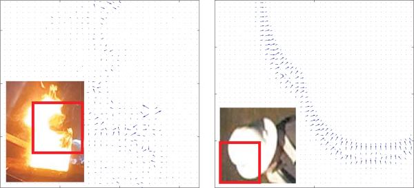
Again, Ix, Iy, and It are pre-computed image derivatives and α is the regularization parameter. Fig. 6 shows NSD flow fields computed for a saturated fire and a rigidly moving hat. Fire motion on the boundary is non-smooth in contrast to the hat's motion—a result from the data-driven formulation of the NSD.
Fig. 6.
NSD flow fields: saturated fire (left) and a white hat (right) moving up/right. The red box indicates the area for which the flow field is shown.
The following Section III illustrates characteristic fire features that are extracted from the flow fields derived above.
III. Optical Flow Features
A naive approach to vision-based detection is to use a supervised machine learning algorithm trained directly on intensity values in the image. This approach will undoubtedly underperform because the classification complexity increases exponentially with the dimensionality of the problem, which in this case is equal to the number of pixels. Further, the computational cost and the amount of training data required become prohibitively large. Instead, feature extraction is employed by incorporating prior information (known physical properties of the problem or human intuition) for the purpose of reducing the problem dimensionality.
The optical flow computations in Section II do not reduce dimensionality, as the two M × N images determine the values of the M · N, 2D, optical flow vectors. This transformation is an intermediate step that provides a data set from which motion features can be extracted more intuitively than would be possible from the original image. To do so, we pursue a region-based as opposed to a pixel-based approach. Whereas the pixel-wise approach classifies each pixel, the region-wise approach aims to classify a region as a whole by analyzing the set of all pixel values (in this case flow vectors) in that region. In the following section, the proposed feature extraction is defined and motivated.
A. Pre-Selection of Essential Pixels
Static or almost static image regions should be excluded from consideration because our aim is to characterize the type of motion an object is undergoing and they interfere with the motion statistics. For example, the average flow magnitude of a moving object should not depend on the size of the static background, which would be the case if the average was computed over the entire image instead of just the moving region. The set of essential pixels, which are pixels in motion, will therefore be defined as follows. Consider a frame or a subregion of that frame . (Working on subregions is imperative when there are several sources of motion in one frame, as explained in Section IV-A). Assume that the optical flow field is computed. Then, the set of essential pixels is defined as
| (14) |
where 0 ≤ c < 1 is chosen such that a sufficiently large number of pixels is retained. In case of extreme outliers, the parameter can be adjusted adaptively. For the data in Section V-A, a value of c = 0.2 provides sufficient motion segmentation across the database. In addition, reliability measures [13] could be employed to suppress pixels with low motion information. Some of the operations of feature extraction will be performed on this subset Ωe of “sufficiently moving” pixels.
B. Feature Extraction
In [13] a list of optical flow features is introduced, which is complete in that it considers all possible first-order distortions of a pixel. Those distortions are then averaged within a spatio-temporal block to yield the probability of a characteristic direction or of a characteristic magnitude. Reference [13] also mentions that the highest discriminating power comes from the characteristic direction and magnitude of the flow vector itself, not considering distortions. This observation matches our experience from early prototyping where flow derivatives seemed to have very little discriminating power and were thus removed from further consideration. Given the flow vectors, we propose four features i = 1, . . ., 4 defining the four dimensional feature vector F = (f1, f2, f3, f4)T. These features share the general idea with [13] to use “characteristic” motion magnitude and direction, yet are not the same. In particular, our magnitude features f1 and f2 measure mean magnitude as opposed to relative homogeneity of the magnitudes within a block in [13]. Our choice is straightforward for fire detection considering the color transformation in Section II-B2, thus biasing the detector to fire-like colored moving objects. The other two features f3 and f4 then analyze motion directionality. The OMT feature f3 takes into account spatial structure of the flow vectors, a strategy not considered in [13] where all vectors are averaged regardless of their location. Moreover, whereas [13] identifies the presence of one characteristic direction, feature f4 is more general in that it can detect multiple characteristic directions. Thus, given an image region and the optical flow fields and in that region, the features are chosen as follows.
1) OMT Transport Energy
This feature measures the mean OMT transport energy per pixel in a subregion
| (15) |
After the color transformation in Section II-B2, fire and other moving objects in the fire-colored spectrum, are expected to produce high values for this feature.
2) NSD Flow Magnitude
Similarly, the mean of the regularization term of the NSD optical flow energy Eq. (11) constitutes the second feature
| (16) |
The first two features, f1, f2, will have high values for moving, fire-colored objects. The last two features distinguish turbulent fire motion from rigid motion by comparing flow directionality.
3) OMT Sink/Source Matching
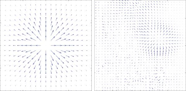
It is known [30] that solutions to OMT problems are curl-free mappings. For the turbulent motion of fire, this property tends to create flow fields with vector sinks and sources, a typical case of which is displayed in Fig. 7(b). For rigid motion, the flow field tends to be comprised of parallel vectors indicating rigid translation of mass.
Fig. 7.
(a) Ideal source flow template and (b) OMT flow field for the fire image in Fig. 5. The source matching feature is obtained by the maximum absolute value of the convolution between (a) and (b).
The third feature is designed to quantify how well an ideal source flow template matches the computed OMT flow field. The template is defined as
| (17) |
and shown in Fig. 7(a). Then, the best match is obtained by
| (18) |
where denotes convolution.
4) NSD Directional Variance
The final feature distinguishes the boundary motion of saturated fire blobs from rigidly moving objects by quantifying the variance of flow directions at moving pixels. A high variance suggests uncor-related motion in many different directions, whereas a low variance characterizes nearly uni-directional motion.
The implementation starts by estimating the flow field histogram
| (19) |
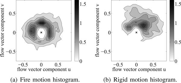
using kernel density estimation [31]. For notational convenience, the histogram h(r, ϕ) is written in polar coordinates, where represents the flow vector magnitude and ϕ = arctan (v/u) the flow vector direction. Fig. 8 shows the motion histograms of the flows from Fig. 6. As expected, the flow vectors for fire motion are scattered around the origin, whereas the flow vectors for rigid motion point predominantly in one direction (up and to the right, in this case). This correlation is measured by the fourth feature as
| (20) |
where
| (21) |
The domain is discretized into wedges si, and each si represents the ratio of pixels whose flow vector points in a direction between 2πi/n < ϕ ≤ 2π(i + 1)/n. For a flow field pointing mainly in one direction, only a few of the si are large, and consequently, the value for f4 is high. On the other hand, if the proportion of vectors pointing in each direction is approximately equal, all of the si will be similar, and f4 will have a low value.
Fig. 8.
Motion histograms for flows in Fig. 6. (a) (fire) has a multi-directional distribution, whereas (b) (hat) is dominantly moving up and right.
Feature f4 is more versatile for detecting rigid motion than the probability of a characteristic flow direction in [13]: For example, consider a flow field where half of the pixels point in one direction, and half in the opposite direction, which we would associate with rigid motion having two characteristic directions. Feature f4 will still yield a fairly high value indicating rigid motion, whereas in [13] the probability of a characteristic motion is practically zero since opposite vectors cancel each other out.
IV. Detection Algorithm
This section touches on two more topics required for an end-to-end detection system. Section IV-A shows how candidate regions, i.e., suspicious subregions of the image, can be created automatically and why this step is important. Then, Section IV-B explains how a candidate region is classified as fire or non-fire based on its feature vector, F.
A. Providing Candidate Regions
Computing optical flow and extracting features from an entire frame is unfavorable for two reasons. First, computation time increases as the domain Ω grows, and more importantly, the classification fails for scenes with more than one source of motion (e.g., a fire in the corner and a person walking in the center) since the motion statistics of the regions will be averaged and become no longer discriminatory. Therefore, it is essential for the proposed method that a segmentation of different sources of motion be provided, which the detection algorithm then classifies individually.
A connected region containing a single source of motion is called a candidate region. There may be more than one candidate region in the current image, , i = 1, 2,..., N and for each frame where N varies with time. Many publications construct candidate regions from color values and background estimation. Given a candidate region Ωc, optical flow is computed on Ωc, the features in Section III are computed, and Ωc is classified as a fire or nonfire region. While this approach is sufficient for our purposes, a more powerful method is given by tracking candidate regions using active contours as proposed by [32]. Briefly, a candidate region is defined by an active contour based on the Chan-Vese energy [33] that separates the mean of the optical flow magnitude inside and outside of the contour. The main advantage of tracking contours over time is that previous classification results of a candidate region can be incorporated in the current decision.
This paper focuses on optical flow features. Hence, it is assumed that homogeneous (i.e., belonging to the same moving object or part of the background) candidate regions are available.
B. Region Classification via Neural Network
The simplest way of classifying a candidate region based on its feature vector F = (f1, f2, f3, f4)T is to threshold each of the features fi based on heuristically determined cutoff values and make a decision by majority voting. However, better results can be achieved by learning the classification boundary with a machine learning approach such as neural networks. Training the neural network (NN) means performing a non-linear regression in the feature space to best separate the labeled training data into classes. Given a set of feature vectors F̄n, n = 1, . . ., N and their respective true class C̄n (e.g., C̄n = 1 (C̄n = 0) means contour n is a fire (non-fire) blob), the regression model used in a NN is
| (22) |
Here, the σ(·) is an activation function and the Φm(·) are fixed basis functions. The goal is to find the weights w = (w1, ..., wM) that minimize an error function
| (23) |
The basis functions used for this paper are
| (24) |
where features, fn, are the inputs to the NN and h(·) is an activation function (so-called hidden unit), typically taken be a sigmoid.
During the training phase, training examples are provided {F̄n, C̄n), n = 1,..., N} and the energy in Eq. (23) is optimized wm and wmn. In the testing phase, a feature vector F is supplied and the output in Eq. (22) is a probability that the feature vector F is associated with a particular class.
Note that neural networks are just one of many possible choices for learning the class separation boundaries. For instance, support vector machines (SVM) are expected to produce similar results. Selecting discriminatory features, not choosing the classifier, is most important for correct classification. More information on these topics can be found in [34].
V. Analysis and Test Results
The results section evaluates the proposed features’ performance in three ways. First, the algorithm is tested on a large video database. Since the absolute values of false detection rates are highly dependent on the testing and training data, a qualitative assessment of the results follows. Finally, a novel method of analyzing fire detectors is introduced by using synthetic fire simulations; they allow for a quantitative investigation into how flame saturation, spatial resolution, frame rate and noise influence detection.
A. Tests on Video Database
The algorithm is tested on a database provided by United Technologies Research Center (UTRC), Connecticut, USA. The database features various scenarios including indoor/outdoor, far/close distance, different types of flames (wood, gas, etc.), changing lighting conditions, partial occlusions, etc. The videos have a frame rate of 30 frames/second and spatial dimension of 240 by 360 pixels. From each of the 263 scenarios (containing 169 fire and 94 non-fire sequences), 10 consecutive frames are labeled as ground truth providing a test database of 2630 frames. Note that the non-fire scenarios are chosen to be probable false positives, namely moving and/or fire-colored objects such as cars, people, red leaves, lights and general background clutter. A neural network was trained on frames from 20 of those videos not used in the test database. The test result shows that fire is reliably detected using optical flow features only: the false positive rate (fire is detected when no fire is present) is fp = 3.19% and the false negative rate (no fire detected where there is a fire) is fn = 3.55%. These false detections rates are competitive with recently published, full-fledged fire detection systems, e.g. [2]: fp = 31.5%, fn 1.0%, [3]: fp 0.68%, fn 0.028%, [4]: fp = 0.30%, fn = 12.36% [12] (average among test videos): fp = 3.34%, fn = 21.50%. Since this paper explores the discriminatory power of optical flow features only rather than building a complete fire detector, we report the false detection rates as a feasibility check that the proposed features work on a large set of data. More careful analyses of the detector's properties and limitations, are explored in the following paragraphs.
B. Qualitative Analysis on Real Videos
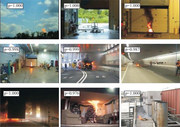
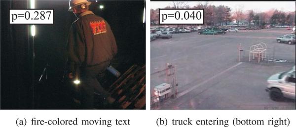
Example scenarios from the above tests are given in this section to illustrate successful classifications as well as typical false detections and their causes. Fig. 9 illustrates successful fire detections and Fig. 10 shows two examples of correctly classified non-fire scenes. In Fig. 10, the printing on the jacket and the truck entering at the bottom right are moving, fire-like colored (the truck has a reddish tint) objects. Nevertheless, due to their structured motion, these scenarios are correctly classified as not fire.
Fig. 9.
Examples of detected fire scenes with the resulting probabilities.
Fig. 10.
Examples of potential false positives correctly classified as non-fire scenes with the resulting probabilities.
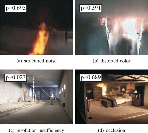
Occasional false negative detections were observed in four types of scenarios. First, horizontal lines resulting from structured noise in Fig. 11(a) introduce structure to the otherwise turbulent fire motion. Structured noise must to be avoided, therefore, when using the proposed features. Second, as in Fig. 11(b), the flame color is oddly distorted to a blue tinge which causes the color transformation in Eq. (9) to assign low mass and thus, low motion magnitude. Third, insufficient spatial resolution, as in Fig. 11(c), leads to very few pixels belonging to fire and motion structure cannot be detected. Lastly, partial occlusions may make the detector fail, as shown in Fig. 11(d), because the occluding object's edge causes motion vectors along that edge to be strongly aligned in the direction of the image gradient. Line detection algorithms could be employed as a preprocessing step to exclude edge pixels from consideration.
Fig. 11.
Examples of false negative detections (Fire scene falsely classified as non-fire scene) with the resulting probabilities.
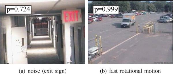
Regarding false positive detections, two deficiencies were observed. In Fig. 12(a), random noise on the red exit sign causes the motion field to have significant magnitude and turbulent directionality. Noise-reducing preprocessing can alleviate this problem, but other problems such as loss of texture detail may arise as a result. If spatial resolution is sufficient, multi-resolution techniques could be considered as well. Another false detection was observed for fast rotational motion (in combination with low spatial resolution) as seen in the case of the orange print on the truck in Fig. 12(b); the truck makes a sharp turn and undergoes a large perspective change. A change in perspective does not satisfy the intensity constancy assumption Eq. (1) as self-occlusions occur and intensity disappears during the rotation. In order to successfully reject such scenarios, a track-and-detect algorithm as proposed in [32] can monitor the scene and set off alarm only if the anomaly persists.
Fig. 12.
Examples of false positive detections (Non-fire scene falsely classified as fire scene) with the resulting probabilities.
C. Quantitative Analysis on Simulated Videos
Lastly, an experiment is presented that further illustrates and substantiates the key idea of the paper. Since this experiment is based on synthetic data from fire simulations, there is a controlled test environment that allows for the quantitative analysis of parameter influences such as flame saturation, spatial resolution, frame rate and random noise. The fire simulator and relevant files can be downloaded at https://github.com/pkarasev3/phosphorik.
Fire Simulation
Fire simulation has become an important tool in modern multi-media applications such as movies, video games, etc. In our application, these simulations serve to generate synthetic ground truth for testing of the vision-based fire detector. Clearly, the physics of fire cannot be modeled exactly, but the basic physical laws are well explored in the field of continuum mechanics [35]. Furthermore, despite not mimicking real fire videos precisely, simulations pose similar challenges for a fire detector but in a way that can be quantified. The fire simulations used in this paper are inspired by [36], [37] and employ the inviscid Euler equations [27] to model the physics. From the simulated physical quantities such as heat and pressure, images are rendered using concepts such as light scattering and color models.
Experiment
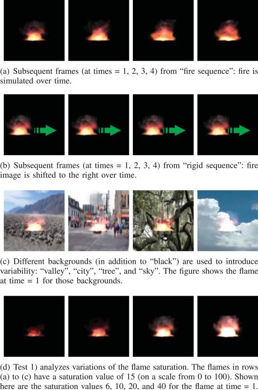
We create a sequence of images where fire is simulated (fire sequence), as shown in Fig. 13(a). We then create another sequence of images made up of identical fire frames shifted horizontally left to right (rigid sequence). The size of the shift is chosen such that the energy features f1 and f2 in Eq. (15) and (16) are similar to the ones in the fire sequence. Frames from the rigid sequence are shown in Fig. 13(b). The same process is repeated for four more backgrounds other than black, as shown in Fig. 13(c). Note that the background affects the rendering of the fire flame; so, different backgrounds introduce some variability in the appearance of the flame. Overall, there are five fire and five rigid sequences. The goal is to distinguish between a fire and a moving image of a fire in a video based on the directional features f3 and f4 in Eq. (18) and (20). We observe that just about any static feature used in the literature will typically fail this experiment, as will many temporal features if they only quantify the magnitude of the change.
Fig. 13.
Sample frames from the fire simulation experiment.
Analysis
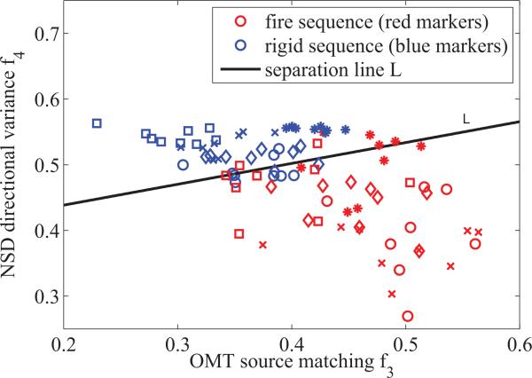
Fig. 14 plots the feature values f3 and f4 for the frames of the experiment described above. Intuitively, if the data points from the rigid sequences are well separated from the points belonging to the fire sequences, the features effectively discriminate between the two classes (rigid and fire). How well the features discriminate will be measured quantitatively by fitting a line L in the f3–f4 space such that the two classes are best separated i.e,
| (25) |
is minimized. Here, is the feature point for frame i in the f3- f4 space. The weighting function w(i) is defined as
| (26) |
and assures that points on the wrong side of L are penalized more to achieve the best possible separation. The optimal separation line L is also plotted in Fig. 14. As expected, the directional features are capable of separating the feature points with only a few points lying on the wrong side, but still close to the separation line.
Fig. 14.
Directional features f3 and f4 for frames from the simulation experiment. Each marker corresponds to one frame. Different markers indicate different backgrounds: asterisk - black, circle - city, cross - tree, diamond -valley, and square - sky. The separation line L best separates the two clusters according to Eq. (25).
The resulting minimal error Emin for Eq. (25) quantifies how well the directional features perform in the experiment. Moreover, the slope s of L indicates which feature is having a bigger impact; for instance, if the slope is large, the OMT feature f3 explains the difference between classes to a large degree, and if the slope is small, the NSD feature f4 is most discriminatory. Based on these two quantities, the following experiments analyze the influence of video parameter changes.
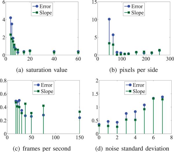
1) Flame Saturation
The first experiment was performed using a flame saturation value of 15. In the fire simulations, it is possible to vary the saturation value that changes flames from totally transparent (value 0) to totally white or fully saturated (value 100). Frames for several different saturation values are shown in Fig. 13(d). Repeating the above experiment for different saturation values, the analysis of the result in terms of Emin and the slope of the separation line s, yields Fig. 15(a). It is observed that the error first decreases for increasing saturation and then increases for saturations of higher than 10. This result shows that the detector performs best when the flame is not too dim and not too saturated. Moreover the slope s tends to decrease with higher saturation, which is expected since the OMT feature f3 was designed for dynamic textures, and the NSD feature f4 dominates when the flame is saturated and appears more like a rigid object.
Fig. 15.
Influence of parameter changes on the error Eq. (25) and the slope of the separation line L in Fig. 14.
2) Spatial Resolution
In this experiment, we vary the size of the images. The images shown so far have been 128 × 128 pixels. By repeating the experiments for different image sizes with the flame size changing proportionally, Fig. 15(b) is obtained. The key observation is that there is a certain minimum size of about 70 × 70 pixels needed to guarantee sufficient resolution to compute apparent motion. Above this minimum size, performance is almost invariant under spatial resolution. The slope of the separation line (apart from the first two stems where the detector breaks) seems positively related to the image size, i.e. the OMT feature relies more on a high spatial resolution than the NSD feature does.
3) Frame Rate
It is known that fire flickers at a rate of roughly 10 H z. To relate simulation time to real time, the flicker rate in the simulation is compared to this rate. Thus, the time step in the simulation can be chosen to correspond to a particular frame rate in real time. A slightly decreasing trend is observed for the error in Fig. 15(c), when increasing the frame rate from initially 30 frames/sec. The absolute change is small compared to the size changes seen above; this means that the features are robust with respect to temporal resolution. No correlation between the slope of the separation line and the frame rate is observed.
4) Gaussian Noise
Finally, the influence of random noise is studied. Each channel of the RGB-images (scaled between 0 and 255) is perturbed by additive, zero mean, i.i.d. Gaussian noise while the standard deviation is varied. As seen in Fig. 15(c), up to a standard deviation of 7, the detector is separating the two types of motion increasingly worse. For standard deviations higher than 7, the detector can no longer discriminate between classes. Random noise should, therefore, be avoided when applying the proposed features. The slope is increasing with the noise level as well; this occurs because the NSD optical flow is error-prone to local noise. The OMT optical flow, on the other hand, connects neighboring pixels in its system matrix, thus allowing for some smoothing effect to take place.
D. Comparison to OpenCV Horn-Schunck
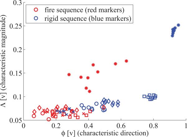
This last section intends to show the inadequacy of standard Horn-Schunck for fire videos, a claim made earlier in the paper. For that purpose, the simulation experiment from Section V-C resulting in Fig. 14 is repeated for the OpenCV implementation of Horn-Schunck (CVHS), which is shown to work best among the methods considered in [13] for dynamic texture recognition. In our tests, different choices for the regularization parameter (λ = 0.25 and λ = 0.5) do not result in qualitative differences. In order to be able to compare the experiment to Fig. 14, the best two features from [13] are extracted from the CVHS flow fields, which are the probability of having a characteristic direction ϕ[v] and of having a characteristic magnitude Λ[v]. Fig. 16 shows the result for the simulated fire (red) and the rigidsequence (blue).Whereas the CVHS features work well for a black background, scene variability in form of non-trivial backgrounds make the features unreliable: The feature points in the bottom-left corner strongly overlap for fire and rigid scenes. Moreover, observe that for the rigid sequences, the CVHS features form separated clusters for each background, whereas for the fire sequences, the features are all mixed (except for black background). This shows that standard Horn-Schunck yields consistent results for different backgrounds in the case of rigid motion, but becomes unpredictable for fire content since fire does not satisfy the brightness constancy plus smoothness assumptions.
Fig. 16.
From OpenCV Horn-Schunck (CVHS) computed on the simulation experiment in Section V-C, the probability of characteristic direction ϕ[v] and the probability of characteristic magnitude Λ[v] as defined in [13] are extracted. This figure stands in direct comparison to Fig. 14 (asterisk - black, circle - city, cross - tree, diamond - valley, square - sky). It is observed that CVHS works well only for black background, whereas for non-trivial backgrounds, the features become unreliable.
VI. Conclusion
The very interesting dynamics of flames have motivated the use of motion estimators to distinguish fire from other types of motion. Two novel optical flow estimators, OMT and NSD, have been presented that overcome insufficiencies of classical optical flow models when applied to fire content. The obtained motion fields provide useful space on which to define motion features. These features reliably detect fire and reject non-fire motion, as demonstrated on a large dataset of real videos. Few false detections are observed in the presence of significant noise, partial occlusions, and rapid angle change. In an experiment using fire simulations, the discriminatory power of the selected features is demonstrated to separate fire motion from rigid motion. The controlled nature of this experiment allows for the quantitative evaluation of parameter changes. Key results are the need for a minimum spatial resolution, robustness to changes in the frame rate, and maximum allowable bounds on the additive noise level. Future work includes the development of optical flow estimators with improved robustness to noise that take into account more than two frames at a time.
Acknowledgments
This work was supported by the Office of Naval Research under Contract N00014-10-C-0204, Grants from AFOSR and ARO, Grants from the National Center for Research Resources under Grant P41-RR-013218, the National Institute of Biomedical Imaging and Bioengineering under Grant P41-EB-015902 of the National Institutes of Health, and the National Alliance for Medical Image Computing, funded by the National Institutes of Health through the NIH Roadmap for Medical Research, under Grant U54 EB005149. The associate editor coordinating the review of this manuscript and approving it for publication was Prof. Hassan Foroosh.
Biography
 Martin Mueller received the M.S. degree in civil and environmental engineering from the Georgia Institute of Technology, Atlanta, GA, USA, in 2009, and the Diplom-Ingenieur degree in engineering cybernetics from the University of Stuttgart, Stuttgart, Germany, in 2010. He is with the School of Electrical and Computer Engineering with Georgia Tech.
 Peter Karasev received the B.S., M.S., and Ph.D. degrees in electrical and computer engineering from Georgia Tech, Atlanta, GA, USA, in 2008, 2010, and 2013, respectively. He is a Research Engineer with the Department of Electrical and Computer Engineering at the University of Alabama at Birmingham, Birmingham, AL, USA. His current research interests include the application of control-theoretic methods to medical image processing and computer vision.
 Ivan Kolesov received the Ph.D. degree in electrical and computer engineering from the Georgia Institute of Technology, Atlanta, GA, USA, in 2012. He is currently a Postdoctoral Researcher with the Department of Electrical and Computer Engineering at the University of Alabama at Birmingham, Birmingham, AL, USA. His current research interests include the fields of computer vision and machine learning.
 Allen Tannenbaum received the Ph.D. degree in mathematics from Harvard University, Cambridge, MA, USA, in 1976. He is with the Department of Electrical and Computer Engineering, the University of Alabama at Birmingham, Birmingham, AL, USA, and the Comprehensive Cancer Center, UAB.
Footnotes
The videos were provided by courtesy of United Technologies Research Center, Connecticut, USA.
Contributor Information
Martin Mueller, Department of Electrical and Computer Engineering, Georgia Institute of Technology, Atlanta, GA 30332 USA (martin.mueller@gatech.edu)..
Peter Karasev, Department of Electrical and Computer Engineering, University of Alabama at Birmingham, Birmingham, AL 35294 USA (pkarasev@gatech.edu)..
Ivan Kolesov, Department of Electrical and Computer Engineering, University of Alabama at Birmingham, Birmingham, AL 35294 USA (ivan.kolesov1@gmail.com)..
Allen Tannenbaum, Comprehensive Cancer Center and Department of Electrical & Computer Engineering, University of Alabama at Birmingham, Birmingham AL 35294 USA (tannenba@uab.edu)..
REFERENCES
- 1.du Bartas G. La Sepmaine ou Creation du Monde. Michel Gadoulleau et Jean Febvrier; Paris, France: 1578. [Google Scholar]
- 2.Çelik T, Demirel H. Fire detection in video sequences using a generic color model. Fire Safety J. 2009;44(2):147–158. [Google Scholar]
- 3.Borges P, Izquierdo E. A probabilistic approach for vision-based fire detection in videos. IEEE Trans. Circuits Syst. Video Technol. 2010 May;20(5):721–731. [Google Scholar]
- 4.Ho C. Machine vision-based real-time early flame and smoke detection. Meas. Sci. Technol. 2009;20(4):045502. [Google Scholar]
- 5.Marbach G, Loepfe M, Brupbacher T. An image processing technique for fire detection in video images. Fire Safety J. 2006;41(4):285–289. [Google Scholar]
- 6.Liu C, Ahuja N. Vision based fire detection. Proc. Int. Conf. Pattern Recognit. 2004;4:134–137. [Google Scholar]
- 7.Zhao J, Zhang Z, Han S, Qu C, Yuan Z, Zhang D. SVM based forest fire detection using static and dynamic features. Comput. Sci. Inf. Syst. 2011;8(3):821–841. [Google Scholar]
- 8.Toreyin B, Dedeoglu Y, Gudukbay U, Cetin A. Computer vision based method for real-time fire and flame detection. Pattern Recognit. Lett. 2006;27(1):49–58. [Google Scholar]
- 9.Ko B, Cheong K, Nam J. Fire detection based on vision sensor and support vector machines. Fire Safety J. 2009;44(3):322–329. [Google Scholar]
- 10.Verstockt S, Vanoosthuyse A, Van Hoecke S, Lambert P, Van de Walle R. Multi-sensor fire detection by fusing visual and non-visual flame features. Proc. 4th Int. Conf. Image Signal Process. 2010:333–341. [Google Scholar]
- 11.Phillips W, III, Shah M, da Vitoria Lobo N. Flame recognition in video. Pattern Recognit. Lett. 2002;23(1–3):319–327. [Google Scholar]
- 12.Habiboglu Y, Günay ȈO, Çetin A. Covariance matrix-based fire and flame detection method in video. Mach. Vis. Appl. 2011;23(6):1–11. [Google Scholar]
- 13.Fazekas S, Chetverikov D. Analysis and performance evaluation of optical flow features for dynamic texture recognition. Signal Process., Image Commun. 2007;22(7–8):680–691. [Google Scholar]
- 14.Chetverikov D, Péteri R. A brief survey of dynamic texture description and recognition. Proc. Int. Conf. Comput. Recognit. Syst. 2005:17–26. [Google Scholar]
- 15.Fazekas S, Amiaz T, Chetverikov D, Kiryati N. Dynamic texture detection based on motion analysis. Int. J. Comput. Vis. 2009;82(1):48–63. [Google Scholar]
- 16.Chetverikov D, Fazekas S, Haindl M. Dynamic texture as foreground and background. Mach. Vis. Appl. 2011;22(5):741–750. [Google Scholar]
- 17.Chunyu Y, Jun F, Jinjun W, Yongming Z. Video fire smoke detection using motion and color features. Fire Technol. 2010;46(3):651–663. [Google Scholar]
- 18.Lucas B, Kanade T. An iterative image registration technique with an application to stereo vision. Proc. Int. Joint Conf. Artif. Intell. 1981;2:674–679. [Google Scholar]
- 19.Saisan P, Doretto G, Wu Y, Soatto S. Dynamic texture recognition. Proc. Conf. Comput. Vis. Pattern Recognit. 2001;2:58–63. [Google Scholar]
- 20.Doretto G, Chiuso A, Wu Y, Soatto S. Dynamic textures. Int. J. Comput. Vis. 2003;51(2):91–109. [Google Scholar]
- 21.Cooper L, Liu J, Huang K. Spatial segmentation of temporal texture using mixture linear models. Proc. Int. Conf. Dyn. Vis. 2007:142–150. [Google Scholar]
- 22.Chan A, Vasconcelos N. Modeling, clustering, and segmenting video with mixtures of dynamic textures. IEEE Trans. Pattern Anal. Mach. Intell. 2008 May;30(5):909–926. doi: 10.1109/TPAMI.2007.70738. [DOI] [PubMed] [Google Scholar]
- 23.Vidal R, Ravichandran A. Optical flow estimation & segmentation of multiple moving dynamic textures. Proc. IEEE Comput. Soc. Conf. Comput. Vis. Pattern Recognit. 2005 Jun;2:516–521. [Google Scholar]
- 24.Kolesov I, Karasev P, Tannenbaum A, Haber E. Fire and smoke detection in video with optimal mass transport based optical flow and neural networks. Proc. IEEE Int. Conf. Image Process. 2010 Sep;:761–764. [Google Scholar]
- 25.Horn B, Schunck B. Determining optical flow. Artif. Intell. 1981;17(1–3):185–203. [Google Scholar]
- 26.Baker S, Scharstein D, Lewis J, Roth S, Black M, Szeliski R. A database and evaluation methodology for optical flow. Int. J. Comput. Vis. 2007;92(1):1–31. [Google Scholar]
- 27.Malvern L. Introduction to the Mechanics of a Continuous Medium. Prentice-Hall; Upper Saddle River, NJ, USA: 1969. [Google Scholar]
- 28.Benamou J, Brenier Y. A computational fluid mechanics solution to the Monge-Kantorovich mass transfer problem. Numer. Math. 2000;84(3):375–393. [Google Scholar]
- 29.Kantorovich L. On the translocation of masses. J. Math. Sci. 2006;133(4):1381–1382. [Google Scholar]
- 30.Gangbo W, McCann R. The geometry of optimal transportation. Acta Math. 1996;177(2):113–161. [Google Scholar]
- 31.Botev Z, Grotowski J, Kroese D. Kernel density estimation via diffusion. Ann. Stat. 2010;38(5):2916–2957. [Google Scholar]
- 32.Mueller M, Karasev P, Kolesov I, Tannenbaum A. A video analytics framework for amorphous and unstructured anomaly detection. Proc. 18th IEEE Int. Conf. Image Process. 2011 Sep;:2945–2948. [Google Scholar]
- 33.Chan T, Vese L. Active contours without edges. IEEE Trans. Image Process. 2001 Feb;10(2):266–277. doi: 10.1109/83.902291. [DOI] [PubMed] [Google Scholar]
- 34.Bishop C. Pattern Recognition and Machine Learning (Information Science and Statistics) Springer-Verlag; New York, NY, USA: 2006. [Google Scholar]
- 35.Quintiere J. Fundamentals of Fire Phenomena. Wiley; New York, NY, USA: 2006. [Google Scholar]
- 36.Nguyen D, Fedkiw R, Jensen H. Physically based modeling and animation of fire. ACM Trans. Graph. 2002;21(3):721–728. [Google Scholar]
- 37.Fedkiw R, Stam J, Jensen H. Visual simulation of smoke. Proc. Conf. Comput. Graph. Interact. Tech. 2001:15–22. [Google Scholar]


