General Principles for Measuring Resting Membrane Potential and Ion Concentration Using Fluorescent Bioelectricity Reporters

Abstract

This overview provides the basic information needed to understand, choose, and use fluorescent bioelectricity reporters (FBRs), where bioelectricity is defined as cell processes that involve ions or ion flux. While traditional methods of measuring these characteristics are still valid and necessary, the utility of FBRs has facilitated measurement of these properties under circumstances that are not possible with microelectrodes. Specifically, these dyes can be used to achieve subcellular resolution, to measure many cells simultaneously in vivo, and to track bioelectric gradients over long time periods despite cell movements and divisions. This article covers the basic principles underlying the interpretation of the dye signals, describes essential steps for troubleshooting, optimizing data collection, analysis, and presentation, and provides compilations of information that are useful for choosing FBRs for particular projects.

INTRODUCTION

Electrophysiology, defined here as the study of ion and ion-flux dependent cellular phenomena, yields information about a fundamental aspect of biology: all cells regulate ion concentrations and maintain electric potentials across their membranes. It is widely accepted that the functions of the brain, heart, and skeletal muscle depend on bioelectrical signals in the form of action potentials. Likewise, the roles of ion gradients in chloroplasts and mitochondria are well-known. However, changes in resting transmembrane potential and individual ion flows are essential activities of all cells. It is now known that such bioelectrical signals, occurring on a scale of minutes to days, mediate crucial instructive signals that regulate cell behavior in vivo. The gating of ion channels and pumps produces transmembrane voltage gradients that control tissue patterning and axial polarity, and serve as an important component of the systems of cell:cell communication that integrate individual cellular activities into large-scale growth and form. Recent development of molecular genetic methods for the functional investigation of these signals and their linkage to known biochemical and genetic pathways have revealed a plethora of exciting new roles for such bioelectric signals in development, regeneration, and cancer (reviewed in Levin [2007]; Adams [2008]; Blackiston et al. [2009]; Levin [2009]; Sundelacruz et al. [2009]; Levin [2011])). An important component to all such investigations is the ability to track spatio-temporal distribution of membrane voltage (V_mem) gradients in vivo, over significant periods of time, without perforating the cell membrane.

Electrophysiological characteristics of cells can be measured using microelectrodes. These extremely fine glass needles can be used to impale cells, patch clamp, or measure ion concentrations. These techniques are extremely powerful for single cell measurements, and the quantitative data they produce remains the standard. The necessarily small size of a microelectrode, however, constrains the types of measurements possible, and the sample under study must be kept perfectly still.

More recently, the use of FBR of V_mem and ion concentration ([I]) has increased as continuing research and innovation have produced better and more options. These dyes are now used routinely for cell sorting and for studies of cultured cells. Important advantages offered by dyes are (1) subcellular resolution, (2) the ability to monitor multicellular areas and volumes, (3) simplicity of use, (4) ability to measure moving targets, and (5) ability to measure over long periods. This article will introduce the basic concepts and practical information needed to use these dyes, especially as concerns their use for physiology and developmental biophysics in vivo. It is assumed that the reader is fully familiar with the process and terminology of fluorescence microscopy. A protocol is also available for Measuring Resting Membrane Potential Using the Fluorescent Voltage Reporters DiBAC₄(3) and CC2-DMPE<prot067702> (Adams and Levin 2012).

Basic Categories of FBR

The fluorescent V_mem indicators (Table 1) come in two categories, based on the speed with which they can respond to a change in membrane potential. The slow-response probes include: the carbocyanine dyes (DiOs, DiIs, and JC-1 and -9); rhodamine in various forms; the oxonols (including Oxonol V and VI, DiBAC₄[3], DiBAC₄[5], and DiSBAC₂[3]); and Merocyanine 540. These dyes respond to changes by physically moving either in and out of a cell or between the two leaflets of a lipid bilayer (Fig. 1). One strategy for these dyes is to use them in combination with another fluorescent dye such that the fluorescence intensity of one can be normalized to the fluorescence intensity of the other and thereby factor out uneven illumination and other systematic error. This can be accomplished by pairing a cationic dye with an anionic dye (Fig. 2). In addition to providing the control for illumination (assuming that the two dyes are taken up equally, which condition may not be met; see controls), the intensity of the two dyes should go in opposite directions, a positive control that shows whether the intensity is changing due to V_mem changes or just artifactual redistribution of one or both dyes. Another kind of pairing exploits fluorescence resonance energy transfer (FRET) between the two dyes, where one of the dyes moves in response to V_mem changes (Fig. 3). Two such pairs combine CC2-DMPE, an oxycoumarin derivative that is restricted to the outer leaflet of the plasma membrane, with a mobile oxonol. These report V_mem changes as changes in FRET between the donor CC2-DMPE, which is immobilized in one leaflet of the membrane, and the oxonol which moves closer to or further away from the donor in proportion to V_mem. The FRET signal can then be normalized to the CC2-DMPE emission.

Table 1.

Fluorescent V_mem reporters and FRET-based V_mem reporters

FLUORESCENT VMEM REPORTERS
FBR (variants omitted unless λex differs)	Charge	Fast/Slow	λex	λem	Notes (see explanations below)
Aminonaphthylethenylpyridinium (ANEPX)	+/−	F	496	705	a
Di-3-ANEPPDHQ	+	F	512	712	a
Di-4-ANEPPS	+/−	F	468	635	a
Di-8-ANEPPS	+/−	F	440/500	631	e
DiBAC4(5)	−	S	590	616	a,(f)
DiBAC4(X)	−	S	493	516	a,f
DiIC1(5)	+	S	638	658	c
DiOCx(3)	+	S	482	497	c
DiSBAC2(X)	−	S	535	560	a,(f)
DiSC3(5)	+	S	651	675
HLB021-152			531	551
JC-1	+	S	514	529/570	c,e
Merocyanine 540		F/S	555	578	b,d
Oxonol V	−	S	610	639	a,(f)
Oxonol VI	−	S	599	634	a,(f)
RH 155	+	S	650		a
Rhodamine 123	+	S	507	529	c
Rhodamine 6G	+	S	525	555
TMRE	+	S	549	574	c

FRET-BASED VMEM REPORTERS	Donor λex	Donor λem	Acceptor λex	Acceptor λem
CC2-DMPE	425	435
EGFP-F	488	508
ECFP-F	434	477
PTSx	404	434
DACCA	410	460
DiBAC4(3)			497	517
DiSBAC2(3)			543	570
Mermaid	483	499	551	563

^a:Potentiates GABA_A receptors (Mennerick et al.2010)

^b:Phototoxic (Anaspec.com)

^c:Used for staining mitochondrial membranes

^d:Biphasic F/S response

^e:Ratiometric

^f:Activates large-conductance Ca²⁺-activated K⁺ channels (Morimoto et al. 2007)

^(f):f may apply because of molecular similarity, but hasn't been tested

^X:Position of differences in variants

Figure 1.

Basic mechanism of mobile cationic and anionic FBRs of V_mem. Intensity of the signal is proportional to the number of molecules of reporter in the membrane. The molecules are free to move in and out of the cell; outside the cell they are not fluorescent. If the inner leaflet of the membrane is negatively charged, anionic dyes exit the cell while cationic dyes enter, leading to the opposite change in fluorescence intensity.

Figure 2.

Pairing two dyes of opposite charge. If two dyes are used, the signals from the two can be compared or combined to give greater accuracy.

Figure 3.

FRET-based detection of V_mem. By combining two fluorophores that are a FRET pair, this approach ensures that the signals collected are being emitted from the same membrane.

The fast-response probes respond to changes in V_mem by undergoing a conformational change, which can happen much faster than the physical movement of slow-response probes. These are styryls (the ANEP dyes) and the RH dyes. Molecular genetics has been used to create fast-response V_mem reporters based on fluorescent proteins. Mermaid, for example, changes conformation in response to a change of V_mem, thus bringing together or separating a FRET donor and acceptor (Tsutsui et al. 2008). The strategy of combining an immobile FRET donor with a mobile acceptor that moves in response to V_mem changes is also the basis of certain fast reporters, such as EGFP (enhanced green fluorescent protein)-F and ECFP (enhanced cyan fluorescent protein)-F, which can then be paired with DiBAC₄(5), or dipicrylamine (DPA), a non-fluorescent acceptor (DiFranco et al. 2007). The fast-response probes are best suited for measuring action potentials, however. Thus, FBR characteristics that are important for studying resting potential or long-term changes, such as toxicity, tendency to bleach, or cell-type specific variations in accumulation, have not been characterized.

The fluorescent indicators of ion concentration (Table 2) are, in the best cases, simpler to use than the V_mem dyes. That is because many of them are ratiometric - they can emit both an ion-concentration sensitive signal and an ion-concentration insensitive signal resulting from illumination or emission at one particular wavelength (the isosbestic point and the isoemissive point respectively; Fig. 4). The image collected at the isosbestic or isoemissive wavelength is a perfectly-paired control: it is the same as the signal at the sensitive wavelength in all ways except the variable of interest, ion concentration. So, normalizing the sensitive signal to the insensitive signal (dividing the former by the latter) removes most of the artifacts that would otherwise contaminate the signal (Fig. 5 and Fig. 6). Specifically, it corrects for (1) variation in dye permeability and therefore dye concentration, and (2) uneven illumination and other systematic error in the system.

Table 2.

Fluorescent ion concentration reporters

Ion	Reporter (variants not included unless λex or kd differs)	λex 1	λex 2	λem 1	λem 2	kd[nM, unless otherwise indicated]
Ca2+	Quin	339	380	492		100
Ca2+	Fura	340	380	512		146
Ca2+	Indo	347		475	420
Ca2+	Fura red	425	500	637
Ca2+	Fluo	506		526		390
Ca2+	Rhod	549		578		570
Ca2+	Rhod-5F, tripotassium salt	551		577
Ca2+	Rhod-5F	580		602
Ca2+	X-Rhod	580		602		700
Cl−	Methoxy N ethylquinolinium iodide (MEQ)	344		442
Cl−	N Ethoxycarbonylmethyl methoxyquinolinium bromide (MQAE)	350		460
Cl−	Lucigenin	455		505
Cl−	Methoxy N sulfopropyl quinolinium (SPQ)	348		443
H+	HPTS	390	460	510
H+	Biscarboxyethylcarboxyfluorescein (BCECF)	503	439	528		pKa = 7.0
H+	Hydroxypyrene trisulfonic acid trisodium salt	454		511
H+	Fluorescein	490		514
H+	Oregon Green 488	490	440	514		pKa = 4.8
H+	Carboxyfluorescein diacetate (CFDA)	492	450	517		pKa = 6.5
H+	Carboxy-dichlorofluorescein (CDCF)	495	504	529		pKa = 4.8
H+	SNAFL-1	500		575	640	pKa = 7.8
H+	SNARF-1	500		575	631	pKa = 7.5
H+	Carboxy-Napthofluorescein	598	589	668	572	pKa = 7.6
H+	Oregon Green 514	510	450	529		pKa = 4.8
H+	SNARF-4F	520		592	661	pKa = 6.4
H+	X-NERP	520	570	610
H+	SNARF-5F	560		575	628	pKa = 7.2
H+	6-Joe	525		555
Ion2+ and La3+	Calcein	494	517
Ion2+ and La3+	Rhod-2 tripotassium salt	549		578
K+	PBFI	340	390	510
K+	Asante potassium green (APG)-x	500		540
Mg2+	Indo-1 Mg	343		417	480	2.7 mM
Mg2+	Fura-2 Mg	360	369	490		1.9 mM
Mg2+	Fluo-2 Mg	505		525		5.1 mM
Mg2+	Asante calcium X Mg	505		525		5.1 mM
Na+	SBFI	340	380	505		4 mM
Na+	Asante natrium green (ANG)-1	500		540		92 mM
Na+	Asante natrium green (ANG)-2	500		540		20 mM
Zn2+	Methoxy quinolyl toluenesulfonamide (TSQ)	344		385
Zn2+	Zinquin	360		500
Zn2+	TFL-Zn	360		498

Figure 4.

Spectra of dual emission pH reporter dye. This is an example of a dual-emission ratiometric ion reporter. When illuminated at λ_ex = 488 nm, signal collected at emission wavelength (λ_em) = 640 nm does not change with pH; the intensity of the signal collected at the maximum λ_em = 610 nm does change depending on the proportion of dye molecules that are protonated; thus, in proportion to the pH. The signal collected at the isoemissive wavelength (640 nm) is thus an image of all variation that is due to noise or error in the system, including the important variable of differential uptake of dye. By normalizing the signal at 610 nm to the signal at 640 nm, much of the error is removed.

Figure 5.

Dual excitation FBR for measuring ion concentration. The basic mechanism of dual excitation dyes is illustrated. The isosbestic point is the λ_ex at which the signal at λ_em is insensitive to changes in ion concentration. In this example, λ_ex of the bound reporter is lower than λ_ex of the unbound reporter. If the opposite were the case, the standard curve would have a positive slope.

Figure 6.

Dual-emission FBR for measuring ion concentration. The basic mechanism of dual emission dyes is illustrated. The isoemissive point is the λ_em at which the signal is insensitive to changes in ion concentration. In this example, λ_ex of the bound reporter is higher than λ_ex of the unbound reporter. If the opposite were the case, the standard curve would have a negative slope.

GENERAL PROTOCOLS FOR USING FBRs

To understand the guidelines for choosing and using (and troubleshooting) FBRs, it helps to be well-acquainted with the inherent difficulties; therefore, this section will begin with the bad news.

Difficulties and How to Deal with Them

You are not measuring V_mem/[I] (membrane voltage and/or ion concentration) - you are measuring the number of photons emitted from the sample that reached your computer as electrons. The first assumption is that the number of electrons is directly correlated with the number of fluorophores present; the second assumption is that the number is a simple function of the V_mem/[I] of interest. Artifacts arise because both assumptions can be violated.

Violations of the First Assumption

Electronic noise and other unavoidable imperfections in the equipment add error. If the signal is low, shot noise in particular can add significant uncertainty to the value of pixel intensity. The solution is to perform darkfield (DF) and flatfield (FF) correction (see Imaging below). These absolutely required corrections to the raw images involve image arithmetic (meaning the pixels in corresponding locations on two images are added, subtracted, etc.); specifically, dividing the raw image by a control image (also referred to as normalizing). Error is significantly reduced by propagation through the process of division.

Fluorescent dyes can bleach. As a direct result of being illuminated at the excitation wavelength (λ_ex), the dye loses the electrons it needs to be in an excited state, so there is no more returning to the unexcited state, hence no fluorescence emission. One solution is to perform control 5 below, to determine if this is a problem. If yes, focus on your region of interest using a different, preferably longer wavelength. The first exposure of the region to the λ_ex should be the one collected. Keep this constant throughout all the imaging (the FF image as well). A better solution is to use one of the dyes that does not bleach. This characteristic will be proudly advertised.

Fluorescent dyes can self-quench. Quenching is any process that reduces the emission of a fluorescent dye. If the concentration of the dye is too high, the molecules can over-excite and quench each other. Control 5 below can reveal this problem: as some of the dye is bleached, it will stop quenching, and fluorescence can increase. In any case, titer your dye concentration in both directions, starting at the published concentration, then use a concentration that responds appropriately in the range of V_mem values expected (control 1 below).

Violations of the Second Assumption

Many V_mem dyes are indiscriminate about which or how many membranes they will cross, and all internal membranes have voltages across them. Some V_mem dyes are known, for example, to accumulate in mitochondria (Table 1). The solution is to use sufficient subcellular resolution to identify which membranes are emitting signal. If that is not possible, be sure to state clearly in your results section that you do not know which membranes are involved. Indeed, the standing voltage gradients of intracellular compartments (such as nuclear envelope potential) have only just begun to be explored for instructive roles in control of cell behavior (Mazzanti et al. 2001; Tyner et al. 2007).

Some [I] FBRs are promiscuous about the ions they will bind (Table 2). To be sure that the concentration of other, similar ions is not confounding your measures, measure in the presence of ionophores that are specific for those other ions; if your dye is specific, there should be no effect on the measure. You may also be able to find a suitable dye that has been tested in this regard.

Different cells may be differently permeable to dyes; thus, differences in fluorescence may have nothing to do with V_mem/[I]. One solution is to use ratiometric techniques whenever possible. If there is no ratiometric dye available, repeat the experiment with as many dyes as possible to see whether the results are consistent.

Selecting an FBR

Figures 1–6 illustrate the mechanisms that FBRs employ. Each has advantages and disadvantages depending on the system under study. Many of the dyes have been used only in cultured cells or fluorescence-activated cell sorting (FACS); thus, complications arising from the study of in vivo processes, such as sample dimensions, opacity, autofluorescence, and movement have not been addressed. The power of these dyes to reveal bioelectrical mechanisms (Beane et al. 2011; Blackiston et al. 2011; Vandenberg et al. 2011b),(Beane et al. 2011; Blackiston et al. 2011; Vandenberg et al. 2011a), however, will in time lead to more and more in vivo studies. The figures and tables provided are intended to be practical resources and quick references for choosing dyes and, importantly, adapting them for use in ever more cell types.

In an ideal world, one could match the best reagent to the exact need. It is more likely, however that when selecting a dye, the choice will be constrained by the collection of fluorescence filters already available in the lab. Thus, the tables of fluorescent indicators are arranged in order of maximum excitation wavelength (λ_ex) of the dye to facilitate choosing the most practical compound. The tables should not be considered exhaustive or exclusive resources for information about these dyes; it is, rather, a compilation of the basic data needed to decide which dye or dyes to try, and it is imperative that you research your choices for the most recent information or the possibility of a better choice. It is particularly important to remember that the cell type(s) in which the dye has been used, and possibly even calibrated, may be very different from the cell type under study. Conditions as simple as the ion content – especially pH – of the standard medium bathing the cells may alter the behavior of the dye (or the cells). Do not give up, or assume that either you or the authors got it wrong, if you get different results. This also means that the controls are absolutely critical.

Applying the Dyes

Once you have chosen and purchased the dyes, you will stain your sample. Some of the dyes come in two forms –membrane permeant and membrane impermeant. Impermeant dyes can be made membrane permeant (or lipid soluble) by addition of an acetoxymethyl (AM) ester or diacetate (DA). These moieties allow the dye to traverse the membrane. They are then cleaved off by esterases, which traps the dye molecules inside the cell. To use the –AM and –DA versions of dyes, you first suspend the dye in a solvent – often dimethyl sulfoxide (DMSO). To aid in loading into the cells, a dispersing agent, such as Pluronic F-127 or cyclodextrin is often added to the medium. Cells are then immersed for a given amount of time; to determine a good duration, you can use the results of control 5 below. After the duration is chosen, it is important to test different durations to optimize this step (see control 6), and then be consistent from experiment to experiment to equalize, as much as possible, the number of dye molecules that enter the cells (see assumption violations above). These dyes are then rinsed away. If the cells are large enough (e.g., embryonic blastomeres), the membrane-impermeant version of the compound can be microinjected. Other dyes, such as the V_mem reporting oxonols, diffuse freely in and out of the cell in response to changes in membrane potential. When using these dyes, which generally follow Nernstian kinetics, the sample remains immersed in the dye during imaging. The specifics of the steps will be found either in the product insert, the supplier website, or the primary literature. FBRs based on expression of protein reporters, such as EGFP, require transfection of cells in advance. These techniques will depend on cell type and standard protocols can be used.

Equipment

The next step is imaging. The minimal equipment configuration includes a fluorescence microscope with a digital camera and control software, as well as software to correct and process the images; most software that runs the microscope will also have these features. Any modifications that improve microscopy in general will improve the use of FBRs. Confocal, for example, will give better resolution that might be useful to image subcellular compartments. As for all microscopy, buy the best possible objective lenses and camera, and keep the lenses sparkling clean.

One aspect of the equipment that may inform the choice of dyes is the type of illumination available. Different sources emit strongly at different wavelengths (Fig. 7). If the light source is a mercury bulb (Hg), it is best to avoid dyes with excitation maxima near 510, for example Di-8-ANEPPQ (V_mem), BCECF (pH), or Fluo-3 (pCa), and instead choose DiSBAC₂(3), SNARF-5F or Indo-5F. Turn on the illumination source and equipment at least a few minutes before beginning, to let all the elements reach a steady temperature.

Figure 7.

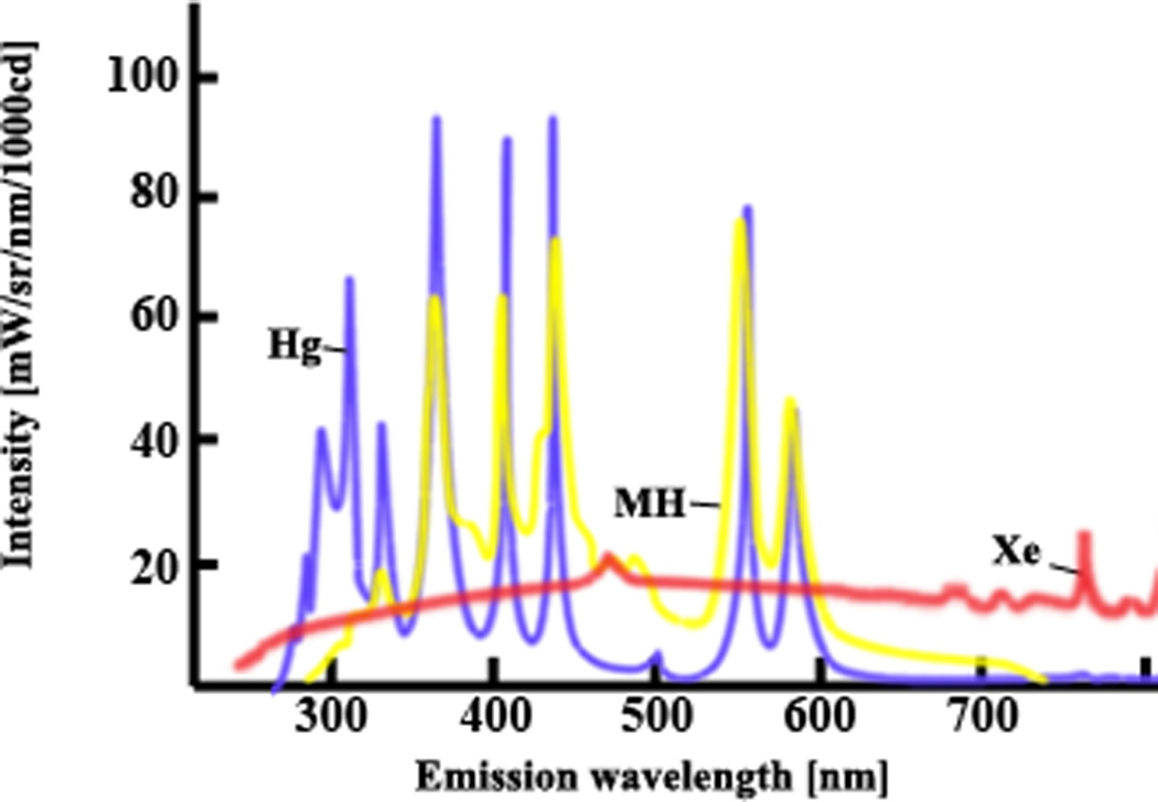
Comparison of spectra of different light. Match the λ_ex of your dyes to a wavelength that is provided strongly by the available illumination source(s). Images used by permission from zeiss.com. Hg: mercury; Xe: xenon; MH: metal halide.

Imaging: Two Guiding Principles

When using dyes, the final images are the data, so ex post facto manipulation to improve images would be altering data. Therefore, the images need to be as good as possible when collected. The GIGO (garbage in, garbage out) principle applies here. To get the best images, use the equipment to the best of its abilities. One important aspect of that is to use the full range of gray levels available – this is essentially the resolution of the image. Once the software is running, shut off any kind of autoscaling feature offered. Autoscaling features will make images look like the full range was used, but it’s a trick, not real data, with that much resolution. So the first thing to do when starting to image is set what you see equal to what you are actually getting. For an 8-bit image, that means set the grayscale image on the screen to go from ± 26 to ± 230. Those numbers come from the number of levels available (2⁸ = 256) minus the extreme 10% at either end. It is important to stay away from the extremes because the software will apply a value of 255 to any pixel that is actually at that intensity, but also to any pixel that is at a higher intensity, that is, saturated and therefore bad data. Likewise, if a pixel is underexposed, it will be given a value of 0 (bad data). The extremes of measuring devices are also the most error prone in general. 10% on each end is a reasonable buffer. Thus, for a 12-bit image, you could set the scale to ± 41 to ± 4055 (2¹² = 4096 minus 10% at each end). Setting the scale may be accomplished using sliders or a menu, depending on the software, and there may be a default setting that you want or need to override.

The other principle at work here is that nothing is perfect. There is always error/uncertainty, and, as good as they are, microscopes are no exception. But there are ways to account for that error, and some very clever ways to minimize it. First, consider all possible sources of error in the whole system. Some fraction of the light emitted by the fluorescent specimen goes through the medium, the coverslip, the air, water, or immersion oil, and into the lenses of the microscope. As it passes through the lenses it may be distorted by imperfections in the glass. Between the charge-coupled device (CCD) camera and the screen, the photons are converted to electrons, and then to numbers interpreted as pixel intensities on the screen and, when you take a picture, in the file generated. That’s a lot of opportunities for error. But, all the light goes through the same set of error generators. So, one can take what are essentially “control” pictures – pictures of just the error – and use them to remove systematic error from your images. Two control pictures are required, a DF image and an FF image (these may be referred to by other names, so judge by how they are made, not by what they are called). A DF control is made by shutting off all light (hence, DF) to the camera and taking a picture. What you get is a picture of electronic noise, and this can be subtracted from your image using the software’s image arithmetic subtraction function (in practice, the DF correction rarely affects the appearance of the image because the dyes are generally bright). An FF control is made by illuminating the specimen, then, using the exact exposure you use to collect data, taking an out-of-focus image of a blank (i.e. flat) place in your sample (such as a region of the slide with no specimen). This is a picture of how the illumination varies across the field of view and how the light is distorted on its way to the camera. The software subtracts the DF control from both the image and the FF control, and then divides the DF-corrected raw data image by the DF-corrected FF image (i.e. normalizes to the FF image). The result is a data image that has had much of the systematic error legitimately removed. It is important to STOP THERE. These two corrections are necessary and sufficient to make the most accurate image of fluorescence intensity. Any more adjusting alters the data. One exception to this rule occurs if the computer draws the ratio image using only a few different intensity levels. This can happen if pixel values in the raw data image and the FF image are close, making the magnitude of the ratio very small – often under 5 (on a 0 to 255 scale). If this happens, it is acceptable to multiply the ratio values by 100 (for 8 bit, 1000 for 12 bit) as long as it is done absolutely consistently. The effect of this transformation is to allow the software to use the significant digits that are to the right of the decimal point; it is the equivalent of making an image of “centi-intensities” rather than intensities.

Because using fluorescent reporters of V_mem and ion concentration is, by definition, a quantitative approach, your images must have these corrections, and no more. Save both your original raw data image and the corrected image. If you plan to export the images for analysis in another software package, be absolutely certain that some default process does not change the data for example, during a change in bit-depth.

In summary, to get the best possible images, set the grayscale of the image to the widest practical range, routinely perform both DF and FF corrections, and make sure neither you nor any software alters the images in any way that alters the data.

Calibration

There are three commonly used calibration techniques that vary in cost, necessary equipment, and accuracy of the results. The gold standard is to simultaneously use dyes and microelectrodes. Unexpected uncertainty may be part of this technique when it is used to measure V_mem, however, since electrodes report average V_mem and therefore miss subcellular differences that might be of importance (see examples below). The second method is to control V_mem/[I] by manipulating the bathing solution with ions and ionophores (which are frequently found in the same sections of catalogues as the dyes; Maher et al. 2007). This technique works quite well for calibrating [I] reporters. It is more problematic for calibrating V_mem reporters because part of this technique is using the Goldman-Katz equation to calculate V_mem based on knowing external and internal ion concentrations, and for most cell types, internal ion concentrations are not known or they vary. The final method is to calibrate the change in V_mem or [I] as a function of the percent change in intensity. This information is usually provided by the supplier (for example, “a 1% change in intensity represents a 1 mV change in V_mem”). This allows some degree of quantification even in the absence of absolute values.

Controls

1. Alter V_mem/[I] using ionophores (control for direction of change in fluorescence intensity). Relevant ionophores are often listed in the same section of catalogues as the dyes.

2. Image undyed cells using identical parameters (control for autofluorescence and phototoxicity of λ_ex).

3. If using two FBRs for V_mem imaging, image cells with only one dye at a time (control for unexpected interactions).

4. Grow the cells in the dye for as long as possible (control for toxicity of dye and/or effect of dye on physiology).

5. Using time-lapse, image the time course of dye uptake and bleaching (control for the timing of imaging relative to staining).

This list is not comprehensive but these observations will provide important information for choosing an FBR/FBR pair that will be useful in your system of interest.

Analysis

Unless you have calibrated your dye, the analysis will be semi-quantitative; that is, you will be able to measure relative differences but not absolute values. The analysis will be done using the software that controls the microscope or any image software that allows you to work with pixel intensity values. You will be comparing corrected signal intensities (see Imaging above) from different parts of single images or from different images from Z or time-series stacks. If you have calibrated your dye, you may also be comparing among different images.

The first step is to do the DF and FF corrections, then, if appropriate, calculate the ratios. Once you are working with fully corrected data images, you will have to use your judgment, or some external standard, to decide how to define regions of interest (ROI), and you should report the criteria. Once you are sure you can minimize bias when choosing ROIs, you will likely be comparing means (± standard deviation, not standard error) of pixel intensity. This calculation is a basic function available in almost every microscopy software package, and most programs have a way to export the numbers to a spreadsheet, but you can always just write them down. Statistical comparisons are easily performed with any basic statistics package. It can also be illuminating to look at histograms of intensity distribution, particular when deciding how to define ROIs. Transects through important structures can also be useful to include in a figure.

Presentation

Figures showing data collected using FBRs should include: representative data images, meaning images that have been fully corrected and the ratio if applicable; appropriate control data; an example of each ROI; the results of any calibration; any standard curve used to interpret the data; the actual results in an appropriate format (probably scatter plots). The materials and methods, results and/or figure legends should include: the full name of the dye; its source; its excitation and emission wavelengths; kd (or pKa) if known; the solvent used for the stock; the working concentration used; the exact filters used for imaging; and the criteria for choosing ROIs.

CONCLUSIONS

As the use of FBRs becomes more widespread, the possibilities and limitations will become better understood and the design of new and better FBRs will continue, and hopefully accelerate. The techniques described here have the potential to open novel and exciting paths of inquiry by significantly extending our ability to measure fundamental and critical aspects of cell physiology. Adding both spatial and temporal information to our knowledge of the bioelectrical processes that interact with biochemical and genetic processes can have enormous impact in both pure and applied biology.

REFERENCES

- Adams DS. A new tool for tissue engineers: Ions as regulators of morphogenesis during development and regeneration. Tissue Engineering Part A. 2008;14(9):1461–1468. doi: 10.1089/ten.tea.2008.0080. [DOI] [PubMed] [Google Scholar]
- Adams DS, Levin M. Measuring resting membrane potential using the fluorescent voltage reporters DiBAC4(3) and CC2-DMPE. Cold Spring Harb Protoc. 2012 doi: 10.1101/pdb.prot067702. [DOI] [PMC free article] [PubMed] [Google Scholar]
- Beane WS, Morokuma J, Adams DS, Levin M. A chemical genetics approach reveals H,K-ATPase-mediated membrane voltage is required for planarian head regeneration. Chem Biol. 2011;18(1):77–89. doi: 10.1016/j.chembiol.2010.11.012. [DOI] [PMC free article] [PubMed] [Google Scholar]
- Blackiston D, Adams DS, Lemire JM, Lobikin M, Levin M. Transmembrane potential of GlyCl-expressing instructor cells induces a neoplastic-like conversion of melanocytes via a serotonergic pathway. Disease Models & Mechanisms. 2011;4(1):67–85. doi: 10.1242/dmm.005561. [DOI] [PMC free article] [PubMed] [Google Scholar]
- Blackiston DJ, McLaughlin KA, Levin M. Bioelectric controls of cell proliferation: ion channels, membrane voltage and the cell cycle. Cell cycle (Georgetown, Tex) 2009;8(21):3519–3528. doi: 10.4161/cc.8.21.9888. [DOI] [PMC free article] [PubMed] [Google Scholar]
- DiFranco M, Capote J, Quinonez M, Vergara JL. Voltage-dependent dynamic FRET signals from the transverse tubules in mammalian skeletal muscle fibers. The Journal of general physiology. 2007;130(6):581–600. doi: 10.1085/jgp.200709831. [DOI] [PMC free article] [PubMed] [Google Scholar]
- Levin M. Large-scale biophysics: ion flows and regeneration. Trends in Cell Biology. 2007;17(6):261–270. doi: 10.1016/j.tcb.2007.04.007. [DOI] [PubMed] [Google Scholar]
- Levin M. Bioelectric mechanisms in regeneration: Unique aspects and future perspectives. Semin Cell Dev Biol. 2009;20(5):543–556. doi: 10.1016/j.semcdb.2009.04.013. [DOI] [PMC free article] [PubMed] [Google Scholar]
- Levin M, editor. The Physiology of Bioelectricity in Development, Tissue Regeneration, and Cancer. CRC Press; 2011. [Google Scholar]
- Maher MP, Wu N-T, Ao H. pH-Insensitive FRET Voltage Dyes. Journal of Biomolecular Screening. 2007;12(5):656–667. doi: 10.1177/1087057107302113. [DOI] [PubMed] [Google Scholar]
- Mazzanti M, Bustamante JO, Oberleithner H. Electrical dimension of the nuclear envelope. Physiol Rev. 2001;81(1):1–19. doi: 10.1152/physrev.2001.81.1.1. [DOI] [PubMed] [Google Scholar]
- Sundelacruz S, Levin M, Kaplan DL. Role of membrane potential in the regulation of cell proliferation and differentiation. Stem Cell Rev and Rep. 2009;5(3):231–246. doi: 10.1007/s12015-009-9080-2. [DOI] [PMC free article] [PubMed] [Google Scholar]
- Tsutsui H, Karasawa S, Okamura Y, Miyawaki A. Improving membrane voltage measurements using FRET with new fluorescent proteins - Supplements. Nat Meth. 2008;5(8):683–685. doi: 10.1038/nmeth.1235. [DOI] [PubMed] [Google Scholar]
- Tyner KM, Kopelman R, Philbert MA. "Nanosized voltmeter" enables cellular-wide electric field mapping. Biophys J. 2007;93(4):1163–1174. doi: 10.1529/biophysj.106.092452. [DOI] [PMC free article] [PubMed] [Google Scholar]
- Vandenberg LN, Morrie RD, Adams DS. V-ATPase-dependent ectodermal voltage and pH regionalization are required for craniofacial morphogenesis. Dev Dyn. 2011a;240:1889–1904. doi: 10.1002/dvdy.22685. [DOI] [PMC free article] [PubMed] [Google Scholar]