Individualized Statistical Learning from Medical Image Databases: Application to Identification of Brain Lesions

Abstract

This paper presents a method for capturing statistical variation of normal imaging phenotypes, with emphasis on brain structure. The method aims to estimate the statistical variation of a normative set of images from healthy individuals, and identify abnormalities as deviations from normality. A direct estimation of the statistical variation of the entire volumetric image is challenged by the high-dimensionality of images relative to smaller sample sizes. To overcome this limitation, we iteratively sample a large number of lower dimensional subspaces that capture image characteristics ranging from fine and localized to coarser and more global. Within each subspace, a “target-specific” feature selection strategy is applied to further reduce the dimensionality, by considering only imaging characteristics present in a test subject’s images. Marginal probability density functions of selected features are estimated through PCA models, in conjunction with an “estimability” criterion that limits the dimensionality of estimated probability densities according to available sample size and underlying anatomy variation. A test sample is iteratively projected to the subspaces of these marginals as determined by PCA models, and its trajectory delineates potential abnormalities. The method is applied to segmentation of various brain lesion types, and to simulated data on which superiority of the iterative method over straight PCA is demonstrated.

1. Introduction

Voxel-based morphometry (VBM) type of analyses are being increasingly adopted for characterizing neuroanatomical differences between brain images (Ashburner and Friston, 2000; Mechelli et al., 2005). VBM has emerged as an alternative to region of interest (ROI) based approaches. Different brains are compared on voxel-by-voxel basis after being spatially normalized to a common template space. Voxel-wise statistical tests are performed on each individual voxel for a normal population, and voxels that differ from the normal population are flagged and grouped into clusters reflecting pathology, over the entire group, albeit not necessarily at the individual level. A fundamental limitation of this kind of approaches is that it relies on voxel-by-voxel comparisons, and cannot capture more complex imaging patterns.

Voxel-based approaches have also been used in supervised frameworks for segmenting brain lesions. These methods use manually-segmented images annotated by experts, and learn a predictive model from positive and negative training samples obtained from individual voxels with known class labels. Voxel intensities (or values derived from intensities) from single or multiple image channels are used as features that characterize each individual voxel, and a classifier (e.g. kNN, SVM (Burges, 1998; Cortes and Vapnik, 1995)) is trained on these feature vectors (Anbeek et al., 2004; Lao et al., 2008).

Atlas-based methods have been proposed as a way of including spatial context information in lesion segmentation (Prastawa et al., 2004; Shiee et al., 2010; Van Leemput et al., 2001; Wu et al., 2006). A statistical atlas provides the prior probability of each voxel to belong to a particular healthy tissue type. In Prastawa et al. (2004) the atlas is used for sampling voxels from each healthy tissue type. A robust estimator is then used for estimating the probability density function (pdf) of the healthy brain tissue intensity. Brain tumors are segmented as outliers of the estimated pdf. Similarly, in Van Leemput et al. (2001) the parameters of a stochastic tissue intensity model for normal brain are estimated, while simultaneously detecting lesions as voxels that are not well explained by the model. An atlas is used for prior classification of image voxels into tissue types. In both approaches, tissue specific intensity models are used for estimating the normal variation, and the spatial context information is independently used as a prior.

In this paper, we propose a multi-variate pattern analysis method for segmenting abnormalities. Instead of analyzing voxels individually or estimating intensity distributions of healthy tissue types, we basically aim to learn the statistical variation of the healthy brain anatomy in the high dimensional space, i.e. to estimate the pdf of all image voxels, from a training database of normal brain scans¹. Rather than classifying image voxels independently as normal or abnormal, the proposed method detects patterns of abnormality by projecting an image into the hypervolume of normals as defined by statistical models learned from the training samples. We don’t make any assumption about the characteristics of the abnormality, however we assume that normal anatomy follows specific patterns and certain aspects of its statistics can be estimated from a number of representative examples. The method is not specific to a given type of pathology, and thus, it does not require training for many possible types of abnormalities, which is often not practical or even possible, particularly when the pathology is variable and/or unknown in advance.

An important challenge of multi-variate analysis on image data is the problem of high-dimensionality and small sample size. For example, a typical MRI scan of the brain includes several millions of measurements on respective voxels. Moreover, the structure and function of many organs, particularly of the brain and the heart, are very complex and difficult to summarize with a small number of variables extracted from such images. Finally, pathology can cause even more complex and subtle changes in the imaging characteristics, thereby rendering it extremely difficult to train an algorithm to find such changes, without knowing in advance what features to look for. Even though the complexity of the problem would call for thousands of scans to be used as training examples, typical imaging studies often offer just one or two hundred scans for training, or even less. Learning algorithms therefore are limited with respect to the complexity of image patterns they can learn, and the precision with which they can learn them and identify them in new images. We focus on addressing the challenges of such direct estimation of statistical variation.

A common approach to learning from an image database involves some form of dimensionality reduction, such as principal component analysis (PCA) or some sparse decomposition of the training examples, so that a relatively small and manageable set of “features” is extracted from the training data. These features then define the feature space within which each image is projected, prior to building statistical models that estimate its characteristics. If a number of normal brain MRI scans is available, PCA can be used to approximate the statistical distribution of these images, under Gaussianity assumptions. When a new image is presented, its location within the PCA subspace is determined via projection to the principal eigenvectors. Normality or abnormality of the test image can be evaluated by calculating its respective likelihood, given the PCA model of the training set. Similarly, the pattern of abnormality can be estimated by projecting the test image to the subspace of normal brain images, as determined by the PCA. However, the dimensionality of the PCA space is bounded by the number of training samples. Consequently, a PCA model of the whole brain obtained from a limited number of training samples can only capture relatively global patterns of variation in the data.

In order to overcome the small sample size limitation, building upon prior work (Erus et al., 2010), we first propose to sample a large number of lower dimensional subspaces, each of which is sufficiently small relative to the underlying image variations and the available sample size. In the experiments herein, each of these subspaces represents image patches, albeit it does not necessarily have to. The subspaces are derived in a multi-scale fashion, and capture image characteristics ranging from fine and localized to coarser and relatively more global. We impose conditions that allow the statistical variations of these subspaces to be reliably estimated from the available training data. The main premise here is that, an imaging pattern that is consistent with a large number of marginal pdfs, is likely to be consistent with the overall pdf, which has not been explicitly estimated due to the high image dimensionality.

We further reduce the dimensionality within each image patch by applying an individualized feature selection strategy. Learning methods generally try to find the features that best represent the entire set of training examples and their variability. We propose an alternative approach based on a “target specific” feature selection strategy. When the goal is to analyze a specific test image, called the “target”, not belonging to the training image database, the optimal feature extraction and dimensionality reduction for classification of the target image is not necessarily the one that is optimal for the entire training set, but one that best learns the features that are relevant for the specific target image. For example, instead of attempting to learn a statistical model or classifier that reflects all possible variations of normal brain anatomy, we only need to learn the variations of the specific anatomical features encountered in the target brain. Such target-specific learning improves our ability to learn from a database of examples, as it focuses on the features that are present in the specific target being analyzed. These features, of course, are different for different target images. In our experiments, a smaller set of target-specific features are selected within each image patch through an approach based on wavelet thresholding (Donoho, 1995), since it is a method that has been very successful in dimensionality reduction of images and signals. However other sparse decompositions can be readily used instead (Sjostrand et al., 2007). Typically, a small number of features, or expansion coefficients, is necessary to construct the main characteristics of a target image.

The validation experiments are applied on FLAIR (FLuid Attenuation Inversion Recovery Magnetic Resonance Imaging)-MRI images, for the segmentation of two types of abnormalities with different signal and spatial characteristics: white matter lesions and cortical infarcts. We evaluate the segmentation accuracy on both simulated and real abnormalities. WMLs show up as hyperintensities with respect to surrounding healthy white matter (WM) tissues on FLAIR images. An infarct is generally the result of a stroke that occurs when the blood supply to the brain is interrupted, due to cerebrovascular disease (CVD). It consists of necrosis, i.e. a region of dead brain tissue, typically surrounded by a rim of tissue that is not dead but not entirely healthy, either. Many clinical studies investigating CVD require segmentation of the necrosis (Barkhof, 2003). The accurate segmentation of these regions is difficult as their intensity patterns are similar to the adjoining cerebrospinal fluid (CSF).

The paper is organized as follows: Section 2 describes the proposed method. The experimental results are given and discussed in section 3. Section 4 summarizes and concludes with additional discussions and future perspectives.

2. Method

Consider medical images of a normative population coregistered to a common domain Ω as realizations of a d-dimensional random vector I, consisting of d scalar random variables [x₁, x₂, …, x_d] corresponding to intensities of the image voxels. The joint pdf of I,

$$\varphi (I)=\varphi (x_1,x_2,..,x_d)$$ (1)

describes the relative likelihood for I to be observed. Images for which ϕ(I) ≥ t lie in a hypervolume, which (for the purposes of this paper in which we consider anatomical brain images) we call the subspace of normal anatomy, in the d dimensional space. For any given test image to be compared with the normative population, if we can estimate ϕ( ), the likelihood of being abnormal can be calculated. Also, if is abnormal, , the most similar image to that is within normal variation, can be obtained by projecting to this hypervolume. The difference between and provides an image of the abnormality patterns in . In most practical applications, however, ϕ(I) is unknown, while only a small set of n ≪ d training samples is available for estimating it.

Estimating ϕ(I) is a challenging problem, particularly when d is very high. Furthermore, the underlying distribution of the data is generally unknown. Previous studies have shown that images of complex objects, e.g. faces, brains, lie on a lower dimensional nonlinear submanifold embedded in the high dimensional space. In the machine learning literature, many manifold learning methods, which aim to capture the low dimensional manifold structure from the data samples in the high dimensional space, have been proposed (Roweis and Saul, 2000; Tenenbaum et al., 2000). Recently, manifold learning methods based on diffeomorphic deformations are used in Gerber et al. (2010) and Hamm et al. (2010) for representing brain images. However, nonlinear models are difficult to estimate, and require a large number of samples for learning the underlying manifold structure. For this reason, we take a different approach, motivated by our primary aim being to detect abnormalities in a test image. In particular, we sample from the image domain a large number of lower-dimensional subspaces, and estimate the distribution of the data by estimating pdf s of each subspace using a linear model, assuming that regional imaging statistics can be approximated to a large extent by Gaussian distributions. The likelihood of a new image is evaluated by testing the likelihoods of its projections to the smaller subspaces in order to detect patterns of abnormality on it. An image of potential abnormalities is formed by an iterative procedure that finds a path from to the normal hypervolume.

While ϕ(I) can not be estimated accurately from a limited number of training images, if a subspace is small enough, the pdf of the image projection on it can be estimated more reliably. If the projection is selection of certain voxels, effectively, this would estimate the marginal pdf involving those voxels. Assume that a large number of partially overlapping subspaces S = {ω₁, …, ω_r} are sampled from Ω, where

$$\mathrm{\Omega }=\cup {\omega }_i,i\in \{1,\dots ,r\},$$ (2)

with a high degree of redundancy, i.e., each voxel is included in many ω_i’s.

The likelihood of a new test image’s projection ${\mathcal{I}}_{\omega }^t$ to a subspace ω ∈ S can be calculated by estimating the pdf $\varphi (I_{\omega }^t)$ using the set of n training samples. This estimation is defined according to the statistical modeling approach used herein. From , an image without abnormalities (i.e. an image that represents the closest point in the hypervolume of normals according to the estimated subspace models) can be reconstructed by minimizing the following energy function:

$$E({\mathcal{I}}^{\ast })={\Vert {\mathcal{I}}^{\ast }-{\mathcal{I}}^t\Vert }_{l_2}^2+\alpha \sum _{i=1}^{r}L({\mathcal{I}}_{{\omega }_i}^{\ast })$$ (3)

The data term reflects the image dissimilarity, computed as the l₂-norm of the difference between the test image and the reconstructed image. The model term reflects the likelihood of being abnormal according to the subspace model, i.e. L is the abnormality term that indicates how abnormal an image with respect to the subspace model learned from the normals, and it’s defined as:

$$L(I)=\{\begin{array}{ll}0\hfill & \text{if}M(I)<t\hfill \\ M(I)-t\hfill & \text{otherwise}\hfill \end{array}$$

where M (·) is the Mahalanobis distance, and t is the threshold for normality, such that images within the normal ellipsoid around the mean of the training data are considered as normal.

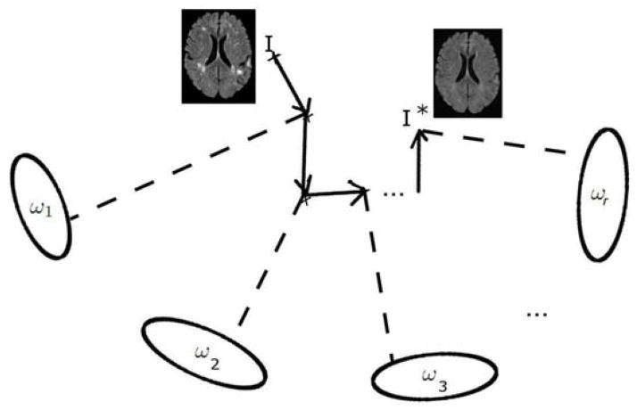
For solving eq. 3, we use an iterative strategy employing a technique similar to block-coordinate descent, where in order to minimize a multivariable function, optimization with respect to different (smaller) subsets of variables is iteratively achieved. We calculate the optimal reconstruction for one image subspace ω_i at a time, and iterate over a large number of subspaces (Figure 1). The local solution in each subspace could have been fused into a globally optimal estimate that satisfies the overlap constraints by applying a distributed estimation algorithm as performed in Zacharaki and Bezerianos (2011). However, the application of this method to 2D data showed that there is no significant improvement over our iterative approach, while the memory requirements for such a joint optimization scheme hinders its application to real 3D data.

Figure 1.

Illustration of the iterative reconstruction of the normal. At each iteration step, the image is constrained to be normal according to one subspace model.

2.1. Subspace representation

S may be obtained in various ways. Generally speaking, an image subspace may consist of any subset of arbitrary image voxels or set of values derived from image voxels. Here we limit ourselves to rectangular image patches of varying sizes, which correspond to local neighbourhoods around voxels in different spatial positions. Neighbouring voxels are highly correlated in natural images, and the intrinsic dimensionality of image patches is generally much lower than their actual dimensionality, which makes them more reliably estimable.

An image patch consists of voxels in a rectangular block of size s_i ∈ ℜ³ around a selected seed voxel location l_i ∈ ℜ³. At each iteration i, a patch is drawn from Ω by random selection of the seed location and the patch size. An edge detector (Canny, 1986) is first applied on to restrict the set of all possible seed locations, , to voxels with relatively richer information content. To make sure that the space is well sampled, a weighted random selection strategy is used. A weight value is assigned to each l ∈ , and the selection is done such that l has a probability of being selected proportional to its weight. Initially, an equal weight value is assigned to each l. At the end of each iteration, the weights of all l ∈ that are within the selected image patch are decreased by a constant factor, so that these voxels will have a lower probability of being selected in subsequent iterations, to encourage this process to sample the entire domain fairly evenly.

Block size s_i varies randomly in an interval bounded by predefined minimum and maximum values. In that way, the set of all subspaces capture image characteristics ranging from fine and localized to coarser and relatively more global at different spatial locations of the image domain.

2.2. Target specific feature selection

We use a target-specific feature selection strategy, i.e. a strategy that aims to estimate from the training set only those imaging aspects that are necessary to process the test image (i.e. the target). The feature selection method first expands the test image patch in a basis that better allows us to determine the important components of it, and then selects an estimable subset of these components for statistical group analysis.

Feature selection is based on wavelet transform. A detailed exposition of wavelet based compression techniques is available in Donoho (1995) and Mallat (2008). A wavelet transform produces as many coefficients as there are voxels in the image. However, it provides a more compact representation, such that most of the information is concentrated in a small fraction of the coefficients. Also, wavelet coefficients with larger magnitude are correlated with salient features in the image data. The compression is performed by applying a thresholding operator to the coefficients in order to select a subset of coefficients with the largest values.

Let d^t be a vector of voxel intensities extracted from image patch ω on , and ${\mathbf{d}}_i^{\mathit{Train}}$, i ∈ {1, .., n} be the voxel intensities from the same patch on each training image. By applying a wavelet transform, d^t may be represented as a linear combination of several predefined wavelet basis functions:

$${\mathbf{d}}^t=\sum _{j=1}^m{\mathrm{a}}_j{\mathit{\psi }}_{\mathbf{j}}$$ (4)

where a_j are wavelet coefficients sorted in descending order of absolute value, ψ_j are the corresponding wavelet basis functions, and m is the dimensionality of d^t (the number of voxels in the image patch). This allows us to choose the p basis functions with largest coefficients (p < m) and write

$${\mathbf{d}}^t=\sum _{j=1}^p{\mathrm{a}}_j{\mathit{\psi }}_{\mathbf{j}}+{\mathcal{R}}^t$$ (5)

where is the residual. The feature vector

$${\mathbf{a}}^t\doteq {\{{\mathrm{a}}_j\}}_{j=1}^p$$ (6)

can be used to reconstruct the image after wavelet thresholding. In our application, we apply an iterative algorithm for determining p: starting from p = m, the value of p is decreased gradually until the selected coefficients satisfy the estimability criterion (discussed in a subsequent section), which reflects whether the corresponding pdf of these coefficients can be estimated from the training normal data. In this way we select the largest set of coefficients whose pdf is estimable. p takes different values for different image patches, but it always satisfies m > p > n.

Note that the basis wavelets ${\{{\psi }_j\}}_{j=1}^p$ are selected based on the target data only. Each training image patch ${\mathbf{d}}_i^{\mathit{Train}}$ is projected to the selected basis:

$${\mathbf{d}}_i^{\mathit{Train}}=\sum _{j=1}^p{\mathbf{A}}_{ij}{\mathit{\psi }}_{\mathbf{j}}+{\mathcal{R}}_i^{\mathit{Train}}$$ (7)

to obtain the training feature matrix A ∈ ℜ^n×p, which has, in each row, p wavelet coefficients from each training image patch.

2.3. Statistical model constrained reconstruction within a subspace

Various modeling approaches may be used for estimating the pdf of the selected features. We applied PCA, an orthogonal linear transformation, where a number of principal components that account for as much of the variability in the data as possible are calculated, based on the assumption that the data follow a Gaussian distribution. One of our assumptions here is that regional statistics can be approximated by Gaussian distributions, even if the distribution of the entire image is highly non-Gaussian.

Let A ∈ ℜ^n×p be the data matrix, consisting of feature vectors obtained from n training samples. Let ā ∈ ℜ^1×p be the mean of the rows of A. The mean-centered data matrix B ∈ ℜ^n×p is computed by subtracting ā from each row of A. Let C ∈ ℜ^p×p be the sample covariance matrix of B. An eigenvalue decomposition is applied to calculate λ, the vector of n − 1 nonzero eigenvalues of C sorted in descending order, and Q ∈ ℜ^p×(n−1), the first n − 1 eigenvectors of C.

When projected to the space spanned by Q, a data vector a^t ∈ ℜ^1×p, which consists of the coefficients selected from the target image, can be represented by its projection vector v:

$$\mathbf{v}={\mathbf{Q}}^T{({\mathbf{a}}^t-\overline{\mathbf{a}})}^T.$$ (8)

As the application of PCA diagonalizes the covariance matrix C, the pdf of a^t can be computed by

$$\varphi ({\mathbf{a}}^t)=\varphi (\mathbf{v})=c\mathit{exp}\{-\frac{1}{2}\sum _{j=1}^{n-1}\frac{v_j^2}{{\lambda }_j}\},$$ (9)

where c is the normalization coefficient, and v_j and λ_j are the j^th elements of v and λ respectively. Consequently, an image patch that has a low likelihood can be constrained to have a desired likelihood t on the PCA subspace by scaling down its projection coefficients by a scalar factor q

$${\mathbf{v}}^{\ast }=q\mathbf{v}s.t.\varphi ({\mathbf{v}}^{\ast })=t$$ (10)

The reconstructed data vector a^* can be obtained by projecting v^* back to the original space:

$${\mathbf{a}}^{\ast }={({\mathbf{Qv}}^{\ast })}^T+\overline{\mathbf{a}}.$$ (11)

Estimability of a subspace

We aim to select features whose respective pdf ’s are reliably estimable from the limited set of training data. We consider that the pdf of the feature vector derived from a subspace is estimable if a significant fraction γ_v of the overall variance of the data can be explained by a small fraction γ_e of eigenvectors. The thresholds γ_v and γ_e are parameters to be chosen based on the particular application. Normalized eigenvalues

$$\widehat{\mathit{\lambda }}=\mathit{\lambda }/\sum _{j=1}^{n-1}{\lambda }_j$$ (12)

represent the fraction of variance contributed by each eigenvector. We calculate

$$\xi =(\underset{x\in \{1,\dots ,n-1\}}{argmin}\sum _{j=1}^x{\widehat{\lambda }}_j\ge {\gamma }_v)/(n-1)$$ (13)

A feature vector is considered estimable if ξ < γ_e.

2.4. Generation of voxelwise abnormality maps

Training and testing MRI images were first pre-processed using a standardized pipeline including skull stripping using the BET algorithm implemented in FSL software library (Smith, 2002) and bias correction using N3 (Sled et al., 1998). In order to eliminate intensity variations due to scanner differences a global histogram matching, between the image histogram and the histogram of a common template image, is applied using an in-house technique. The method calculates optimal translation and scaling values {h_t, h_s} that are applied on the subject image’s histogram to make the model image histogram and translated and scaled subject image histogram similar. Specifically, we search for:

$$\underset{h_t,h_s}{argmin}{\Vert H_M-(H_S-h_t)/h_s\Vert }_2$$

where H_M is the histogram of the model image, H_S is the histogram of the subject image, and || · ||₂ is the l₂ norm.

Histogram matched images are coregistered to the common template using a non-linear registration algorithm that is robust to the presence of abnormalities, since it uses the concept of attribute vectors (Shen and Davatzikos, 2002). The registration aims to preserve the anatomical variation to a certain extent, and most importantly not to force the abnormal areas to match the healthy anatomy. For this reason, we applied HAMMER with a parameter setting that would result in a smooth deformation field. The specific parameter values are deformation field smoothing factor c = 0.5 and E = 30 iterations of edge preserving smoothing.

The overall procedure for minimizing the energy function defined in eq. 3 is applied on each test image , and the closest image being part of normal variation without pathology, , is obtained. An intensity abnormality map, , is computed as the voxelwise difference between and . Voxel values on reflect the amount of abnormality, measured as the difference between observed signal intensity and the estimated normal intensity according to the method. Since different brain regions display different levels of image variations, we adaptively normalized the abnormality map for the test sample at each voxel using abnormality values obtained from the training samples. Specifically, for each training image an abnormality map is computed using the proposed approach with leave-one-out cross validation. At each voxel, the mean and standard deviation of the abnormality values from all training samples is calculated. is normalized by calculating the standard (z) score of the raw abnormality score at each voxel, with respect to the distribution estimated from the training data.

3. Experimental results

We conducted several experiments with the proposed method on various datasets using different settings. A first experiment on simulated data with high dimensionality and low sample size compared projections to normal subspace using a single PCA model against using the iterative PCA approach. In our experiments on brain MRI images, we first explored the accuracy of the reconstruction within each subspace, i.e. on single image patches, by reconstructing image patches extracted from different locations of the brain, and segmenting simulated abnormalities on these patches. We then investigated the convergence of the reconstruction with each iteration, and the effect of parameters such as the block size and the likelihood threshold t on the reconstruction through a set of experiments using 2-dimensional axial slices. Finally, we applied our method for segmenting lesions and infarcts on 3-dimensional MRI images.

3.1. Iterative reconstruction on simulated distributions

We first investigated experimentally the validity of our main premise that motivated the iterative approach: estimation of a large number of marginal pdf s through projections to image subspaces in order to estimate the global pdf.

With this aim, a k-dimensional multi-variate normal distribution ~ (μ, Σ) with known mean μ ∈ ℜ^k and covariance Σ ∈ ℜ^kxk is simulated. A set of n training samples, such that n ≪ k, are sampled from this distribution. In this experiment, we set k = 3000 and n = 50. Testing samples, i.e. abnormal data deviating from the distribution, are generated by randomly sampling data points from a distribution with mean μ and the covariance 3 * Σ, and selecting 10% of the samples with the highest Mahalanobis distance. For each test sample p, the optimal normal point p̂, i.e. the closest point that is considered normal according to is computed, using the average Mahalanobis distance of the training samples as a cut-off value between normal and abnormal data.

The iterative reconstruction approach over smaller dimensional data subspaces is compared to a projection using a single PCA on the whole data domain. The iterative approach is applied on randomly selected subsets of dimension d = 100 for t = 300 iterations. The reconstruction error $r={\mid {\mathbf{p}}^{\ast }-\widehat{\mathbf{p}}\mid }_{l_2}^2$, i.e. the distance between the reconstructed (p^*) and optimal (p̂) normal points, is calculated for all test samples for both approaches. Figure 2 shows the histogram of the reconstruction errors for 50 test samples for both experiments. We observed that the iterative approach outperformed the single PCA approach in recovering the optimal normal data point. The evolution of the reconstruction error through each iteration for a randomly selected test sample is given on figure 3.

Figure 2.

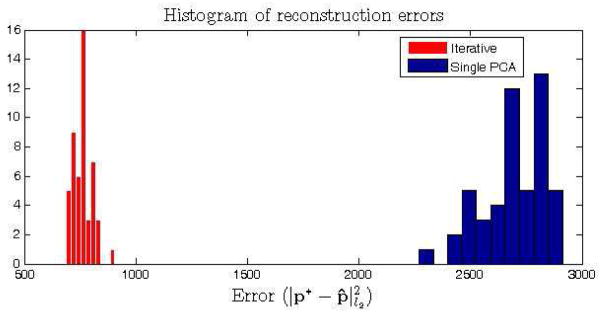
Reconstruction of the normality on simulated data. Histogram of the reconstruction errors for 50 test samples using the iterative and single PCA approaches.

Figure 3.

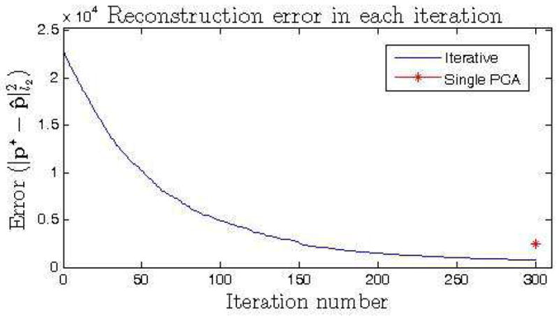
Reconstruction of the normality on simulated data. Evolution of the reconstruction error at each iteration for a randomly selected test sample. The reconstruction error at the final iteration is compared to the error by the single PCA approach.

3.2. Segmentation of abnormalities on MRI images

MRI allowed noninvasive visualization and characterization of structural brain abnormalities for clinical diagnosis of brain pathologies. In our validation experiments, we specifically focused on automatic segmentation of white matter lesions, cortical infarcts, and periventricular atrophy, as these are three types of common abnormalities of the brain that exhibit different MRI signal characteristics and occur in different spatial locations of the brain. On FLAIR images WMLs show up as hyperintensities with respect to surrounding healthy white matter tissue. Cortical infarcts have a necrotic part in the cortex surrounded by a hyperintense rim. The necrotic part of the infarct generally has an intensity profile similar to the cerebrospinal fluid (CSF). The periventricular atrophy is the enlargement of the ventricles as a result of the atrophy in surrounding brain tissue. Examples of images with each type of abnormality are shown in figure 4.

Figure 4.

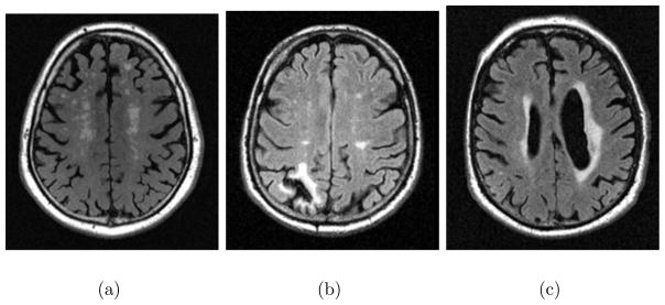
Axial views of FLAIR images showing examples of each type of abnormality targeted in the validation experiments, a) White matter lesions, b) cortical infarct, c) periventricular atrophy and lesions.

FLAIR MRI scans from 73 healthy subjects, with voxel dimensions 0.93, 0.93 and 3 mm. in x, y and z axes, are used as the training dataset in our experiments for learning the normality. All training scans are visually verified so that they don’t include any visible pathologies. The method is validated on two independent test sets: Set1 involved images of 33 diabetic patients with generally high total load of WMLs; Set2 consisted of 47 images selected from an ageing population based on high prevalence of abnormalities. The average age of the training subjects was 59.3 with a standard deviation of 4. The testing subjects had average age 61.2 ± 5.6, and 75.02 ± 4.73 respectively. Manual WML masks have been drawn by a radiologist on Set1. On Set2 manual masks for WMLs and infarcts were created by two raters trained by a radiologist.

3.2.1. Reconstruction of a single image patch

We first investigated the capacity of the wavelet PCA model to capture the variation of the healthy brain anatomy within a single image patch. Abnormalities simulated on selected image patches are used for evaluating how good the healthy brain is reconstructed.

From the preprocessed training images, a subset of 5 random images is selected as the testing set, and the remaining images are used as the new training set. Two dimensional image patches of size 50 by 50 voxels are extracted from 3 different anatomical locations of the brain, cortical, periventricular and deep white matter. Simulated abnormalities (hypointense or hyperintense) have been created by increasing or decreasing the intensity value of voxels within a circular area around a randomly selected seed location on the patch, by a variable offset value o_i ∈ ±{10, 15, 20, 25, 30, 35, 40, 45} that corresponds to 4 to 18% of the intensity range of the template image, whose intensity values were linearly mapped to [0, 255]. Corresponding binary ground truth masks are generated for validation. Examples of simulated abnormalities on two patches from the cortical and periventricular regions are shown in figure 5.

Figure 5.

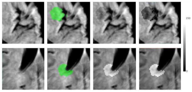
Examples of simulated abnormalities on image patches; hypointense on cortical (first row), hyperintense on periventricular (second row). Left to right: Image patch, ground-truth mask overlaid on the image, simulated abnormality with an offset value of ±20, simulated abnormality with an offset value of ±40.

For each test sample, a single iteration of the method is applied by selecting the entire test patch as the target. The estimability parameters are set to γ_v = 0.8 and γ_e = 0.25 (at least 80 % of the variance can be explained by 25 % of the principal components for an estimable subspace).

We first visualized for each location, the first three eigenvectors with highest eigenvalues that are calculated from the selected wavelet coefficients by transforming them back to image domain for visualization. As shown in figure 6 the eigenvectors successfully captured the general patterns of anatomical variation across subjects around the sulci and the ventricles. As expected, the quite regular variation pattern around the ventricles is captured in few eigenvectors and thus the final estimable set of selected wavelet coefficients was large (939 wavelet coefficients in average) compared to cortical regions (184 wavelet coefficients selected in average), that were more difficult to estimate due to higher anatomical variation.

Figure 6.

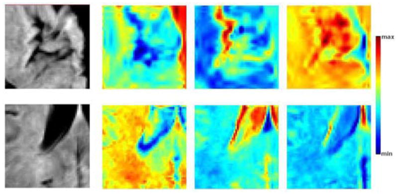
First three eigenvectors for cortical (top) and periventricular (bottom) patches. Leftmost, sample image patch from the training set; from left to right, the most significant eigenvectors in order of significance. The eigenvectors for the cortical patches explain 32.5, 7.5 and 5.9 % of the total variation, those for the periventricular patches explain 34.9, 11.2 and 6.3 % of the total variation. The colormap is stretched to the min. and max. values of each eigenvector for visualization purposes.

We evaluated the segmentation accuracy by calculating the Area Under the Curve (AUC) value for the overlap between the abnormality maps and the ground-truth masks. Figure 7 presents the average AUC scores for the segmentation of simulated abnormalities on each anatomical location for different intensity offset values. The method could successfully segment abnormalities, particularly those with more than 8% change from the normal tissue intensity value. The hyperintensities and abnormalities in non-cortical regions were segmented with higher accuracy. Thresholded abnormality maps obtained for two samples with cortical hypointensities and periventricular hyperintensities are shown in figure 8.

Figure 7.

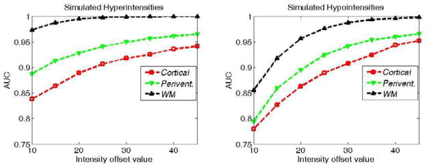
Average AUC scores for the segmentation of simulated hyper and hypo-intensities for each intensity offset value.

Figure 8.

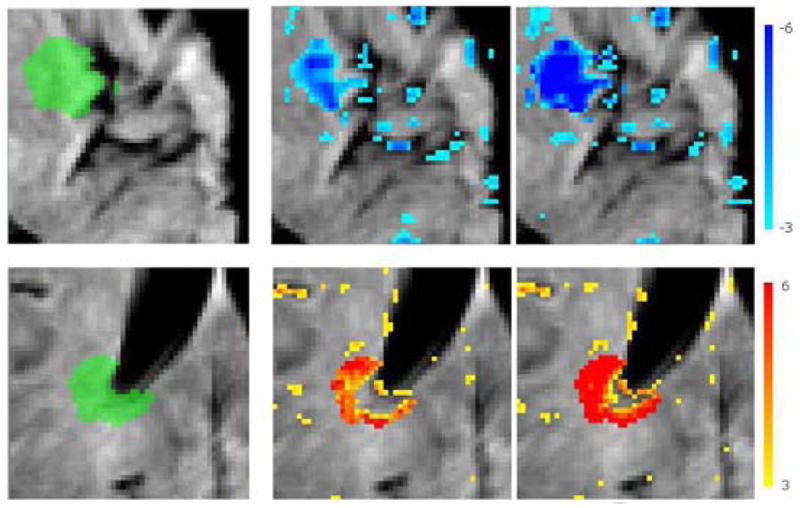
Thresholded abnormality maps for simulated abnormalities on cortical (top) and periventricular (bottom) patches. Left: Ground-truth mask, middle: abnormality map for intensity offset values ±20, right: and ±40

3.2.2. Analysis of sensitivity to block size and likelihood threshold

On a set of selected axial slices of the images from 5 healthy subjects we simulated a variable number of abnormalities, i.e. hyperintense and hypointense areas in randomly selected image locations with different sizes and shapes. Specifically: 5 locations were selected for each subject in average; the abnormalities had a circular-like shape with random perturbations on the boundaries, with intensity difference to normal tissue decreasing from the center to the boundaries; the radius of abnormalities were between 5 to 8 mm.; the average intensity in the selected area was increased or decreased each time by values varying between 4 to 16% of the intensity range of the template image.

We investigated the segmentation accuracy and reconstruction error on the whole image, using different values for the patch size range (s_i ∈ { [15, 20], [20, 25], [25, 30], [30, 40], [5, 40]}, with t = 2, γ_v = 0.8 and γ_e = 0.25), and the likelihood threshold (t ∈ {1, 1.4, 1.8, 2.2, 2.6}, with s_i = [15, 20], γ_v = 0.8 and γ_e = 0.25). The method is run for 1000 iterations in each experiment. The reconstructed image and the final abnormality map are kept in every 20 iterations, and two metrics are calculated to evaluate the reconstruction: The l₂ norm of the voxelwise difference between the reconstructed image and the original image (without simulated abnormalities), and the AUC value for the agreement between the ground truth abnormality mask and the abnormality map computed by the method.

The values of the final evaluation metrics for each set of experiments are shown in figures 9 and 10. In both set of experiments both metrics converged to a stable value with almost all parameter values after a few hundred iterations. On initial iterations, the accuracy of the abnormality segmentation was highest using a low t (figure 9, left), i.e. one that defines a smaller hypervolume for the normality, possibly because the test image was more aggressively changed based on training data; however with more iterations the same accuracy was obtained with higher values of t, while also achieving a lower reconstruction error on the healthy parts of the brain(figure 9, right). The method had comparable final segmentation accuracy for ranges including large (> 20) blocks (figure 10, left). The convergence to optimal accuracy was faster with the block size range [30, 40], which also obtained a significantly lower reconstruction error compared to other parameter values. While the segmentation accuracy is not very sensitivity to block size (as long as blocks large enough to contain both the abnormality and surrounding normal regions are allowed), for accurate reconstruction of the normal tissue the block size should be carefully selected with respect to the size of the available training sample.

Figure 9.

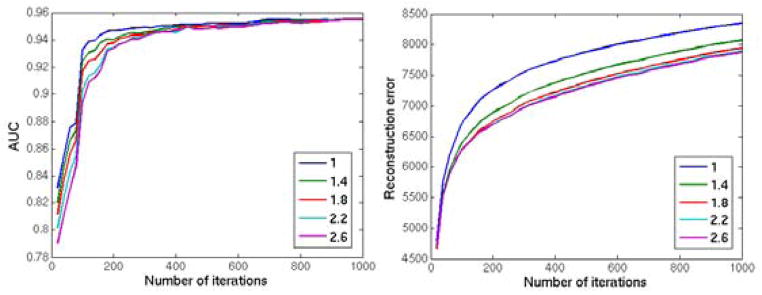
Reconstruction of the 2 dimensional image with simulated abnormalities using different parameter values of the likelihood threshold t ∈ {1, 1.4, 1.8, 2.2, 2.6}. Left: The AUC value for the agreement between the ground truth abnormality mask and the abnormality map computed by the method; Right: The l₂ norm of the voxelwise difference between the reconstructed image and the original image. The method is applied for 1000 iterations and the results are calculated in every 20 iterations.

Figure 10.

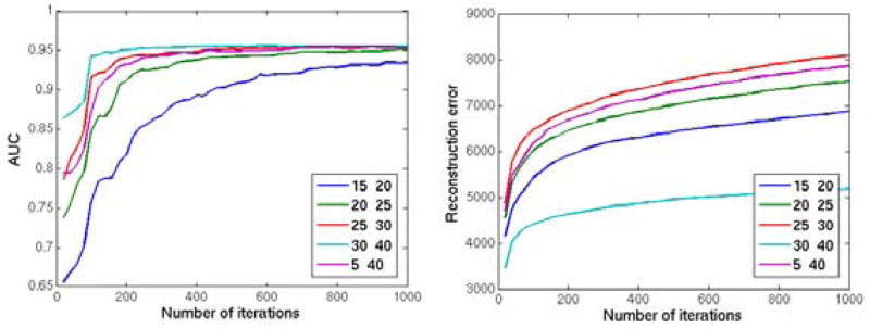
Reconstruction of the 2 dimensional image with simulated abnormalities using different parameter values of the patch size range (s_i ∈ {[15, 20], [20, 25], [25, 30], [30, 40], [5, 40]}. Left: The AUC value for the agreement between the ground truth abnormality mask and the abnormality map computed by the method; Right: The l₂ norm of the voxelwise difference between the reconstructed image and the original image. The method is applied for 1000 iterations and the results are calculated in every 20 iterations.

3.2.3. Abnormality segmentation

For each test sample the proposed method is applied on the whole image using all training images as the training set. The block size is set to vary between 10 to 30 in x and y axes, and between 4 to 8 in z axis, taking into consideration the lower resolution in z axis, and particularly aiming to generate axial image patches large enough to include whole abnormalities. The estimability parameters are set to γ_v = 0.8 and γ_e = 0.25, and the likelihood threshold to t = 2. A final abnormality map is calculated for each test image. Two abnormality maps are then extracted from this map, one by including only voxels with positive differences, and the other by including voxels with negative differences. Both abnormality maps are normalized as defined in section 2.4. The maps are coregistered back to the original FLAIR space.

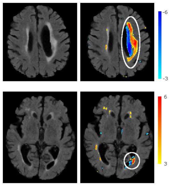
Figure 11 shows segmented abnormalities on a test sample with cortical infarcts and periventricular lesions. Thresholded abnormality maps are overlaid on the original FLAIR image for the visualization of segmented abnormalities on the image. We observe that the method successfully segments both types of pathology.

Figure 11.

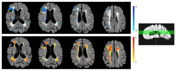
Segmentation of abnormalities on a sample image with cortical infarcts and periventricular lesions. Positive (red) and negative (blue) normalized abnormality maps overlaid on the image. Positive abnormality map is thresholded at t ≥ 3.1 (calculated through cross-validation), and negative map at t ≥ 3.5

Segmentation of white matter lesions

We evaluated the performance of our method on WML segmentation by comparing it to a voxel-based morphometry approach (Ashburner and Friston, 2000), where a voxelwise one-sample t-test method is applied. At each voxel, a t-statistic that measures the statistical significance of the test voxel’s intensity difference from the intensity distribution of the normal population is derived. An abnormality map is calculated for each test image.

Manual WML masks have been drawn by a radiologist on Set1, and by two raters trained by a radiologist on Set2. For both methods, preprocessed images of 21 subjects from both data sets with a lesion load higher than 10 cc³ are used as the test data. The segmentation accuracy is quantitatively measured by comparing the segmented WMLs to manual masks considered as gold standard. Also the inter-rater agreement is calculated for Set2. As the number of negative samples is much larger than the number of positive samples for the whole brain, Dice coefficient, which disregards the true negatives (TN), is used as a validation metric of the agreement. Dice coefficient measures the spatial overlap between two segmentations, and is defined as:

$$\mathit{DSc}(P_1,P_2)=\frac{2\times (P_1\cap P_2)}{P_1\cup P_2}$$ (14)

where P₁ and P₂ are the positive (e.g. lesion) voxels from the two segmentations.

The optimal threshold value for creating a binary mask from the abnormality map is calculated through cross validation using leave-one-out within each test data set. The threshold value that gives the maximum Dice coefficient is calculated for all test samples except the left-out sample. The average of these threshold values is used for thresholding the left-out subject. Sensitivity and specificity values are also calculated for the segmentation obtained using the selected threshold value.

Table 1 shows the average Dice coefficient, sensitivity and specificity values obtained for the lesion segmentation on both datasets compared to manual raters. Our method obtained Dice scores higher than the VBM method’s on all sets, and higher sensitivity on Set1 and on Set2 for the comparison with the first rater. The individual Dice coefficients obtained by each test sample are given in figure 12. We performed a two sided paired ttest on the results of our method and of the VBM approach. The differences between the two methods were significant (p = 0.0054 for masks from R1, p = 8.8 × 10⁻⁴ for masks from R2)

Table 1.

Quantitative comparison of segmentations using the proposed method (M1) and the VBM approach (M2) vs manual rater’s segmentations (Raters R1 and R2). Average values of Dice coefficient (DSc), specificity (Spec) and sensitivity (Sen).

		DSc	Sen	Spec
Set1	M1-R1	0.5382	0.4900	0.9997
	M2-R1	0.5343	0.4675	0.9997
Set2	M1-R1	0.6030	0.5608	0.9992
	M2-R1	0.5775	0.5302	0.9991
	M1-R2	0.6642	0.6129	0.9992
	M2-R2	0.6381	0.6247	0.9990

Figure 12.

Dice scores that measure the agreement, i.e. the amount of overlap, between different pairs of WML masks for each test image are shown. Two automatic segmentation methods, ours (M1) and the VBM (M2) were applied for each test image. For images in dataset Set1 a manual segmentation mask by only one rater (R1) was available. The Dice score is calculated betweeen each automated method and the manual segmentation. For images in dataset Set2 manual masks from two raters (R1,R2) were available. The Dice score is calculated between each automated mask and manual mask, as well as between the two manual masks to measure the inter-rater agreement.

Segmentation of cortical infarcts

Cortical infarcts are manually detected on Set2 by two independent raters, and their necrotic parts are segmented. The two raters independently detected the same 5 infarcts on 47 test images.

Accurate segmentation of the necrotic part of cortical infarcts is difficult even for manual raters, as the necrosis is often connected to adjacent sulci with similar intensity profile. Also, from a clinical perspective, rather than an exact segmentation, detecting the count, size and location of the infarcts is more important. For this reason, instead of calculating the Dice score that quantifies the overlap between two segmentations, we used the detection accuracy as our validation metric.

The method is applied first to compute normalized positive and negative abnormality maps. These maps are thresholded to segment hyper and hypo-intense abnormalities. Segmented hypo-intense voxels are clustered in 3-D clusters by applying a connected components algorithm, as candidates of necrosis. Clusters with a volume smaller than a threshold s_min are eliminated. A cluster is then classified as an infarct if the volume of hyperintense voxels around it in a predefined neighbourhood is higher than 50 % of the cluster volume. The neighbourhood volume, which varies linearly with the volume of the cluster, is calculated through the application of morphological dilation operations.

A cluster classified as an infarct is compared to ground-truth mask, and it is considered as a correct detection if the voxels within the cluster partially overlapped with necrosis segmented by both manual raters.

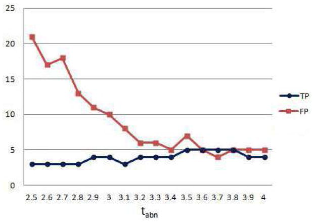
The classification algorithm is first applied for s_min = 20mm³, and a range of threshold values t_abn ∈ {2.5, …, 4} used for thresholding the negative abnormality map. The number of true positives (TP) and false positives (FP) are given in figure 13. The method reaches a 100 % sensitivity, i.e. detects all 5 infarcts correctly, when t_abn takes values between 3.5 and 3.8, with a low number of false positives in this range.

Figure 13.

Classification of infarcts. Number of true and false positives for different values of abnormality threshold for segmenting necrosis.

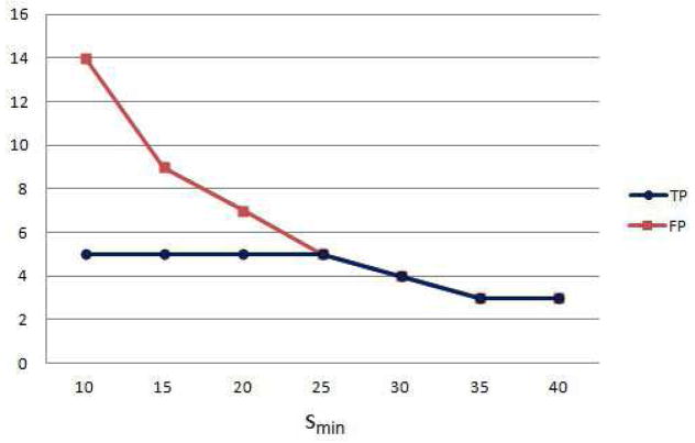
We investigated the effect of the cluster volume threshold on the classification accuracy, by applying the classification for t_abn = 3.5 and s_min ∈ {5, …, 40}. The results show that the number of false positives decreases for larger s_min, but some of the infarcts could not be detected when the volume threshold is too high (s_min > 25) (Figure 14).

Figure 14.

Classification of infarcts. Number of true and false positives for different values of minimum necrotic volume threshold.

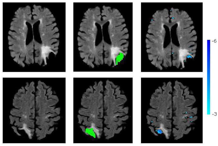
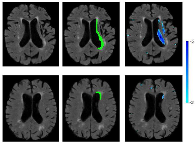
Figure 15 shows the segmentation of the necrotic parts of two cortical infarcts by the method, together with the manual segmentations. A visual qualitative analysis is performed to evaluate the segmentation accuracy and to understand the reasons of misdetections. We observed that due to lack of clear boundaries that separate necrosis from the CSF in normal sulci, the manual segmentation of the necrosis had a high inter-rater variability. Consequently, the overlap between automatically and manually segmented necrosis might be low, which results in false negatives. We also observed that false positives that persisted even for high s_min and t_abn values were mainly due to periventricular atrophy and posterior horn of the lateral ventricle, both misclassified as infarcts. Fig 16 shows two such misclassification cases.

Figure 15.

Segmentation of cortical necrosis. Left: FL image; Middle: Manual necrosis mask; Right: Necrosis segmented by the method.

Figure 16.

Sample cases of misclassifications: ventricular atrophy classified as infarct top), posterior horn of the lateral ventricle classified as infarct (bottom). Thresholded positive (red) and negative (blue) abnormality maps are overlaid on the FLAIR image.

Segmentation of periventricular atrophy

We analysed how sensitive the method was to abnormalities in size and shape of ventricles. A radiologist drew rough abnormality masks for ventricles for a subset of Set2 images. We visually compared the thresholded abnormality maps calculated by our method with these manual masks. Generally, the model captured regular enlargement of the whole ventricles as normal variation of the anatomy. As the training set belongs to an ageing population, the enlargement of the ventricles due to atrophy was observed in the training set, and should have been learned by the model as normal. Interestingly, significant partial deviations from normal, which can be visually recognized from the differences in the symmetry of left and right ventricles, were detected by the method as abnormal. These detections complied with the manual raters’ abnormality masks. One of these cases is shown in the top row of Figure. 16. Figure 17 shows two other cases.

Figure 17.

Segmentation of abnormal periventricular atrophy. Left: FL image; Middle: Atrophy mask drawn by a radiologist; Right: Atrophy segmented by the method.

4. Discussion and conclusion

We presented a generic framework for capturing statistical variations of imaging characteristics from a normative set of medical images (brain scans in these experiments), and for segmenting abnormalities as deviations from normality. Due to the challenge of high dimensionality of the image domain relative to the typically available sample sizes, we introduced an iterative strategy for sampling subspaces, estimating the pdf of each subspace, and projecting a test sample to the normal space as defined by each subspace model. A target-specific feature selection is further used to focus the pdf estimation only on the features of interest for a particular test subject, further alleviating the high-dimensionality problem. The difference between the test image and its projection to normal space highlights abnormalities. Cross-validation was used to estimate statistical significance of the voxelwise distances.

A linear model is used to estimate pdf s within subspaces. Approaches like Kernel PCA (Schlkopf et al., 1999) or Isomap (Tenenbaum et al., 2000) might be investigated in order to capture non-linearities in data and to learn the manifold structure of the normal anatomy within a subspace. However, two main challenges for the application of these approaches to our problem are 1) the requirement of a large number of training samples for a robust estimation of the underlying manifold structure of the normal brain anatomy, and 2) the difficulties of properly projecting a test sample into the estimated manifold of normal brains.

We used a weighted random selection strategy for sampling image subspaces. This approach currently has two limitations. First, the weights are initialized uniformly and updated based on the selection frequency, for providing an even sampling of image voxels. A possible modification would be an adaptive strategy, such that regions that are more likely to be abnormal will be more densely sampled. At each iteration, a global abnormality score can be calculated for the selected image patch, and the weights of voxels within this image patch can be updated accordingly. Alternatively, if prior knowledge exists on spatial locations of possible abnormality, this can be incorporated into the initial weights assigned to voxels. Second, only marginal pdf ’s of regional patches are currently estimated in this iterative procedure. More complex patterns can be missed this way, e.g. left/right hemispheric differences. Joint statistics of multiple patches, or else other methods for evaluating more complex spatial patterns, can be pursued in the future.

The training set that we used in our experiments contained a relatively small number of images. Construction of larger training sets would make the method more accurate, as the estimability of subspaces would increase with more training samples. Also, the average age of the training subjects was high. We observed that brain changes due to normal aging may be a confounding factor to brain changes due to pathologies. For example, parts of periventricular lesions on some of the test images were segmented as normal. That was most probably due to the prevalence of periventricular hyperintensities in training images. Periventricular white matter changes due to normal aging that is not associated with a disease process were reported in several MRI studies (Meguro et al., 1992; Ylikoski et al., 1995).

The method is applied for segmenting two common types of brain abnormalities with different characteristics. Thresholding and fuzzy clustering based techniques were widely used for automatic segmentation of WMLs (Admiraal-Behloul et al., 2005; Jackand et al., 2001). More recently, supervised learning methods obtained promising segmentation results (Anbeek et al., 2004; Lao et al., 2008). However, these methods mostly train on a specific type of abnormality, and thus their motivation is fundamentally different from the one that we presented in this paper. Segmentation of necrotic infarcts is known to be a more difficult problem due to the intensity overlap between the necrosis and the CSF. Automated methods that only rely on signal intensity generally fail in detecting them, while methods based on single atlas reported high false positive rates in the cortical regions (Shen et al., 2008).

Certain limitations of the proposed approach should be acknowledged. Most importantly, as the method aims to detect “all types of abnormalities”, it’s not expected to achieve the performance of dedicated, state-of-the art methods that specialize on segmenting a specific type of abnormality. Furthermore, generally being trained on features extracted from both normal and abnormal regions, such methods have a higher discriminatory power. Another limitation, related to the aforementioned one, is the lack of ground-truth data, which makes a quantitative evaluation of our method on less specific abnormalities difficult. Also, instead of adopting a purely discriminative approach, we aimed to create the image of the expected normal appearance from an image with abnormalities. The reconstruction of the normal anatomy has its own difficulties, mainly considering the very high dimensionality of the data and the high variation of healthy brain anatomy. We were only partially successful in capturing the cortical variation using the limited sample size available for training. In future, by incorporating many more images from healthy subjects into the model, the performance of our method could be improved.

The abnormality maps generated by applying our method could be used for various purposes: They can provide prior probabilistic maps for other methods that focus on detecting specific types of abnormalities. Such prior maps might increase the accuracy of these methods, and also decrease their computational complexity by reducing the dimensionality of the search space, for example by limiting the number of candidate regions before applying a specialized segmentation algorithm. Alternatively, a binary segmentation mask might be obtained by thresholding the abnormality map in different operational values, as we did in our experiments. The maps can be fed as input to population-based pattern analysis methods that aim to detect imaging patterns that differentiate groups of subjects, e.g. diseased and normal. Finally, a global abnormality score that will be calculated from each abnormality map might be used for early detection of subjects that require immediate attention of radiologists.

Highlights.

• We present a multi-variate pattern analysis method for segmenting abnormalities.

• The method aims to estimate the normal variation of the healthy anatomy;

• And to segment abnormalities as deviations from the estimated normal.

• An iterative sampling strategy is used to overcome the small sample size limitation.

• A target specific feature selection is applied to further reduce the dimensionality.

References

- Ashburner J, Friston KJ. Voxel-based morphometry–The methods. Neuroimage. 2000;11:805–821. doi: 10.1006/nimg.2000.0582. [DOI] [PubMed] [Google Scholar]
- Mechelli A, Price C, Friston K, Ashburner J. Voxel-Based Morphometry of the Human Brain: Methods and Applications. Current Medical Imaging Reviews. 2005:105–113. [Google Scholar]
- Burges CJC. A Tutorial on Support Vector Machines for Pattern Recognition. Data Min Knowl Discov. 1998;2(2):121–167. doi: http://dx.doi.org/10.1023/A:1009715923555. [Google Scholar]
- Cortes C, Vapnik V. Support-Vector Networks. Machine Learning. 1995;20:273–297. [Google Scholar]
- Anbeek P, Vincken K, van Osch M, Bisschops R, van der Grond J. Probabilistic Segmentation of White Matter Lesions in MR Imaging. NeuroImage. 2004;21(3):1037–1044. doi: 10.1016/j.neuroimage.2003.10.012. [DOI] [PubMed] [Google Scholar]
- Lao Z, Shen D, Liu D, Jawad AF, Melhem ER, Launer LJ, Bryan RN, Davatzikos C. Computer-Assisted Segmentation of White Matter Lesions in 3D MR Images Using Support Vector Machine. Academic Radiology. 2008;15(3):300–313. doi: 10.1016/j.acra.2007.10.012. [DOI] [PMC free article] [PubMed] [Google Scholar]
- Prastawa M, Bullitt E, Ho S, Gerig G. A brain tumor segmentation framework based on outlier detection. NeuroImage. 2004;21(3):1037–1044. doi: 10.1016/j.media.2004.06.007. [DOI] [PubMed] [Google Scholar]
- Shiee N, Bazin PL, Ozturk A, Reich D, Calabresi P, Pham D. A topology-preserving approach to the segmentation of brain images with multiple sclerosis lesions. Neuroimage. 2010;49(2):1524–35. doi: 10.1016/j.neuroimage.2009.09.005. [DOI] [PMC free article] [PubMed] [Google Scholar]
- Van Leemput K, Maes F, Vandermeulen D, Suetens CAP. Automated segmentation of multiple sclerosis lesions by model outlier detection. IEEE Transactions on Medical Imaging. 2001;20(8):677–688. doi: 10.1109/42.938237. [DOI] [PubMed] [Google Scholar]
- Wu Y, Warfield S, Tan I, Wells W, Meier D, van Schijndel R, Barkhof F, Guttmann C. Automated Segmentation of Multiple Sclerosis Lesion Subtypes with Multichannel MRI. Neuroimage. 2006;32(3):1205–1215. doi: 10.1016/j.neuroimage.2006.04.211. [DOI] [PubMed] [Google Scholar]
- Erus G, Zacharaki E, Bryan N, Davatzikos C. Learning high-dimensional image statistics for abnormality detection on medical images. MMBIA 2010: IEEE Computer Society Workshop on Mathematical Methods in Biomedical Image Analysis; San Francisco, CA, USA. 2010. [Google Scholar]
- Donoho DL. De-noising by soft-thresholding. IEEE Transactions on Information Theory. 1995;41(3):613–627. [Google Scholar]
- Sjostrand K, Rostrup E, Ryberg C, Larsen R, Studholme C, Baezner H, Ferro J, Fazekas F, Pantoni L, Inzitari D, Waldemar G. Sparse Decomposition and Modeling of Anatomical Shape Variation, Medical Imaging. IEEE Transactions on. 2007;26(12):1625–1635. doi: 10.1109/tmi.2007.898808. [DOI] [PubMed] [Google Scholar]
- Barkhof F. Guidelines for brain imaging in vascular dementia clinical trials. Int Psychogeriatry. 2003;15:273–6. doi: 10.1017/S1041610203009323. [DOI] [PubMed] [Google Scholar]
- Roweis ST, Saul LK. Nonlinear dimensionality reduction by locally linear embedding. SCIENCE. 2000;290:2323–2326. doi: 10.1126/science.290.5500.2323. [DOI] [PubMed] [Google Scholar]
- Tenenbaum JB, Silva V, Langford JC. A Global Geometric Framework for Nonlinear Dimensionality Reduction. Science. 2000;290(5500):2319–2323. doi: 10.1126/science.290.5500.2319. [DOI] [PubMed] [Google Scholar]
- Gerber S, Tasdizen T, Fletcher P, Joshi S, Whitaker R. the Alzheimers Disease Neuroimaging Initiative (ADNI), Manifold modeling for brain population analysis. Medical Image Analysis. 2010;14(5):643–653. doi: 10.1016/j.media.2010.05.008. [DOI] [PMC free article] [PubMed] [Google Scholar]
- Hamm J, Verma DYR, Davatzikos C. Gram: A framework for geodesic registration on anatomical manifolds. Medical Image Analysis. 14(5) doi: 10.1016/j.media.2010.06.001. [DOI] [PMC free article] [PubMed] [Google Scholar]
- Zacharaki EI, Bezerianos A. Abnormality segmentation in brain images via distributed estimation. IEEE Trans Inf Technol Biomed. doi: 10.1109/TITB.2011.2178422. [DOI] [PubMed] [Google Scholar]
- Canny J. A computational approach to edge detection. IEEE Trans Pattern Anal Mach Intell. 1986;8:679–698. [PubMed] [Google Scholar]
- Mallat S, Wavelet A. Tour of Signal Processing, Third Edition: The Sparse Way. 3. Academic Press; 2008. [Google Scholar]
- Smith S. Fast robust automated brain extraction. Human Brain Mapping. 2002;17:143–155. doi: 10.1002/hbm.10062. [DOI] [PMC free article] [PubMed] [Google Scholar]
- Sled J, Zijdenbos A, Evans A. A nonparametric method for automatic correction of intensity nonuniformity in MRI data. IEEE Trans Med Imaging. 1998;17:87–97. doi: 10.1109/42.668698. [DOI] [PubMed] [Google Scholar]
- Shen D, Davatzikos C. HAMMER: Hierarchical attribute matching mechanism for elastic registration. IEEE Trans Med Imaging. 2002;21:1421–1439. doi: 10.1109/TMI.2002.803111. [DOI] [PubMed] [Google Scholar]
- Schlkopf B, Smola AJ, Müller KR. Kernel principal component analysis. Advances in kernel methods: support vector learning. 1999:327–352. [Google Scholar]
- Meguro K, Sekita Y, Yamaguchi T, Yamada K, Hishinuma T, Matsuzawa T. A study of periventricular hyperintensity in normal brain aging. Archives of Gerontology and Geriatrics. 1992;14(2):183–191. doi: 10.1016/0167-4943(92)90053-7. [DOI] [PubMed] [Google Scholar]
- Ylikoski A, Erkinjuntti T, Raininko R, Sarna S, Sulkava R, Tilvis R. White matter hyperintensities on MRI in the neurologically nondiseased elderly. Analysis of cohorts of consecutive subjects aged 55 to 85 years living at home. Stroke. 1995;26:1171–1177. doi: 10.1161/01.str.26.7.1171. [DOI] [PubMed] [Google Scholar]
- Admiraal-Behloul F, van den Heuvel DMJ, Olofsen H, van Osch MJP, van der Grond J, van Buchem MA, Reiber JHC. Fully automatic segmentation of white matter hyperintensities in MR images of the elderly. Neuroimage. 2005;28(3):607–17. doi: 10.1016/j.neuroimage.2005.06.061. [DOI] [PubMed] [Google Scholar]
- Jackand CR, O’Brien PC, Rettman DW, Shiung M, Xu Y, Muthupillai R, Manduca A, Avula R, Erickson BJ. FLAIR histogram segmentation for measurement of leukoaraiosis volume. J Magn Reson Imaging. 2001;14(6):668–76. doi: 10.1002/jmri.10011. [DOI] [PMC free article] [PubMed] [Google Scholar]
- Shen S, Szameitat AJ, Sterr A. Detection of infarct lesions from single MRI modality using inconsistency between voxel intensity and spatial location–a 3-D automatic approach. IEEE Trans Inf Technol Biomed. 12(4) doi: 10.1109/TITB.2007.911310. [DOI] [PubMed] [Google Scholar]