Complex role of space in the crossing of fitness valleys by asexual populations

Abstract

The evolution of complex traits requires the accumulation of multiple mutations, which can be disadvantageous, neutral or advantageous relative to the wild-type. We study two spatial (two-dimensional) models of fitness valley crossing (the constant-population Moran process and the non-constant-population contact process), varying the number of loci involved and the degree of mixing. We find that spatial interactions accelerate the crossing of fitness valleys in the Moran process in the context of neutral and disadvantageous intermediate mutants because of the formation of mutant islands that increase the lifespan of mutant lineages. By contrast, in the contact process, spatial structure can accelerate or delay the emergence of the complex trait, and there can even be an optimal degree of mixing that maximizes the rate of evolution. For advantageous intermediate mutants, spatial interactions always delay the evolution of complex traits, in both the Moran and contact processes. The role of the mutant islands here is the opposite: instead of protecting, they constrict the growth of mutants. We conclude that the laws of population growth can be crucial for the effect of spatial interactions on the rate of evolution, and we relate the two processes explored here to different biological situations.

1. Introduction

Complex traits can depend on the interactions between several different genetic loci [1]. In this context, the evolution of advantageous phenotypes can require the accumulation of several mutations within one individual. Each of these mutations is usually assumed to be neutral or deleterious (but in general can also be assumed to be slightly advantageous). Therefore, in order to attain the advantageous type, evolution has to cross a fitness plateau if the partial mutants are neutral compared with the wild-type, a fitness valley if they are deleterious [1–3] or a ‘fitness foothill’ if the intermediate mutants are slightly advantageous. This can apply to several biological situations, a few examples of which are as follows. Biological activity often requires the interactions between different proteins within cells, and the availability of only a subset of the components either does not lead to a fitness advantage or results in a fitness disadvantage. Well-known examples are signalling mechanisms that regulate cell proliferation and differentiation [4]. Another example is the aberrant growth of cancer cells, which can require multiple mutational hits [5], each of which can be neutral or disadvantageous compared with healthy cells in the tissue. The escape of pathogens from immune responses within hosts can incur fitness costs [6,7], and an advantage can only be achieved once the pathogen has escaped a number of different immune responses that simultaneously attack the infectious agent [8]. Communities of microorganisms, such as biofilms, build support structures that can be dependent on the interactions between different gene products [9].

Scenarios where intermediate mutants are slightly advantageous compared with the wild-type, and the complex trait is even more advantageous (evolutionary foothills), are also common in nature. An interesting example is the evolution of p53 loss, leading to accelerated and uncontrolled cell growth and the formation of tumours [10]. While complete loss of p53 function has been mainly attributed to an inactivation of both copies of the gene, a dominant negative effect has also been documented, in which a single mutated copy of the gene can reduce overall p53 function to a certain degree through disruption of p53 tetramer formation, which is required for function [10].

The accumulation of multiple mutations within an individual required to attain a fitness advantage can be a long process, and understanding the rate at which fitness plateaus/valleys/foothills are crossed is important for determining the feasibility of specific evolutionary processes within realistic time frames. While recombination can bring together multiple mutations within an organism [11], evolution in asexual populations strictly depends on the sequential accumulation of mutations within a lineage. This can occur by two basic mechanisms [3]. (i) Sequential fixation is a series of transitions where consecutive intermediate mutants (with 1, 2, etc., sites mutated) become fixated in the population, until the final, advantageous phenotype is finally generated. (ii) Stochastic tunnelling [12,13] is the creation of an advantageous trait without a prior fixation of intermediate mutants. In this process, intermediate mutants exist transiently at relatively low numbers, and the advantageous type is created in their midst. If more than two mutations need to be accumulated to gain a fitness advantage, then a combination of these processes can also occur which includes fixation of some intermediate mutants, and a tunnelling process that skips the fixation of the rest of the mutational steps.

The rate at which the fitness valley is crossed, and thus the time until the advantageous phenotype emerges, has been analysed mathematically for different assumptions [2,3,12–21]. The rate of tunnelling was first calculated in [12] and then in [13]. A very detailed theory of fitness valley crossing by asexual populations is presented in [3]. In all these papers, the assumption of mean-field or mass action was used where the spatial locations of individuals were not taken into account. In this paper, we ask how spatial interactions might change the dynamics of fitness valley crossing.

The first spatial generalization of this problem was studied theoretically in [22], where a one-dimensional spatial Moran process was considered. It was found that the rate of tunnelling is higher in the model with nearest-neighbour interactions, compared with the mass-action model. Similar results were found for two- and three-dimensional models [20,21], and the effect of migration on these evolutionary processes was studied in [23]. All of this work considered Moran processes, which are birth–death processes in a constant population. In particular, these models assume that the death of an individual is immediately balanced by the birth of another, thus not allowing for variation in the population size or for empty space. In addition, these models were studied in the context of two sites that need to be mutated in order to attain the advantageous trait, and only the situation of the nearest-neighbour interactions was considered.

This paper explores the role of spatial interactions for the rate at which fitness valleys are crossed more generally, comparing different population growth processes in two dimensions. In addition to the Moran process, we also consider a different type of model, called the contact process, where the population size is determined by the birth and death rates and where it is possible to have empty, unoccupied space. This relaxes the very rigid requirement of a microscopic balance between births and deaths in the Moran model. The Moran process can be considered as a limiting case of the contact process where the division rates are extremely high compared with death rates. In this paper, we examine the dynamics for different numbers of sites that need to be mutated to attain the advantageous phenotype, and explore the whole range of spatial restriction, from the nearest-neighbour model to the mass-action (homogeneously mixing) scenario. We examine the cases of disadvantageous, neutral and advantageous intermediate mutations.

It turns out that the effects of spatial structure on the rate of evolution in these models are not straightforward.

• — In the Moran process, spatial interactions speed up the evolution of the complex trait for neutral and disadvantageous intermediate mutants, consistent with previous work [20–22].

• — For advantageous intermediate mutants in the Moran process, spatial interactions slow down the evolution of the complex trait. This is the opposite effect of space compared with the case of neutral and disadvantageous intermediate mutants.

• — In the contact process for neutral and disadvantageous intermediate mutants, spatial interactions can either accelerate or slow down the rate of evolution, depending on the mutation rate. It is also possible to have an intermediate optimal interaction radius (between mass-action and nearest-neighbour interactions), which minimizes the time until the advantageous trait emerges.

• — For advantageous intermediate mutants in the contact process, spatial interactions speed up the evolution of the complex trait, even more so than in the Moran process.

The two types of models (the Moran and the contact processes) correspond to different biological scenarios, which we discuss.

2. The Moran (constant population) process

We first consider the Moran process, as this allows a greater degree of mathematical insight. We will restrict our attention to a process in a two-dimensional square grid of size N, with periodic boundary conditions. In this process, individuals die at random, independently of their phenotype, and are immediately replaced by the progeny of one of the nearby individuals, selected randomly from the square neighbourhood of a fixed size, M. The probability to be selected for reproduction is proportional to the fitness of each phenotype, and mutations happen with a given probability for each out of m sites upon reproduction. Back-mutations are not taken into account. Figure 1a shows an example of a mutation diagram for m = 3 sites. The population size stays constant (equal to N) after each update, and there are no empty spots on the grid.

Figure 1.

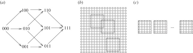
The simulation set-up. (a) The combinatorial mutation diagram for m = 3 sites. (b) The concept of neighbourhood, illustrated with the neighbourhoods of radius 2. (c) The patch model: the population is split into n patches. At each update, an individual is removed at random from a random patch, and is replaced by an offspring of another individual, chosen from the same patch according it its fitness.

We investigate the role of spatial interactions by varying the neighbourhood size where the individuals can place their offspring. If, for a given individual, the neighbourhood only includes the eight surrounding spots on the square grid, this corresponds to the nearest-neighbour situation, or a ‘radius 1 neighbourhood’. If the neighbourhood is as big as the whole population, then this is a mass-action (homogeneously mixing) system. An example of a neighbourhood of radius 2 is shown in figure 1b. The question we ask is how the rate of m-hit mutant production depends on the neighbourhood size.

2.1. Spatial structure accelerates evolution

Numerical simulations of this process are presented in figure 2, assuming that two loci need to be mutated to acquire the advantageous phenotypes (m = 2). There, for each neighbourhood size, we ran the process at least 10⁵ times, stopping when the m-hit mutant was generated, and recording the waiting times. An example of mean waiting times as a function of the neighbourhood radius is shown in figure 2a. The exact distribution of waiting times for different neighbourhood sizes is shown in the form of histograms in figure 2b,c. We can see that, even if the differences in the mean waiting times between the homogeneously mixing and the nearest-neighbour model are smaller than the widths of the distributions, these distributions are clearly distinct, and the means are significantly different (with the p-value in both the t-test and Mann–Whitney U-test less than 10⁻¹⁰). In fact, for the examples presented in figure 2b,c, the sample size of only 2500 and 1000 points, respectively, consistently yields p-values smaller than 0.05 for the Mann–Whitney U-test.

Figure 2.

Effect of the neighbourhood radius on the time at which the m-hit mutant arises in the Moran process. (a) The average time of emergence for four neighbourhood radii: 1, 2, 10 and 50. Averages are based on at least 10⁵ iterations of the simulation. The chosen parameters were: grid size N = 50 × 50, m = 2, intermediate mutants were neutral, u = 10⁻⁴. (b) Histograms showing the distribution of outcomes, corresponding to the data presented in part (a). For the sake of simplicity, only two radii are compared: 1 and 50. (c) Same type of histogram, but with u = 10⁻⁵, showing a greater difference. (Online version in colour.)

We observe (figure 2a) that the waiting times increase monotonically with the neighbourhood size. We can see that the waiting times reach saturation and stop changing after the neighbourhood size reaches a certain value (of the order M ∼ NlnN^−1/2 [24]), where the system is effectively mass action. On the other hand, tight spatial interactions (small values of M) lead to a faster m-hit mutant production. The results hold for both neutral and disadvantageous intermediate mutants. An intuitive explanation for this phenomenon that was proposed in [22] evokes the concept of mutant islands. Under mass-action rules, all types are mixed randomly (figure 3a). On the other hand, if reproduction is allowed only within a small neighbourhood, then spatial structures tend to form, where the nearby individuals are likely to have identical genotypes (figure 3b). For example, in the case of m = 2, where one-hit mutants are neutral or disadvantageous, once a one-hit mutant is generated, its clone (if it has a chance to form) will be located in the vicinity of the original de novo mutation. It can be argued that such localized clones are, on average, longer-lived than spatially dispersed clones. This is because a dead mutant is more likely to be replaced by the progeny of another mutant than a wild-type individual, if most of its neighbours are mutants. In turn, longer-lived clones of intermediate mutants are more likely to produce m-hit mutants, which speeds up the process of m-hit mutant generation.

Figure 3.

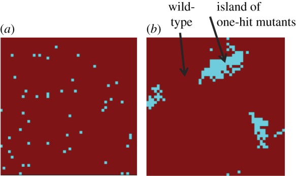
Spatial configuration of the Moran process for the case of (a) mass action and (b) a neighbourhood radius of 1. In the presence of spatial structure, islands of intermediate mutants are observed. The chosen parameters were: grid size = 50, m = 2, intermediate mutants were neutral, u = 10⁻⁴. (Online version in colour.)

How tight the mutant islands are depends on the neighbourhood size. For very small neighbourhoods, the dynamics are the most localized, and the islands are more pronounced than in systems with larger neighbourhood sizes.

Note that our results do not depend on the particular grid sizes chosen. Grid sizes that are significantly larger than those chosen in our illustrations are computationally very costly. In the electronic supplementary material (section 4), we show that the same trends are observed in a 200 × 200 grid as in a 50 × 50 grid.

2.2. Dependence on parameters

The extent to which spatial structure accelerates the emergence of the m-hit mutant depends on parameters. In particular, it depends on the mutation rate, because this parameter influences the importance of mutant islands for the emergence of the complex phenotype. Figure 4 shows the relative mean waiting time for the homogeneously mixing system compared with that for the nearest-neighbour system, for different mutation rates. For each mutation rate, we calculated the mean waiting time for the m-hit mutants in the mass-action model, and divided it by the mean waiting time in the nearest-neighbour setting. This ratio was plotted for several different values of the mutation rate, u. Figure 4a,c,e corresponds to neutral intermediate mutants, and figure 4b,d to disadvantageous mutants. We can see a common pattern, where, for very high mutation rates, the spatial interactions do not have much influence on the rate of m-hit mutant generation (the ratio of waiting times is close to 1). For intermediate mutation rates, the spatially restricted systems produce mutants significantly faster (the ratio greater than 1). Then, for low mutation rates, the difference between spatial and non-spatial systems either stops changing with u (for disadvantageous intermediate mutants) or it decreases (for neutral intermediate mutants).

Figure 4.

Time to emergence of m-hit mutant in the Moran process. Compared are mass action relative to extreme spatial restriction, where the neighbourhood radius is 1. The time to emergence for radius = 1 was set to unity, and the time observed for mass action was scaled accordingly. This number is plotted against the mutation rate, u. (a) m = 2, grid size N = 10 × 10, neutral intermediate mutants. (b) m = 2, N = 10 × 10, intermediate mutants have 10% fitness cost. (c) m = 2, N = 50 × 50, neutral intermediate mutants. (d) m = 2, N = 50 × 50, intermediate mutants have 10% fitness cost. (e) m = 4, N = 50 × 50, neutral intermediate mutants.

As is clear from this summary, the mutation rate is a crucial parameter that dictates the behaviour of the system. In the following, we describe in detail and explain the dynamics in the different regimes, i.e. for high, intermediate and low mutation rates. These categories are defined relative to other parameters, as explained below. The boundaries separating the categories are calculated analytically, and these calculations are illustrated by numerical examples.

(i). High mutation rates

For relatively large mutation rates, the difference between the spatial and mass-action systems is very small. This is because, for very high mutation rates, new mutants are produced very frequently, and are accumulated mostly by de novo production rather than by mutant reproduction (this regime corresponds to neutral semi-deterministic tunnels of [3]). In this case, the role of mutant islands is negligible, and the waiting time is not changed by the neighbourhood size. Figure 5a shows a typical time series of mutant generation for high mutation rates. We can see that intermediate mutants are generated constantly and experience a steady climb. This behaviour is similar to the behaviour of advantageous mutants. The presence of a one-way mutation process at a high rate effectively makes neutral mutants behave like advantageous mutants.

Figure 5.

Time-series simulation showing the evolutionary dynamics for (a–d) the Moran process and (e–h) the contact process, assuming m = 4, a 50 × 50 grid and neutral intermediate mutants. Wild-types are shown in black, intermediate one-, two- and three-hit mutants are shown in blue, green and pink, respectively. The advantageous four-hit mutant is shown in red. For the Moran process, the mutation rates were (a) u = 10⁻², (b) u = 10⁻³, (c) u = 10⁻⁴, (d) u = 10⁻⁵. For the contact process, L/D = 3, and (e) u = 10⁻², (f) u = 10⁻³, (g) u = 10⁻⁴ and (h) u = 10⁻⁵. The simulations were run under mass-action settings. (Online version in colour.)

This behaviour is observed if the mutation rate is significantly larger than a threshold, This threshold for the case of m = 2 can be determined from the work of [3,12]: for neutral intermediate mutants when 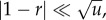and 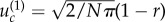for disadvantageous mutants.

To illustrate these formulae, we applied them to specific cases. For the parameter values in figure 4, we obtain for both neutral and disadvantageous cases with N = 10 × 10 (figure 4a,b), and it is and for neutral and disadvantageous cases, respectively, with N = 50 × 50 (figure 4c,d). We can see that the bounds obtained analytically indeed correspond to the change in the behaviour observed numerically.

(ii). Intermediate mutation rates

As the mutation rates become smaller than the accelerating role of space in m-hit mutant generation becomes more pronounced, because de novo mutant generation is less frequent now, and the mutant island effect becomes more important. Figure 5b,c shows typical time series in this regime, where the m-hit mutant is formed by stochastic tunnelling, with no intermediate mutants reaching fixation.

(iii). Low mutation rates

For even smaller values of u, there is another change in behaviour. This time the system behaves differently for neutral and disadvantageous intermediate mutants. These are considered in turn.

Neutral intermediate mutants. In the case of neutral intermediate mutants, when (which is defined later), the role of space is again diminished (figure 4a,e); figure 4c does not show this regime, because simulations for lower mutation rates for the given parameter values are exceedingly long. We can see that the difference between the spatial and non-spatial model for very low mutation rates is smaller than that for intermediate mutation rates. The explanation again is given by the time series (figure 5d). For very small mutation rates, sequential fixation takes place for one or more consecutive mutants. The reason is that it is unlikely to mutate the next locus before the preceding mutant has reached fixation. The total waiting time now consists of two parts: the time waiting for fixation (one or more) and the time waiting for tunnelling through the rest of the intermediate mutations. While the tunnelling rate is accelerated by spatial constraints, fixation events take somewhat longer in the nearest-neighbour model compared with mass action, simply because the spread of mutants happens via ‘surface growth’, where the expansion can take place only at the outside rim of the mutant island, compared with the bulk growth of the mass-action model. The two effects act in the opposite ways, and we can see that the mass-action waiting time for such small mutation rates is not too different from that of the nearest-neighbour model.

The threshold value is derived in the electronic supplementary material, section 1. In the symmetric case where all the mutation rates are the same and given by u, the expression for is given by In particular, for m = 2, we simply have For the parameters in figure 4, we have for N = 10 and m = 2 (figure 4a), for N = 50 and m = 2 (figure 4c) and for N = 50 and m = 4 (figure 4e). Again, we observe a good agreement of the analytical expressions and the observations.

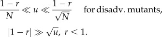
Disadvantageous intermediate mutants. In the case where r < 1 and fixation of intermediate mutants is very unlikely. There, the difference between spatial and non-spatial rates of m-hit mutant production does not decrease for small values of u, but it merely stops increasing. In other words, starting from some threshold value, decreasing u does not lead to further growth in the ratio of waiting times. This threshold value can be estimated if we impose the condition that the time scale of new mutant production (given by 1/(Nu)) is significantly larger than a typical lifespan of a disadvantageous mutant (given approximately by 1/(1 − r); see [11]). We then have the value 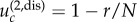, which corresponds to values 10⁻³ and 4 × 10⁻⁵ for N = 10 × 10 and N = 50 × 50 with r = 0.9, respectively; see figure 4b,d.

2.3. Summary of the mutation rate studies

As explained above, the range of mutation rates, u, splits into three qualitatively different regions, depending on whether spatial structures accelerate evolution. The boundaries between these regions are defined by particularly concise expressions for the Moran process in the case of m = 2. There, the range of mutation rates for which space accelerates evolution is given by

2.1

and

These three regions are similar to the three regimes in [25], where evolutionary mutant dynamics was studied in the context of two mutations leading to the inactivation of tumour suppressor genes in cancer. Small, intermediate and large populations were identified, which were characterized by different types of mutant dynamics. The population size was determined relative to the fixed mutation rates, and the bounds coincide with the ones in equation (2.1).

Our results are a particular example of the general notion that the evolutionary processes change qualitatively depending on the mutation rate (in relation to other parameters). For example, in [26,27], evolutionary games were studied in finite populations. For very small mutation rates, the dynamics can be approximated by a Markov chain on pure states; the smallness of u may differ depending on the game. In particular, for a coexistence game, where the best reply to any strategy is the opposite strategy, the threshold value of u is very small: 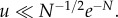Interestingly, for all other games, it is sufficient if the mutation satisfies 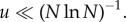The right inequality in equation (2.1) belongs to that category (but the condition is weaker because it is a necessary condition for a particular ‘game’).

2.4. Analogy with a patch model

In order to gain analytical insights into the spatially restricted models, we use an auxiliary system, which can help us quantify the idea of mutant island formation. From our study of the spatially restricted Moran process, we saw that the formation of clusters of intermediate mutants facilitates the generation of m-hit mutants, because tight clusters have a longer life expectancy than disperse sets of mutants. Let us take the idea of mutant islands to its extreme, and assume that the islands (of the size of the neighbourhood) cannot be invaded by the offspring of individuals from the outside. This brings us to the patch model, which is built by the fragmentation of the original Moran process.

Suppose that there are n separate patches of size M = N/n (figure 1c). As before, an individual is randomly removed (from a randomly chosen patch), and is replaced by the offspring of an individual in the same patch. As before, reproduction happens proportional to the individuals' fitness. In the case where n = 1 and M = N, this model is exactly identical to the mass-action Moran process. For n > 1, the patch model with patches of size M is used to inform us qualitatively about the behaviour of the Moran process with neighbourhood size M.

For such fragmented systems, we can calculate an approximation to the mean time of m-hit mutant generation in the case where m = 2; see the electronic supplementary material, section 2. For example, for neutral intermediate mutants, an explicit formula can be obtained and involves the hypergeometric function

2.3

where 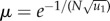, and we further denoted

2.4

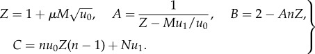
For neutral or disadvantageous intermediate mutants, the following approximations can be derived:

2.5

Here R₀ is the tunnelling rate starting from the population of wild-type individuals, is the fixation probability of one-hit mutants starting from M − 1 wild-type individuals and 1 one-hit mutant, and 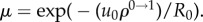We observe that, for both neutral and disadvantageous cases, equation (2.1) is an increasing function of the patch size M, and equation (2.2) the dependence of on M becomes negligible for large mutation rates The first of these observations corresponds to the role of patches (or mutant islands) in the creation of m-hit mutants, which was described above in the context of the Moran process. The second observation helps us explain why the role of space is negligible for high mutation rates, as described above.

3. The contact process

Next, we consider a model that is arguably more realistic than the Moran process described above. In the Moran process, each death is immediately followed by a reproduction event, which makes the model analytically tractable, but imposes a very rigid constraint on the timing of events. In what follows, we describe a model that is more widely used in ecological and evolutionary simulations, and which is a type of a contact process studied in different contexts [28].

In a square two-dimensional grid of size N, nodes can be unoccupied or occupied with cells of different types. Each time step consists of vN elementary updates, where v is the mean density of individuals and vN is the total number of occupied sites. At each elementary update, we pick an individual at random. With probability 0 < D < 1, this individual is removed, and with probability L = 1 − D, it attempts reproduction. Reproduction proceeds as follows. A random site in the neighbourhood of size M of this individual is picked, and, if it is occupied, the reproduction is aborted, and the update is complete. If the site is empty, the offspring (possibly with a mutation) of the individual is placed at the site, which completes the update. The Moran process, described earlier in this paper, can be considered the limit of the contact process where (except the time steps proceed uniformly in our version of the Moran process, and they happen with exponentially distributed time steps in this limit of the contact process). In the case where the grid is completely filled with live cells at all times, and the dynamics are driven by the death events, each of which is immediately followed by a division event.

Another connection of the contact process with the Moran process (under general values of L and D) is presented in the electronic supplementary material, section 3, where we show that the mass-action (M = N) version of the contact process can be expressed as a Moran process. The spatially restricted version of this model, however, exhibits somewhat different properties.

3.1. The steady-state density of cells

Before we explore the question of the rate of fitness valley crossing in the contact process, we need to gain an understanding of the model's basic properties. It turns out that the presence of unoccupied spots in the contact process leads to the formation of certain macroscopic structures, which in turn influence the course of evolutionary dynamics.

Let us set the mutation rates to zero and simply observe the spatio-temporal behaviour of individuals on the grid. Let us suppose that L > D. In the mass-action model, the process reaches a quasi-stationary state where the individuals are distributed around the grid with the equilibrium density of

3.1

(the subscript m.a. refers to ‘mass action’). That is, there are typically N(1 − D/L) individuals, they are distributed uniformly throughout the grid, with the probability of each site to be occupied given by ν_m.a.. This result can be derived very easily by assuming a uniform distribution of individuals and equating the probability of death with the probability of successful reproduction.

Things are significantly more complicated in a spatially restricted model (M < N). In this case, it is known that the probability of reproduction L has to be greater than a threshold value, L_c > D, for the system to reach the quasi-steady state, but the exact value of L_c is not theoretically known. Also, the equilibrium density has not been calculated (apart from the limiting values as M → N [24]). In the regime of interest, where no estimates of the equilibrium density are available.

The complication comes from the macroscopic structures forming in the system in the case of spatially restricted interactions (figure 6). In figure 7, we show numerically obtained steady-state numbers of individuals as a function of the neighbourhood size, M. We can see that the resulting density is lower than the mass-action density ν_m.a.. An attempt to describe this behaviour was made by the pair approximation method, which takes local interactions into account by considering pair correlations of neighbouring sites [29,30]. Unfortunately, this approximation crudely underestimates the difference between the spatial behaviour and the mass-action behaviour.

Figure 6.

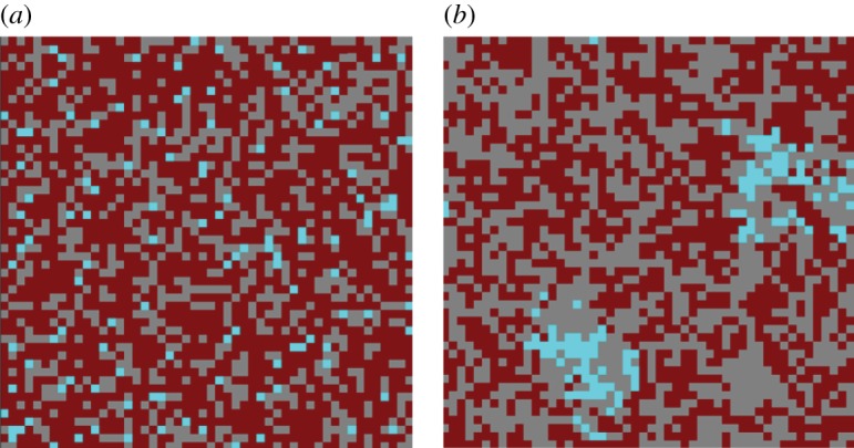
Spatial configuration of the contact process model for the case of (a) mass action and a neighbourhood radius of 1 (b). Grey depicts empty space. Wild-types are shown in dark (red), and one-hit mutants in light (cyan) colouring. In the presence of spatial structure, islands of intermediate mutants are observed. Individuals are not evenly distributed, but form macroscopic structures. The chosen parameters were: grid size 50 × 50, m = 2, intermediate mutants were neutral, u = 10⁻⁴, L/D = 3. (Online version in colour.)

Figure 7.

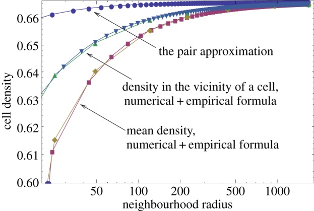
Numerically calculated densities of cells in the contact process, plotted as functions of the neighbourhood radius. We present the mean density (together with the empirical formula equation (3.2)), and the mean density of cells in a neighbourhood of non-empty spots (together with the empirical formula equation (3.3)). Also plotted is the pair approximation of the mean density. The parameters are N = 41 × 41, and L/D = 3. (Online version in colour.)

To capture the spatial effects more effectively, we studied the numerically generated quantity (1 − v)L/D as a function of the neighbourhood size, M. For the mass-action system, this quantity is simply 1. For the spatially structured system, this quantity grows as M decreases. We note that this quantity is very well described by a simple inverse function of M, which yielded the following empirical formula:

3.2

Here, the quantity c does not depend on M (but it appears to depend on the parameter D/L; for example, c ≈ 4 for D/L = 1/3 and c ≈ 4.5 for D/L = 1/2). This formula is demonstrated in figure 7, where it is plotted against simulations.

Next, we investigated the ‘local’ density of individuals, by measuring the number of occupied spots in the neighbourhood of each individual, averaged over all the individuals. This gave rise to an empirical formula for local density,

3.3

where c₁ and α do not depend on M (with c₁ ≈ 1.6 and α ≈ 0.9 both for D/L = 1/3 and D/L = 1/2). This formula is also demonstrated in figure 7, where it is plotted against simulations.

We observe the following two important trends:

• (1) The density in the vicinity of an occupied spot is greater than the mean density. The distribution of cells throughout the grid is no longer uniform, and the probability of finding an occupied site in the vicinity of a given individual is higher than the mean density. This is a quantification of the clustering effect, which can also be observed by simply examining a typical spatial distribution of individuals in a spatially structured system (figure 6b).

• (2) The mean number of individuals and the mean number of neighbours of an individual both increase with the neighbourhood size, M, and approach N(1 − D/L) as M → N (the mass-action limit). This can be viewed as a direct consequence of macroscopic structures. For smaller values of M, the density becomes non-uniform, with the local density higher than the average density. This makes individuals land on other occupied spots and thus reduces the number of successful events per time step. The number of successful divisions at equilibrium must be matched by the deaths, which are proportional to the total population. Therefore, the total population in spatial systems must be lowered compared with the mass-action system.

The importance of these trends for our evolutionary question becomes clear once we realize that the equilibrium number of individuals as well as the number of neighbours of a given individual define the time scale of the contact process. This is explained below, after we talk about the empirical observations for this model.

3.2. Complex effects of spatial structure

The effect of spatial structure on the waiting time for the emergence of the m-hit mutant is more complicated than that in the Moran process model. In the current setting, spatial structure can either accelerate or delay the generation of the m-hit mutant, depending on parameters. In some cases, there is an optimal neighbourhood size that maximizes the rate of emergence of the m-hit mutant. That is, evolution works fastest for intermediate-range interactions. Figure 8 presents some typical results. In figure 8, for a given mutation rate u, we calculated the mean waiting time for the m-hit mutant emergence for several neighbourhood radii, and divided it by the mean waiting time for the nearest-neighbour scenario (the radius 1 neighbourhood model). These relative mean waiting times were plotted as functions of the neighbourhood radius, for different mutation rates. In figure 8a and figure 8b, we have m = 2 and the intermediate mutants are neutral and disadvantageous, respectively. In figure 8c, we have m = 4 with neutral intermediate mutations. We can see that the waiting time decays monotonically with the neighbourhood radius, e.g. for u = 10⁻² in figure 8a,b and u = 10⁻³ in figure 8a. It increases monotonically for u = 10⁻⁵ in figure 8a,b and for u = 10⁻⁴ in figure 8b,c. The waiting time as a function of the neighbourhood radius experiences an intermediate minimum for u = 10⁻⁴ in figure 8a, for u = 10⁻³ in figure 8b,c, and for u = 10⁻² in figure 8c.

Figure 8.

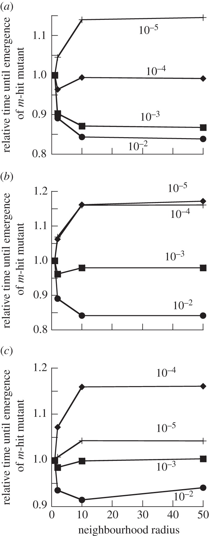
Time to emergence of m-hit mutant in the contact process. Compared are neighbourhood radii of 1, 2, 10 and 50. The time to emergence for neighbourhood radius 1 was set to unity, and the waiting time observed for the other radii was scaled accordingly. Different curves are shown for different mutation rates u, as indicated in the plots. For all plots, L/D = 3. (a) m = 2, grid size is 50 × 50, neutral intermediate mutants. (b) m = 2, grid size is 50 × 50, intermediate mutants have 10% fitness cost. (c) m = 4, grid size is 50 × 50, neutral intermediate mutants.

Again, note that our results do not depend on the particular grid sizes chosen. A grid size was chosen that was sufficiently large to avoid likely spontaneous stochastic population extinctions, yet not too large to render computer simulations too costly. In the electronic supplementary material (section 4), we show that the same trends are observed in a 200 × 200 grid as in a 50 × 50 grid.

To explain this complicated behaviour, we note that there are two different mechanisms that govern the spatio-temporal dynamics of m-hit mutant generation.

• (1) The formation of mutant islands is facilitated by tight spatial interactions (figure 6). This is exactly the same trend as observed and explained in the context of the Moran model and the patch model, and it results in the increase of the tunnelling rate for the nearest-neighbour model.

• (2) In contrast to the Moran model, the population development over time in the contact process is non-uniform and is defined by the equilibrium number of individuals. For smaller values of M, the total number of individuals is smaller, and thus the total number of events is also lower. Therefore, the rate of evolution (measured, for example, by the rate of tunnelling) for the mass-action model is faster than for the nearest-neighbour model.

Combining the two opposite effects, we can describe the mean time of fitness valley crossing as

3.4

where grows with M and 1/ν decays with M. Under some parameter regimes, the resulting function can be shown to possess an intermediate minimum, which corresponds to the evolutionary optimum for the fitness valley crossing. It can also be a monotonically increasing or decreasing function of M, depending on the parameters.

3.3. Parameter dependencies

The mutation rate is an important parameter in determining the exact effect of spatial structure on the rate at which the m-hit mutant is generated. Figure 8 shows the effect of spatial structure on the time it takes to generate the m-hit mutant, for different mutation rates. We observe the following patterns:

• — For large mutation rates, the crossing of the fitness valley happens the fastest in the mass-action model, because the tunnelling rate is largely independent of the neighbourhood size (as we learned in the Moran process), and the time scale of the events, τ, is faster for mass action, as explained in the previous section.

• — For intermediate mutation rates, the two trends trade off and the mean time for fitness valley crossing experiences a minimum for intermediate values of M.

• — For small mutation rates, spatial structure decreases the time until the m-hit mutant emerges. Evolution occurs slowest for the mass-action scenario and fastest for the nearest-neighbour scenario. As the mutation rate decreases the magnitude of this effect rises.

• — However, if the mutation rate is decreased below a threshold, the m-hit mutants are not generated by tunnelling anymore. Instead, sequential fixation of intermediate mutants occurs. While the nearest-neighbour model still allows for fastest evolution, the effect is less pronounced in this parameter region.

The evolutionary pathways are shown as time series in figure 5e–h, demonstrating evolution through tunnelling for lower mutation rates, and through sequential fixation for higher mutation rates.

The difference in the rate of evolution in the spatially restricted and the mass-action scenarios is generally smaller than that for the Moran process (figure 8 compared with figure 4). The reason is that in the contact process the forces that accelerate evolution in a spatial setting are offset by the slower dynamics inherent in the spatial situation, where growth involves the formation of macroscopic structures. In general, the maximal difference between the spatial and mass-action settings did not exceed 15–20% in our simulations. Hence, the difference is less pronounced than in the Moran process model, where a difference of up to 40–50% was observed between nearest-neighbour and mass-action settings for disadvantageous intermediate mutants.

4. Advantageous intermediate mutants

The analysis so far concentrated on situations where intermediate mutants are either neutral or disadvantageous, and similar patterns were observed for the two cases. Here, we investigate the evolutionary dynamics assuming that intermediate mutants are advantageous compared with the wild-type, and that the m-hit mutant is even more advantageous. Results are qualitatively similar for the Moran process (figure 9a) and the contact process (figure 9b). In these plots, for each mutation rate, we calculated the mean waiting time for the m-hit mutants in the mass-action model, and divided it by the mean waiting time in the nearest-neighbour setting. We can see that, in sharp contrast to the patterns seen for neutral and disadvantageous mutants, for advantageous intermediate mutants nearest-neighbour interactions always slow down the emergence of the m-hit mutant (figure 9). The degree to which this happens depends on the mutation rate, u (in relation to other system parameters). The effect is highest for intermediate mutation rates, and the difference is small for low and high mutation rates. Below, we describe the observed patterns for the Moran process, and give explanations.

Figure 9.

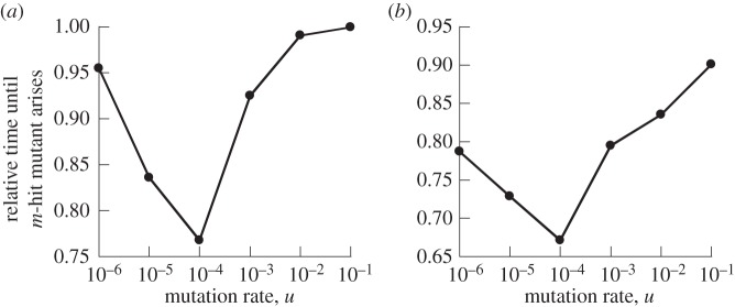
Time to emergence of m-hit mutant in (a) the Moran process and (b) the contact process, assuming that intermediate mutants are advantageous compared with the wild-type, and that the m-hit mutant is even more advantageous. Compared are mass action relative to extreme spatial restriction, where the neighbourhood radius is 1. The time to emergence for radius = 1 was set to unity, and the time observed for mass action was scaled accordingly. This number is plotted against the mutation rate, u. The other parameters were assigned the following values: m = 2, grid size N = 50 × 50, intermediate mutants have 10% fitness advantage. For (b) L/D = 3.

4.1. High mutation rates

Advantageous intermediate mutants are selected for and grow (almost) deterministically rather than drifting. For very high mutation rates, the production of the intermediate mutants by de novo mutations from wild-type also contributes to this growth, and in fact is the dominant force as long as (figure 10a). As explored in the previous sections, mutant growth by production from wild-type is not influenced by the spatial configuration, explaining the small difference between the spatial and mass-action simulations for high mutation rates. For the parameters in figure 9a, we can see that the difference between the mass action and the nearest-neighbour model is small for .

Figure 10.

Time-series simulations showing the evolutionary dynamics for the Moran process, assuming that intermediate mutants are advantageous and the m-hit mutant is even more advantageous. Plots are shown for three mutation rates: (a) 10⁻², (b) 10⁻⁴ and (c) 10⁻⁶. Wild-types are shown in black, intermediate mutants (i.e. one-hit mutants) in blue, and m-hit mutants in green. The simulations were done with m = 2, a 50 × 50 grid, and a 10% fitness advantage of intermediate mutants compared with wild-types. (Online version in colour.)

4.2. Intermediate mutation rates

In this regime, replication rather than de novo production of the intermediate mutants drives growth. The production of m-hit mutants in this regime typically happens by tunnelling (figure 10b). As seen in figure 9, for intermediate mutation rates, systems with spatial structure produce m-hit mutants slower than the mass-action model. The reason for that, interestingly, is the existence of mutant islands. Advantageous intermediate mutants in the spatial systems tend to expand, but they can do so only by growing on the outer rims of the mutant islands (the so-called surface growth; [31]). On the contrary, in the mass-action systems, the mutants experience a bulk growth, leading to a faster (exponential) expansion. The existence of mutant islands served to accelerate the production of m-hit mutants for the neutral and disadvantageous case, because of their protective role. For advantageous intermediate mutants, these islands constrain the growth, slowing down the evolution compared with the mass-action system.

4.3. Low mutation rates

For very low mutation rates, fixation of the intermediate mutant often occurs before the generation of the m-hit mutant (figure 10c). As explored above, this reduces the influence of the neighbourhood radius on the rate of evolution, explaining the reduced difference at low mutation rates. This happens when the characteristic fixation time, uρ^{0 →1}, becomes comparable to the tunnelling rate (which for m = 2 is given by [32] in the case of advantageous mutations). It is easy to show that the effect of sequential fixation becomes dominant if (which for the parameters in figure 9 gives the estimate ).

In the contact process (figure 9b), the same effects take place as described above for the Moran process. The difference is that, in the contact process, there is an additional effect whereby the dynamics in the mass-action model always happens faster than in the spatially restricted systems. As explained before, this happens because of the uniform distribution of individuals across the grid in the mass-action model, which increases the probability of successful reproduction events. Because this effect combines in a positive way with the effects described for the Moran process, the overall effect in the contact process is more significant than in the Moran process. In the contact process, we observe that the evolution happens faster in the mass-action system across all mutation rates, with the effect being the strongest for the intermediate values of u.

5. Discussion

The evolution of complex phenotypes and the crossing of fitness valleys are important evolutionary processes that occur in a variety of populations and organisms [1]. Much of our understanding of the evolutionary dynamics of complex traits has resulted from the analysis of mathematical and population genetic models. Many environments and population interactions are characterized by spatial structure, which is known to influence the outcome of population dynamics in a variety of settings [33]. Here, we extended previous analyses which have studied the role of spatial interactions for the rate at which complex traits evolve [20–22]. A biologically very important message is that the effect of spatial structure on the rate of evolution can crucially depend on assumed population growth laws. This is especially true for neutral and disadvantageous intermediate mutants. For the Moran process, spatial restriction accelerates the evolution of the complex trait. For the contact process, spatial restriction can monotonically accelerate or slow down the rate of evolution, or an intermediate level of spatial restriction can optimize the rate of evolution. Which result is observed depends on parameters, most importantly the rate at which mutations are accumulated. In contrast to neutral and intermediate mutations, spatial restriction always delays the emergence of complex traits if intermediate mutants are advantageous, in both the Moran and the contact process. All these trends are summarized in the schematic in figure 11.

Figure 11.

A schematic summarizing the complex role of space in the generation time of m-hit mutants. The top row represents the Moran process, and the bottom row the contact process. The left column corresponds to neutral/disadvantageous intermediate mutants, and the right column to the advantageous intermediate mutants. In each graph, the horizontal axis represents the degree of mixing, from the nearest-neighbour model to the mass-action model. The curves show whether the waiting time increases or decreases (or is non-monotonic) as a function of the neighbourhood size. It also shows the relative size of the effect, when comparing the Moran process with the contact process.

In the following, we discuss how our results can provide insights into specific biological questions.

5.1. Somatic evolution in tissue

The Moran process is thought to be a good model for the accumulation of mutations in healthy tissue cells that can lead to the generation of cancer [12,13,22,34–38]. Uncontrolled cell growth and cancer development typically require the sequential accumulation of several mutations, and intermediate genotypes can suffer a fitness cost. For example, the inactivation of tumour suppressor genes is crucial in the development of many cancers. Two copies of a tumour suppressor gene need to be inactivated in order for the cell to lose the function mediated by the gene. Inactivation of the tumour suppressor gene can occur through the loss of genetic material by various forms of deletions. If only one copy has been lost (e.g. by a loss-of-chromosome event), other genes can also be lost, leading to a fitness disadvantage of the cell compared with the wild-type. When the second copy of the tumour suppressor gene has been deleted, however, the cell experiences a fitness advantage, because it can now break out of homeostatic control. The assumptions of the Moran model correspond well to the evolutionary dynamics that occur in healthy tissue. Healthy tissue is tightly regulated by feedback factors, such that the number and density of cells remains constant over time, with all the available tissue space filled with cells [39]. Most tissue in the human body exhibits strong spatial structure. Interestingly, our theory suggests that this can minimize the time until a certain number of mutations have accumulated in a cell, and this could reduce the time to cancer. At the same time, however, extensive cell migration occurs in many tissues, and migration has been shown to lead to similar properties as mass action [23]. In addition, it has recently been shown that a hierarchical organization of cell lineages can significantly reduce the rate of double-hit mutant generation [40]. Thus, it is possible that while strong spatial structure is necessary for tissue function for other reasons, patterns of cell organization and cell migration have evolved in order to counter the tumour-promoting effect of spatial structure. Our theory adds to the understanding of the relationship between tissue structure/architecture, rates of evolution and the risk of cancer development.

5.2. Sedentary versus planktonic lifestyles of microbes

While the Moran process is good description of highly regulated tissue growth where space is packed with cells, it is probably a less accurate description of many ecological systems, where not all space of a habitat is occupied by organisms. Instead, there is likely to be a certain spatial distribution of individuals, with the occurrence of empty space. This situation probably applies to free living organisms, for example microbial communities. This scenario is more accurately described by the contact process. As mentioned above, the effect of space on the rate of evolution of complex traits in a contact process is different from that in the Moran process. Space can both accelerate or slow down the rate of evolution, or there can be an optimal degree of spatial restriction that maximizes the rate of evolution. How fast microbial populations can adapt by crossing fitness valleys is probably an important force that drives their evolution. An interesting question to consider in the light of our results is the evolution of sedentary versus planktonic life styles in microbes [41]. Sedentary growth is characterized by strong spatial restrictions, whereas planktonic growth is characterized by a strong degree of mixing. According to our analysis, sedentary growth could be favoured if mutation rates are relatively low. This is because, in this case, populations that show distinct spatial structure can adapt faster through accelerated crossing of fitness valleys than populations that mix well. If, however, mutation rates are higher, evolution is faster under mass action than under spatial restrictions. Therefore, for such bacteria, selection could favour a planktonic life style. Our model gives rise to a hypothesis that can be tested by experiment, although factors other than the rate of fitness valley crossing are likely to also influence the evolutionary outcome.

5.3. Implications for biotechnological processes

Our work also has commercial applications in the field of biotechnology. As pointed out by Frean et al. [42], evolution is used in biotechnology in both directed and non-directed experiments in order to achieve particular endpoints, for example the generation of catalytically efficient enzymes. If the evolutionary processes required to achieve the desired endpoint involve the accumulation of more than one mutation, then our analysis provides a framework to determine optimal spatial cell population structures that can be used to yield the desired results fastest.

5.4. Population growth laws and experiments

As discussed above, of particular importance for the effect of space on the rate of evolution are the laws according to which populations grow in spatially restricted settings. It is currently not possible to say whether the Moran and contact processes presented here are sufficiently realistic descriptions of spatial growth in experimental or natural populations. Indeed, different alternatives to the contact process have been studied, which also capture the assumption that populations are not as tightly regulated as in the Moran process. One alternative model is the branching process [43,44]. This process has been extensively explored in evolutionary applications, including mathematical oncology [45,46], and interesting analytical results regarding mutation processes have been obtained [47]. We chose the contact process because it allows for an easy inclusion of different degrees of spatial structure.

In a more general setting, the notion that population growth laws have an important effect on rates of evolution has also been pointed out in different contexts [42,48]. These studies showed that the probability of mutant fixation can be increased by specific spatial structures compared with well-mixed systems. A particular example is the so-called star graph structure, which enhances the fixation probability of advantageous mutants, while it reduces the fixation probability of disadvantageous mutants.

Therefore, to gain insights into the rates of evolution in the specific populations and systems, the population growth laws have to be determined experimentally. In order to do so, new experiments will have to be performed, which involve the tracking of both the number of individuals as well as the spatial patterns that develop over time. Cell cultures or experiments with microorganisms which can be fluorescently labelled [31,49] would be a suitable system to examine this. Indeed, it is likely that spatial population growth is characterized by different laws in different settings, and that the effect on the rate of fitness valley crossing varies across different spatial population growth laws. This can be investigated by further computational models, but the next step is to obtain more experimental information about spatial population growth laws in different organisms and different settings. Our study provides the motivation and the guide for such future experimental work.

References

- 1.Whitlock MC, Phillips PC, Moore FBG, Tonsor SJ. 1995. Multiple fitness peaks and epistasis. Annu. Rev. Ecol. Syst. 26, 601–629. ( 10.1146/annurev.es.26.110195.003125) [DOI] [Google Scholar]
- 2.Weinreich DM, Chao L. 2005. Rapid evolutionary escape by large populations from local fitness peaks is likely in nature. Evolution 59, 1175–1182. [PubMed] [Google Scholar]
- 3.Weissman DB, Desai MM, Fisher DS, Feldman MW. 2009. The rate at which asexual populations cross fitness valleys. Theor. Popul. Biol. 75, 286–300. ( 10.1016/j.tpb.2009.02.006) [DOI] [PMC free article] [PubMed] [Google Scholar]
- 4.Hancock JF. 2003. RAS proteins: different signals from different locations. Nat. Rev. Mol. Cell Biol. 4, 373–385. ( 10.1038/nrm1105) [DOI] [PubMed] [Google Scholar]
- 5.Moolgavkar SH, Luebeck EG. 1992. Multistage carcinogenesis: population-based model for colon cancer. J. Natl Cancer Inst. 84, 610–618. ( 10.1093/jnci/84.8.610) [DOI] [PubMed] [Google Scholar]
- 6.Fernandez CS, et al. 2005. Rapid viral escape at an immunodominant simian-human immunodeficiency virus cytotoxic T-lymphocyte epitope exacts a dramatic fitness cost. J. Virol. 79, 5721–5731. ( 10.1128/JVI.79.9.5721-5731.2005) [DOI] [PMC free article] [PubMed] [Google Scholar]
- 7.Bowen DG, Walker CM. 2005. Mutational escape from CD8+ T cell immunity HCV evolution, from chimpanzees to man. J. Exp. Med. 201, 1709–1714. ( 10.1084/jem.20050808) [DOI] [PMC free article] [PubMed] [Google Scholar]
- 8.Crawford H, et al. 2009. Evolution of HLA-B* 5703 HIV-1 escape mutations in HLA-B* 5703-positive individuals and their transmission recipients. J. Exp. Med. 206, 909–921. [DOI] [PMC free article] [PubMed] [Google Scholar]
- 9.Sutherland IW. 2001. The biofilm matrix—an immobilized but dynamic microbial environment. Trends Microbiol. 9, 222–227. ( 10.1016/S0966-842X(01)02012-1) [DOI] [PubMed] [Google Scholar]
- 10.de Vries A, Flores ER, Miranda B, Hsieh HM, van Oostrom CTM, Sage J, Jacks T. 2002. Targeted point mutations of p53 lead to dominant-negative inhibition of wild-type p53 function. Proc. Natl Acad. Sci. USA 99, 2948–2953. ( 10.1073/pnas.052713099) [DOI] [PMC free article] [PubMed] [Google Scholar]
- 11.Weissman DB, Feldman MW, Fisher DS. 2010. The rate of fitness-valley crossing in sexual populations. Genetics 186, 1389–1410. ( 10.1534/genetics.110.123240) [DOI] [PMC free article] [PubMed] [Google Scholar]
- 12.Komarova NL, Sengupta A, Nowak MA. 2003. Mutation–selection networks of cancer initiation: tumor suppressor genes and chromosomal instability. J. Theor. Biol. 223, 433–450. ( 10.1016/S0022-5193(03)00120-6) [DOI] [PubMed] [Google Scholar]
- 13.Iwasa Y, Michor F, Nowak MA. 2004. Stochastic tunnels in evolutionary dynamics. Genetics 166, 1571–1579. ( 10.1534/genetics.166.3.1571) [DOI] [PMC free article] [PubMed] [Google Scholar]
- 14.Kimura M. 1985. The role of compensatory neutral mutations in molecular evolution. J. Genet. 64, 7–19. ( 10.1007/BF02923549) [DOI] [Google Scholar]
- 15.Barton N, Rouhani S. 1987. The frequency of shifts between alternative equilibria. J. Theor. Biol. 125, 397–418. ( 10.1016/S0022-5193(87)80210-2) [DOI] [PubMed] [Google Scholar]
- 16.Carter AJR, Wagner GP. 2002. Evolution of functionally conserved enhancers can be accelerated in large populations: a population–genetic model. Proc. R. Soc. Lond. B 269, 953–960. ( 10.1098/rspb.2002.1968) [DOI] [PMC free article] [PubMed] [Google Scholar]
- 17.Iwasa Y, Michor F, Nowak MA. 2004. Evolutionary dynamics of invasion and escape. J. Theor. Biol. 226, 205–214. ( 10.1016/j.jtbi.2003.08.014) [DOI] [PubMed] [Google Scholar]
- 18.Durrett R, Schmidt D. 2008. Waiting for two mutations: with applications to regulatory sequence evolution and the limits of Darwinian evolution. Genetics 180, 1501–1509. ( 10.1534/genetics.107.082610) [DOI] [PMC free article] [PubMed] [Google Scholar]
- 19.Gokhale C, Iwasa Y, Nowak MA, Traulsen A. 2009. The pace of evolution across fitness valleys. J. Theor. Biol. 259, 613–620. ( 10.1016/j.jtbi.2009.04.011) [DOI] [PMC free article] [PubMed] [Google Scholar]
- 20.Durrett R, Foo J, Leder K. In preparation. Spatial Moran models. II. Tumor growth and progression.
- 21.Durrett R, Moseley S. In press. Spatial Moran models. I. Stochastic tunneling in the neutral case. Ann. Appl. Probab. [DOI] [PMC free article] [PubMed]
- 22.Komarova NL. 2006. Spatial stochastic models for cancer initiation and progression. Bull. Math. Biol. 68, 1573–1599. ( 10.1007/s11538-005-9046-8) [DOI] [PubMed] [Google Scholar]
- 23.Thalhauser CJ, Lowengrub JS, Stupack D, Komarova NL. 2010. Selection in spatial stochastic models of cancer: migration as a key modulator of fitness. Biol. Direct. 5, 21 ( 10.1186/1745-6150-5-21) [DOI] [PMC free article] [PubMed] [Google Scholar]
- 24.Bramson M, Durrett R, Swindle G. 1989. Statistical mechanics of crabgrass. Ann. Probab. 17, 444–481. ( 10.1214/aop/1176991410) [DOI] [Google Scholar]
- 25.Nowak MA. 2006. Evolutionary dynamics: exploring the equations of life. Cambridge, MA: Harvard University Press. [Google Scholar]
- 26.Antal T, Scheuring I. 2006. Fixation of strategies for an evolutionary game in finite populations. Bull. Math. Biol. 68, 1923–1944. ( 10.1007/s11538-006-9061-4) [DOI] [PubMed] [Google Scholar]
- 27.Wu B, Gokhale CS, Wang L, Traulsen A. 2012. How small are small mutation rates? J. Math. Biol. 64, 803–827. ( 10.1007/s00285-011-0430-8) [DOI] [PubMed] [Google Scholar]
- 28.Liggett TM. 1999. Stochastic interacting systems: contact, voter and exclusion processes. A Series in Comprehensive Studies in Mathematics, vol. 324 Berlin, Germany: Springer. [Google Scholar]
- 29.Boots M, Sasaki A. 2002. Parasite-driven extinction in spatially explicit host–parasite systems. Am. Nat. 159, 706–713. ( 10.1086/339996) [DOI] [PubMed] [Google Scholar]
- 30.Tomé T, de Carvalho KC. 2007. Stable oscillations of a predator–prey probabilistic cellular automaton: a mean-field approach. J. Phys. A Math. Theor. 40, 12901 ( 10.1088/1751-8113/40/43/005) [DOI] [Google Scholar]
- 31.Wodarz D, Hofacre A, Lau JW, Sun Z, Fan H, Komarova NL. 2012. Complex spatial dynamics of oncolytic viruses in vitro: mathematical and experimental approaches. PLoS Comput. Biol. 8, e1002547 ( 10.1371/journal.pcbi.1002547) [DOI] [PMC free article] [PubMed] [Google Scholar]
- 32.Wodarz D, Komarova NL. 2005. Computational biology of cancer: lecture notes and mathematical modeling. Singapore: World Scientific Publishing Company. [Google Scholar]
- 33.Crawley MJ. 1992. Population dynamics of natural enemies and their prey. In Natural enemies: the population biology of predators, parasites and diseases (ed. Crawley MJ.), pp. 40–89. Oxford, UK: Blackwell Scientific Publications; ( 10.1002/9781444314076.Ch3) [DOI] [Google Scholar]
- 34.Nowak MA, Komarova NL, Sengupta A, Jallepalli PV, Shih IM, Vogelstein Bl. 2002. The role of chromosomal instability in tumor initiation. Proc. Natl Acad. Sci. USA 99, 16 226–16 231. ( 10.1073/pnas.202617399) [DOI] [PMC free article] [PubMed] [Google Scholar]
- 35.Novozhilov AS, Karev GP, Koonin EV. 2006. Biological applications of the theory of birth-and-death processes. Brief Bioinform. 7, 70–85. ( 10.1093/bib/bbk006) [DOI] [PubMed] [Google Scholar]
- 36.Traulsen A, Pacheco JM, Dingli D. 2007. On the origin of multiple mutant clones in paroxysmal nocturnal hemoglobinuria. Stem Cells 25, 3081–3084. ( 10.1634/stemcells.2007-0427) [DOI] [PubMed] [Google Scholar]
- 37.Komarova NL. 2007. Stochastic modeling of loss and gain-of-function mutations in cancer. Math. Models Methods Appl. Sci. 17, 1647–1673. ( 10.1142/S021820250700242X) [DOI] [Google Scholar]
- 38.Dingli D, Pacheco JM, Traulsen A. 2008. Multiple mutant clones in blood rarely coexist. Phys. Rev. E 77, 021915 ( 10.1103/PhysRevE.77.021915) [DOI] [PubMed] [Google Scholar]
- 39.Lander AD, Gokoffski KK, Wan FY, Nie Q, Calof AL. 2009. Cell lineages and the logic of proliferative control. PLoS Biol. 7, e1000015 ( 10.1371/journal.pbio.1000015) [DOI] [PMC free article] [PubMed] [Google Scholar]
- 40.Shahriyari L, Komarova NL. 2014. Symmetric vs asymmetric stem cell divisions: an adaptation against cancer? PLoS ONE 8, e76195 ( 10.1371/journal.pone.0076195) [DOI] [PMC free article] [PubMed] [Google Scholar]
- 41.Jefferson KK. 2004. What drives bacteria to produce a biofilm? FEMS Microbiol. Lett. 236, 163–173. ( 10.1016/j.femsle.2004.06.005) [DOI] [PubMed] [Google Scholar]
- 42.Frean M, Rainey PB, Traulsen A. 2013. The effect of population structure on the rate of evolution. Proc. R. Soc. B 280, 20130211 ( 10.1098/rspb.2013.0211) [DOI] [PMC free article] [PubMed] [Google Scholar]
- 43.Kimmel M, Axelrod DE. 2002. Branching processes in biology. Interdisciplinary Applied Mathematics, vol. 19 Berlin, Germany: Springer. [Google Scholar]
- 44.Haccou P, Jagers P, Vatutin VA. 2005. Branching processes: variation, growth, and extinction of populations. Cambridge, UK: Cambridge University Press. [Google Scholar]
- 45.Goldie JH, Coldman AJ. 2009. Drug resistance in cancer: mechanisms and models. Cambridge, UK: Cambridge University Press. [Google Scholar]
- 46.Bozic I, et al. 2010. Accumulation of driver and passenger mutations during tumor progression. Proc. Natl Acad. Sci. USA 107, 18 545–18 550. ( 10.1073/pnas.1010978107) [DOI] [PMC free article] [PubMed] [Google Scholar]
- 47.Antal T, Krapivsky P. 2011. Exact solution of a two-type branching process: models of tumor progression. J. Stat. Mech. 2011, P08018 ( 10.1088/1742-5468/2011/08/P08018) [DOI] [Google Scholar]
- 48.Lieberman E, Hauert C, Nowak MA. 2005. Evolutionary dynamics on graphs. Nature 433, 312–316. ( 10.1038/nature03204) [DOI] [PubMed] [Google Scholar]
- 49.Hofacre A, Wodarz D, Komarova NL, Fan H. 2012. Early infection and spread of a conditionally replicating adenovirus under conditions of plaque formation. Virology 423, 89–96. ( 10.1016/j.virol.2011.11.014) [DOI] [PubMed] [Google Scholar]