

Abstract
The emergence of cooperation in wolf-pack hunting is studied using a simple, homogeneous, particle-based computational model. Wolves and prey are modelled as particles that interact through attractive and repulsive forces. Realistic patterns of wolf aggregation readily emerge in numerical simulations, even though the model includes no explicit wolf–wolf attractive forces, showing that the form of cooperation needed for wolf-pack hunting can take place even among strangers. Simulations are used to obtain the stationary states and equilibria of the wolves and prey system and to characterize their stability. Different geometric configurations for different pack sizes arise. In small packs, the stable configuration is a regular polygon centred on the prey, while in large packs, individual behavioural differentiation occurs and induces the emergence of complex behavioural patterns between privileged positions. Stable configurations of large wolf-packs include travelling and rotating formations, periodic oscillatory behaviours and chaotic group behaviours. These findings suggest a possible mechanism by which larger pack sizes can trigger collective behaviours that lead to the reduction and loss of group hunting effectiveness, thus explaining the observed tendency of hunting success to peak at small pack sizes. They also explain how seemingly complex collective behaviours can emerge from simple rules, among agents that need not have significant cognitive skills or social organization.
Keywords: dynamics of social systems, disruption of collective behaviours, nonlinear dynamics and chaos, phase transition in biological systems
1. Introduction
Why do animals live in groups? A major benefit to many group living species is the emergence of cooperative behaviours which enhance the reproductive survival of individuals living within the group [1]. But, what are the mechanisms by which cooperation, i.e. helping a potential competitor, emerges and stabilizes in collective animal behaviour?
Collective hunting is a common form of animal cooperation [2] which appears with different levels of complexity, ranging from being at the same place at the same time (bats) to cooperation in complementary actions with role differentiation (Carnivora) [3]. The cooperation of multiple hunters presumably sometimes allows them to successfully capture prey that none of them would be able to capture on their own (larger packs have higher success per attempted hunt [4]). This is the benefit of cooperation. On the other hand, those hunting together have to share their spoils [4]; this is the cost of cooperation. Thus, there is a nonlinear relationship between the individual portion of food available after the hunt and the number of individuals participating in the hunt. The trade-offs that are involved here are not the only challenges in explaining hunting cooperation (see, e.g. the effect of scavenging by ravens in [5]). In fact, uncertainty surrounds the advantage of cooperation (i.e. the benefit-to-cost ratio) when hunting in group [4,6]. A recent review in jackals, coyotes, dholes, African wild dogs and wolves suggested that small groups provide the optimal ratio of benefit-to-cost [4].
Wolf-pack hunting is considered an archetype of collective hunting, as is shown by the fact that it is often referenced in discussions of the foraging and capturing strategies of entities ranging from bacteria Myxococcus xanthus [7] to robots [8,9]. In wolves, per capita rate of food intake is maximal for packs of size two (N = 2) [10], but larger groups reduce the loss of food to scavengers [5], and, in African wild dogs, hunting success is maximal for N = 4 [11]. The reason for hunting success to peak at small pack sizes has recently been studied [12]. Two effects have been compared: the effect of individual wolves impeding each other's actions (interference) and the effect of individual wolves that withhold effort during the hunt and simply remain nearby to have access to the kill. The analysis indicated that interference simply did not occur [12], and they concluded therefore that the loss of effective cooperation within hunting groups is due to the presence of wolves that do not participate fully in the hunt.
In this work, we used a simple, homogeneous, particle-based computational model of pack-hunting in wolves to identify a fundamental mechanism by which effective group-cooperation can emerge. Depending on the number of wolves directly involved in the hunt, we show that above a critical number, complex behavioural patterns such as individual role differentiation and a mosaic of collective formations emerge that can lead to a loss of effectiveness of group hunting strategies.
The hunting ethogram of wolf-packs consists of an initial phase where a single prey is isolated from a herd, then a pursuit phase, and finally, a phase where the prey is captured and killed [13]. Here, we consider that wolves have already isolated a prey, so that we assume that there is a group of N wolves pursuing a single prey.
In our model, the interactions between individuals (wolves and prey) are described in terms of attractions and repulsions as follows:
— Wolf–prey interaction. This is an asymmetric interaction: wolves always repulse the prey, and wolves are always attracted by the prey, but, when wolves arrive at a safe distance dc to the prey, they stop approaching the prey, so as not to be harmed by the horns or the legs of the prey. The repulsion that a wolf exerts on the prey is stronger the smaller the distance between them; respectively, the farther the wolf is from the prey, the weaker the attraction of the prey.
— Wolf–wolf interaction. In our model, wolves do not explicitly attract one another at all. In fact, we assume that the unique one-to-one interaction between wolves is of the repulsive kind: when wolves are at a distance da from the prey, wolves move away from each other. This short-range repulsion is due to the need of individual space (see Hediger 1950 in [14]), collision avoidance, to have a better visibility of the prey [3] and, when close to the prey, to leave space to move freely in response to possible attacks from the prey.
The intensity of these interactions depends on the distance between wolf and prey, and, when close to the prey, on the distance between wolves. The critical thresholds of these distances, i.e. dc and da, depend dynamically on the instantaneous circumstances of the hunt and are time-depending variables. For example, when the prey is getting tired, falls down or triggers a counterattack, the safe distance dc(t) varies accordingly (smoothly or abruptly increasing or decreasing). On the other hand, wolves usually start to move away from each other before feeling menaced by defensive reactions of the prey, so that da(t) > dc(t). In nature, wolves do not necessarily have the same behavioural thresholds, so that dc(t) and da(t) may also vary from one wolf to another. However, to our understanding, the character of the variation of da(t) is not clear: a wolf Wi may keep further away from a more athletic wolf Wj to avoid aggression, so that  would be larger than
  ; on the other hand, the wolf Wi may prefer to get close to Wj to feel protected, so that
  would be smaller than
  . The individualized parameter
  can also include the effects of learning and memory of a single wolf Wi along a single hunt, depending on the individual history experienced by the wolf Wi. For example,
  should increase if in the last interval of time (of a given length) the wolf Wi has been kicked by the prey.
In this model, wolves are assumed indistinguishable and interchangeable, and history effects are not taken into account, so no variation of dc and da among wolves is assumed. Thus, a hunt can be seen as dynamic transitions of the wolf-pack between spatial configurations determined by the changing value of dc(t). Our objective in this work is therefore to obtain the stationary states and equilibria of this dynamical system, and to characterize the stable configurations towards which the dynamical system converges when the control parameter dc(t) is kept constant in time.
Recently, we presented a simple particle model which reproduces the typical wolf-pack hunting patterns observed in nature [15]: cursorial pursuit, encircling manoeuvre, relay running and ambushing. Numerical simulations showed that these patterns can be seen as the emerging result of the combination of two simple rules applied to the behaviour of each individual wolf: (i) move towards the prey until a minimum safe distance to the prey dc is reached, and (ii) when at the safe distance dc, move away from the other wolves that are within the safe area [15]. In this previous work, we assumed for simplicity the particular case where both critical distances are equal (da = dc), that is, wolves start to move away from each other only when they are at the safe distance from the prey. Wolf–wolf interaction was then assumed to occur only when two wolves are at the same distance dc from the prey. An important result was that these hunting patterns emerged without adding a hierarchical or other specific social structure to the simulated wolf-packs, and without assuming high cognitive skills for the agents (wolves and prey).
In this paper, we use a continuous formulation of interaction functions (instead of piece-wise linear functions, as it was in our simple previous model), borrowed from the classical self-propelled particle models [16–22], which produce a more realistic behaviour of the agents than in the previous model, with smooth transitions between regions (close/far to the prey). This has allowed us to introduce in the model the ingredient of the critical distance da through a Gaussian function which determines the region where direct wolf–wolf interactions are relevant. We use this more sophisticated but still quite simple model to obtain the spatial configurations that the agents display when a stationary state or an equilibrium are reached for a given size of the pack and a given value of the critical distance dc. We thus perform a classical study of dynamical systems, in which the description of the stable equilibria will provide us with essential information to understand the behaviour of the system when time variation of control parameters and external conditions such as environmental factors (e.g. variations in the ground) or sudden (unpredictable) changes in animal behaviour are taken into account.
The model is kept as simple as possible in order to identify the essential ingredients necessary for producing the observed behavioural patterns. The kinds of inferences that analysis of this model may warrant, for example regarding social structure or cognitive ability, can be clarified by considering hypotheses concerning another kind of feature such as mass. If we were to observe role differentiation emerging in models in which all the wolves have the same mass, then we would be justified in suggesting that role differentiation does not necessarily rely on mass differences. Of course, this argument is valid even though real wolves obviously do vary in mass. The same analysis applies for hierarchical structures and cognitives abilities: if the behavioural patterns emerge without assuming them, then we can say that the patterns do not necessarily rely on them, and we can do so without denying that real wolves have significant cognitive abilities or that real wolf-packs are hierarchically structured.
2. Results
The use of the formulation of continuous interaction functions has allowed us to show analytically that wolves remain confined to a bounded neighbourhood of the prey even if the wolf–wolf interaction is only of the repulsive kind. The first result is thus that the common attraction from the prey is sufficient to induce wolf-pack aggregation around the prey, so that collective motion and cooperation can emerge.
Once we know that wolves aggregate, we want to know under which conditions cooperation emerges and can be sustained. More specifically, assuming that spatial configurations exhibiting more regularity are more conducive to the production of a successful hunt, we want to know how hunting success depends on the number of wolves, i.e. on the pack size. To do that, we have systematically characterized the stable behavioural patterns towards which the system converges for different pack sizes (2 ≤ N ≤ 15, see [23,24]) and critical safe distances dc (figure 1).
Figure 1.

Snapshots of the stable configuration and its orbits for (N, dc) = (5, 1), (7, 1) and (11, 1.2), and dc–N stability diagram of the stable stationary regular polygon (SRP), which is unstable for N > N* = 5 and  (grey region). Black circles denote the bifurcation value
  for each wolf-pack size N; white circles correspond to the snapshots. See figure 2 and movies in the electronic supplementary material. (Online version in colour.)
The second result is that there exists a critical pack size N* (=5) under which the stable configuration of the wolf-pack is a stationary regular polygon (SRP) centred on the prey, where all wolves are at the same distance from the prey (one-orbit phase). For pack sizes above N* there exists a critical value of the safe distance  below which the SRP becomes unstable. When
  , the wolves are distributed in two or more orbits centred on the prey but at different distances from the prey (multiple orbits phase). This phase transition takes place through a supercritical pitchfork bifurcation which gives rise to complex collective behavioural patterns where individual role differentiation emerges. Spatial configurations exhibit privileged or distinguished positions which could be interpreted as apparent leadership (wolves in the inner orbit, closer to the prey) or wolves withholding effort (wolves holding back in outer orbits). Complex patterns include travelling and rotating formations and periodic oscillatory states, where indicators of chaos have been found in our numerical simulations (small differences between two configurations give rise to unpredictable large differences after a short interval of time).
Among the implications of our results is the fact that wolves could in theory hunt cooperatively together even if all members of the hunt were strangers to one another. In addition, in groups larger than N*, a possible consequence of the high complexity of behavioural patterns is that the hunt may be permanently disrupted. It is reasonable to assume that hunting success is more likely to occur when wolves tend to adopt a regular spatial configuration surrounding the prey than when complex and (apparently) chaotic behavioural patterns take place. Our results may thus explain the observed reduction of hunting success in larger packs. Consequently, packing is only likely to be a selective advantage if the pack is small (a family). Furthermore, the emergence of individual role differentiation in our model shows that social structures reported from hunting scenes might be mere artefact of spatial dynamics.
Our results could be relevant for a wide range of disciplines, from ecology to animal behaviour (for the implications for cognition and social structures [3]), swarm robotics (troop and cooperative formations of homogeneous agents with decentralized decisions and minor communication) and statistical physics (stability and morphology of organization of asymmetric self-propelled particle systems [21]).
3. Methods: the model
We use a simple, homogeneous, particle-based computational model where wolves and prey are modelled as particles that interact through smooth attractive and repulsive forces [14–22,25–27].
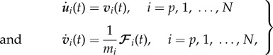
The model equations consist of the Newton's second law for the motion of each individual [14]
| 3.1 |
Here mi is the mass of the ith individual and the vectors  are, respectively, the velocity and the resultant force acting on the ith individual. The index p refers to the prey P. The position of the prey and the N wolves
  is denoted by ui(t) = (xi(t), yi(t)), i = p, 1, … , N. The evolution of the wolves and prey system is thus described by a dynamical system of 2(N + 1) ordinary differential equations
 |
3.2 |
where  includes the individual interactions and the friction with the ground [26]. Note that no alignment forces are assumed and, as we are interested in the stable equilibria towards which the system converges, no noise terms are added [16–18,21,26,27]. Variations of the model that incorporate noise and perturbations, in order to more accurately reflect natural conditions, produce qualitatively the same results but with residual fluctuations around the solution of the zero-noise unperturbed model. See the electronic supplementary material. Wolves and prey in the model have an inner force produced by the metabolism which allows them to move for an unbounded time [27].
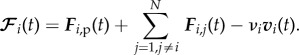
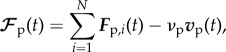
A wolf Wi is subjected to the long-range attractive and short-range repulsive force Fi,p(t) exerted by the prey, the repulsion Fi,j(t) from the other N − 1 wolves and the friction with the ground (e.g. snow) νivi
 |
3.3 |
The interaction functions are defined as smooth functions for positive (non-zero) values of ui
| 3.4 |
| 3.5 |
where g(u) = ga(u) − gr(u), with ga(u) = −u/||u||2 and 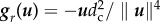 . These interaction functions are a novelty with respect to the piece-wise linear formulation used in [15].
We define also the instantaneous distance Ri(t) from wolf Wi to the prey, Ri(t) = ||ui(t) − up(t)||, and we introduce a Gaussian function ϕij which depends on the relative position of two wolves Wi and Wj with respect to the prey
| 3.6 |
Here dc and da denote the critical safe distance and individual distance described in the Introduction. As mentioned, we assume the general case where dc < da. The Gaussian function ϕij determines the region (of width  ) where wolf–wolf interaction is significant: ϕij(t) is maximal when both wolves Wi and Wj are at a distance da from the prey, and falls rapidly to zero as soon as one of the wolves separates from a distance da to the prey. This is a significant change with respect to the previous model in [15], where da = dc and the width of this region was considered zero. The parameter cw can be made individual-dependent, so that
  would vary from one wolf to another according to the width of the zone of influence we want to assign to wolf Wi. This would be a simple way of introducing an order relation within pack members (i.e. a social structure such as a family or a hierarchy) into the model.
The prey is subjected to the repulsive forces Fp,i(t) exerted by N wolves and the friction with the ground
 |
3.7 |
where Fp,i is colinear to Fi,p but has different intensity:
| 3.8 |
The coefficients  ,
,  and
and  are positive constants describing the relative intensity of the forces, e.g. that the attraction exerted by the prey is stronger than the repulsion that wolves exert on the prey. Although these coefficients should vary in time, we consider that this variation can be neglected with respect to the changes produced by the time variation of dc. Finally, mass and friction m and ν are considered identical for all wolves, and larger for prey than for wolves (mp > mi, νp > νi). Note that these are relative values; agents with a smaller mass can change speed more easily (high acceleration), while agents with a larger friction can change direction more easily (high manoeuvrability).
The values of the parameters are shown in table 1. We have used normalized units to have parameter variations of order one and dc ≈ 1.
Table 1.
Variables and typical values of the parameters.
| mp | mass of the prey (350–400 Kg) | 1 |
| mi | mass of wolf Wi (35–40 Kg) | 0.1 |
| νp | prey friction coefficient | 2 |
| νi | wolf friction coefficient | 1 |

|
coefficient of force that the prey exerts on a wolf | 2 |
 |
coefficient of interaction force between wolves | 0.5 |

|
coefficient of force that a wolf exerts on the prey | 0.2 |
| dc | wolves safe distance not to be harmed by the prey | 1 |
| da | distance to the prey at which wolves repulse each other | 1.5 |
| cw | width coefficient of Gaussian function ϕi,j ( ) ) |
0.5 |
 |
maximum modulus of prey's velocity | 0.1 |
| Ri | radius of the orbit of wolf Wi | approx. 1–2 |
| Rc | radius of the SRP (stationary regular polygon) | approx. 1–2 |
| N | wolf-pack size (number of wolves) | 2–20 |
The interaction function g(u) introduced in the model (instead of the piece-wise formulation used in [15]) is a particular case of the attraction/repulsion function introduced by Shi & Xie [16], which in turn belongs to a class of interaction functions in swarm aggregation described by Gazi & Passino [17,18] in models with no friction where a very small individual mass moving in a medium of high viscosity (e.g. bacteria) is assumed (m ≈ 0). Under some conditions, such an interaction function can exhibit the basic features of stability and cohesion of the swarm [18]. Liu et al. [19] also presented an interaction function which precludes agents from colliding with one another: the repulsion grows to infinite as the distance between agents goes to zero. The interaction function of Shi & Xie [16] provides a more realistic behaviour at long distances: the intensity of the interaction between agents goes to zero as the distance between them grows to infinite. Here, we use g(u) and the inertial system (3.2) instead of the reduced system proposed in [18]. A similar combination has been used recently [20] in an inspiring numerical study of collective behaviour of prey in the presence of predators in the case of single predator–single prey, single predator–multiple prey and multiple predator–multiple prey, surprisingly omitting the multiple predators–single prey case studied here.
3.1. Wolf-pack cohesion
When interactions are symmetric, it is often possible to show that the swarm has a stationary centre around which individuals aggregate [16–19]. However, this is not the case in our wolves–prey system, which is not symmetric. Moreover, during a hunt, wolves do not tend to attract other wolves but rather, when there is an interaction, the tendency is towards repulsion. We thus consider that wolf–wolf interactions are only of the repulsive kind. In spite of that, our results show that wolves swarm into a wolf-pack formation because of their common interest in approaching the prey [4].
Definition 3.1. —
A wolf Wi is said to be a free agent [17] if Wi is far enough from P so that the repulsion from other wolves is negligible with respect to the attraction from the prey: Ri ≥ δ, for an arbitrarily large positive constant
.
Proposition 3.2. —
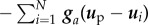
If Wi is a free agent, then the Newton's second law for Wi can be written as follows:
3.9 Proof. When δ → + ∞, on the one hand,
3.10 so
, and thus g(ui − up) ≈ ga(ui − up), and on the other hand,
3.11 so
, j ≠ i.
Definition 3.3. —
Let
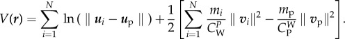
in
and
the potential functional (which is not a Lyapunov function) defined as
3.12
Lemma 3.4. —
If mi/mp < νi/νp < 1, then
3.13 implies
3.14
Condition (3.13) can be viewed as a refinement of  . Reasonably, the larger the number of wolves, the smaller can be their velocity to satisfy (3.13), i.e. wolves in larger packs do not need to run at such high speeds. Prey would not run faster when escaping from N + 1 wolves than when escaping from N wolves. Condition (3.13) is less restrictive for wolves' velocity than imposing that the sum of the velocities of the wolves is greater than the prey's velocity because
  and mi/mp < 1.
Theorem 3.5. —
If Wi is a free agent and the velocity of the prey is bounded from above (i.e.
), then, for typical masses and friction coefficients, V(r) is bounded from below and
along free agents trajectories.
Proof. —
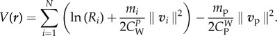
The potential function V(r) can be written as
3.15
Typical values of mass and friction coefficients for wolves and prey (e.g. moose, elk—Alces alces) are such that mi/mp < νi/νp (see parameter values in table 1), so, by lemma 3.4, both conditions (3.13) and (3.14) hold. Then, the expression between brackets in (3.15) is positive and, for free agents, we have V(r) ≥ N ln(δ), so that, for free agents, the potential function V(r) is bounded from below.
On the other hand, the time-derivative of V(r) along the trajectories of free agents is given by
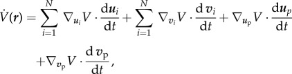 |
where 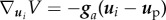 ,
, 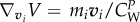 ,
, 
 and
and  . Then
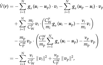 |
which, as (3.14) holds, is negative.
Theorem 3.5 shows that the function V(r) is strictly decreasing and bounded from below, so it converges to a minimum that is reached when all the wolves are at a distance δ from the prey, meaning that free agents move towards the ball of radius δ centred in P.
Thus, wolf-pack aggregation takes place during hunting and is not necessarily owing to the attraction between wolves; pack-hunting can be a contingency where wolves hunt in a particular location simply because food is there (like M. xanthus [7]).
3.2. Stability of wolf-pack configurations
Once we know that wolves aggregate around the prey, we want to know which kind of spatial configuration they exhibit when a stable equilibrium is reached. Results of stability have already been reported for symmetric interactions [21,22]. When interactions are asymmetric, analytical tools are more difficult to use and we have to rely on numerical simulations.
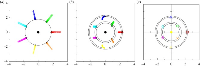
Figure 2 shows the time-evolution of the wolves and prey system for N = 5, 6 and 7 for the initial condition ui(0) = (0.5i − 4, − 0.35), i = 1, … , N in a square domain of dimensionless size 8 (large enough compared with the typical distance dc ≈ 1).
Figure 2.

Convergence of the initial configuration ui = (0.5i − 4, − 0.35), i = 1, …, N, to the stable state. For dc = 1.3 (a–c), the final state is the SRP. For dc = 1 (d–f), the SRP loses its stability for N > 5. (a) N = 5, radius of the SRP: Rc = 1.78. (b) N = 6, Rc = 1.9. (c) N = 7, Rc = 2. (d) N = 5, Rc = 1.41. (e) N = 6, stationary two-orbits configuration with R1,2,3 = 1.29 and R4,5,6 = 1.91. (f) N = 7, stable flocking four-orbits configuration with R1,2 = 1.26, R3,4 = 1.46, R5,6 = 2.18 and R7 = 2.33. Flocking velocity is  and
and  (i.e. ||vi|| = 3.6 × 10⁻²). (Online version in colour.)
Each simulation in figure 2 shows the trajectory followed by each wolf with respect to the prey until an equilibrium between all agents is reached. The spatial configurations displayed by the N wolves and the prey are represented in figures and movies as centred on the prey, so that the prey is located in the origin (0, 0) with zero velocity.
The initial condition is taken such that not all the wolves are aligned with the prey, and such that wolves do not describe a regular polygon centred on the prey. If these conditions are not fulfilled, unrealistic solutions arise: if wolves are initially aligned with the prey, then they never leave this line; and if wolves initially describe a regular polygon around the prey, then they converge to the SRP corresponding to the values of N and dc, even if the SRP is unstable (figure 3).
Figure 3.
Initial configuration with the form of a regular polygon centred on the prey, for N = 7, dc = 1 and initial radius R = 3. (a) The wolf-pack converges to the corresponding SRP, where R = 1.79214179. (b) Unstability of the SRP under a perturbation of order 10−6 in the abscissa of the position of only one wolf: the wolf-pack converges to the stable four-orbits configuration, already shown in figure 2f. (c) Final configuration, with R1,2 = 1.26, R3,4 = 1.46, R5,6 = 2.18 and R7 = 2.33. The configuration is symmetric with respect to the axis of abscissa. (Online version in colour.)
We have used a first-order explicit Euler method with a small time-step Δt = 10−6. The numerical test for equilibrium is
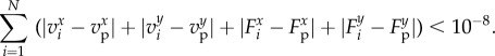 |
We would like to stress that these trajectories should not be interpreted as displaying the successive positions of wolves during real hunts; what these simulations show is the convergent process of the dynamical system towards the stable configuration corresponding to the given value of (N, dc).
We have carried out numerical simulations of the wolves and prey system for a wide range of values of dc for different pack sizes, obtaining for each case the resulting stable configuration adopted by the system. The final configuration does not depend on the initial condition, except rotations (i.e. variations of the angle described by the formation with respect to the horizontal line). We have then characterized the final stable configurations by measuring the radius of the orbit in which each wolf is located. The result is the so-called R–dc stability curve of the SRP for each pack size N = 2 − 20. See figure 3 for pack sizes N = 2, 3, 4, 5, 8 and 11.
We observe that in small packs, the radius Rc of the SRP grows smoothly and almost linearly with dc (see figure 4 for N ≤ N* = 5), while for pack sizes larger than N*, the SRP loses its stability via a supercritical pitchfork bifurcation [28] at  (see figure 4 for N = 8 and N = 11).
Figure 4.
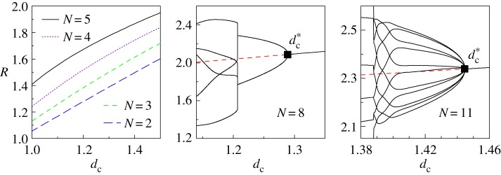
Radii of the stable configurations and the SRP for different pack sizes (R–dc stability curve). For small packs (N ≤ N* = 5), only the SRP is stable. For N > N* = 5, there is a supercritical pitchfork bifurcation at  (black square) and the SRP is unstable (dashed line for N = 8 and N = 11 showing the radius Rc of the SRP). For N = 8, the bifurcation gives rise to two orbits with four wolves per orbit, while for N = 11, it leads to 11 orbits with one wolf per orbit. (Online version in colour.)
Figure 1 shows the value of  for different pack sizes. We have analysed the stable configurations corresponding to
  , obtaining that the wolves are distributed in several orbits centred on the prey and display complex dynamical patterns, including flocking (travelling with constant speed), milling (rotating around a point or a region), periodic oscillations and (possible) chaos (where small differences between configurations give rise to unpredictable large differences [28]).
Figure 5 shows the R–dc curve for N = 6. When  , the SRP is unstable and wolves are distributed around the prey P in multiple orbits of different radii
  , Ri < Ri
+
1, 2 ≤ m ≤ N. Insets show the simplest stable multi-orbital formations, which can be (i) stationary (vi,p = 0), (ii) flocking (with constant speed vi = vp = vf) or (iii) milling (rotating around P). See the electronic supplementary material, movies M1 and M2.
, Ri < Ri
+
1, 2 ≤ m ≤ N. Insets show the simplest stable multi-orbital formations, which can be (i) stationary (vi,p = 0), (ii) flocking (with constant speed vi = vp = vf) or (iii) milling (rotating around P). See the electronic supplementary material, movies M1 and M2.
Figure 5.

R–dc curves for N = 6. Supercritical pitchfork bifurcation (square) at  . Solid lines, stable radii Ri; dashed line: unstable Rc; vertical dot-dashed lines, regions of qualitatively different patterns shown in the insets (diamonds): (a) SRP at (dc, Rc) = (1.3, 1.9). (b) Stationary multi-orbital configuration for dc = 1, R1 = 1.29, R2 = 1.91 (m = 2, three wolves per orbit). (c) Stable counterclockwise vortex for dc = 0.821, rotating along six orbits (R1 ≈ R2 ≈ R3 < Rc < R4 < R5 < R6). In insets, the central star denotes prey location. (Online version in colour.)
We would like to stress that although they are not stationary, the flocking, milling and (apparently) chaotic configurations are stable configurations, in the sense that for a given value of (N, dc), the wolves and prey system converges to the corresponding configuration until this dynamical equilibrium is reached. See the analysis of the influence of adding noise to the equations of prey and wolves and perturbations to the behaviour of the prey (sudden jumps) in the electronic supplementary material.
Pattern diversity and complexity increase in larger packs. Figure 6a shows a stable periodic oscillatory state for N = 7 where four wolves shuttle between the inner and outer orbits, while two wolves stand still in the inner orbit and the last one moves quickly along a short arc of the outer orbit. Figure 6b shows a time parametric representation of radii (stroboscopic map) illustrating periodicity, and figure 6c shows the oscillations' frequencies. The dynamics of this solution is shown in the electronic supplementary material, movie M3.
Figure 6.

Stable periodic oscillations for N = 7 and dc = 0.78. (a) Wolves trajectories: small numbers denote number of wolves per trajectory. (b) Stroboscopic map R1(t) versus R2(t) (dashed line) and R1(t) versus R3(t) (solid line). (c) Oscillations of Ri(t) m = 3 showing 4, 7 and 14 periods. (Online version in colour.)
Figure 7 corresponds to a large pack (N = 12) for which a possible route to chaos has been found. Figure 7a–c shows the trace of wolves' trajectories at different instants of time for dc = 1.3. See the dynamics in the electronic supplementary material, movie M4. The stroboscopic maps shown in figure 8 illustrate the high sensitivity of the system under small variations of dc and reveal a possible route to chaos close to dc = 1.3. We would like to stress again that this solution is stable, meaning that for this value of (N, dc) = (12, 1.3) and whatever initial condition (except wolves aligned with the prey or displaying a regular polygon centred on the prey), the system will exhibit a qualitatively identical (apparently chaotic) behaviour.
Figure 7.
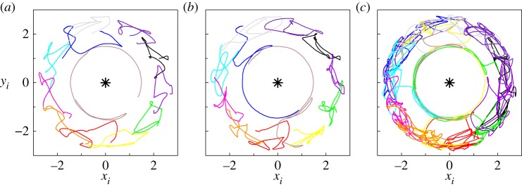
(a–c) Highly complex behavioural patterns for dc = 1.3, exhibiting apparent relays and leading role in a pack of 12 wolves behaving (possibly) chaotically. (Online version in colour.)
Figure 8.
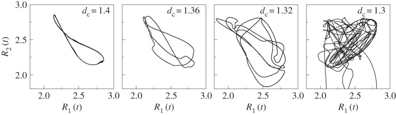
Stroboscopic maps for N = 12 revealing a possible route to chaos as dc decreases from 1.4 to 1.36, 1.32 and 1.3.
4. Discussion
We have shown that provided the (analytically derived) condition (3.13) for the relative velocities of the agents is satisfied, wolves do not escape to infinity and are confined to a bounded neighbourhood of the prey. Thus, during hunts, wolf-pack cohesion always takes place and is maintained even if the wolf–wolf interactions are only of the repulsive kind. This confinement gives rise to a pléiade of collective behavioural patterns which, under small variations of the parameters of the model, converge towards specific spatial configurations. We have then studied the stability of the stationary states and equilibria of the wolves and prey system, characterizing the spatial configurations towards which the system converges for a given size of the pack and a given critical safe distance dc.
The stability analysis revealed that, for small packs, small variations of the safe distance dc induce small variations of the radii of the orbits Ri, so that the hunt evolves smoothly and straightforwardly. Meanwhile, for large packs, small variations of dc can induce dramatic qualitative and quantitative changes in the spatial configuration of the wolf-pack. Our main results suggest that, observed in nature, these abrupt variations can contribute to disruptions of the hunt, therefore reducing the hunting success. One thus expects hunting groups to be limited to sizes that permit hunts to proceed without disruption.
MacNulty et al. [12] show empirically that the success of wolves hunting elk reaches its maximum value at four to five wolves because for larger group sizes (N > 5) some individuals start to withhold hunting effort. A possible interpretation of our results is that the complex spatial dynamics displayed by the stable configuration in large packs (N > 5) may contribute to the observed tendency of hunting success to peak at small packs by triggering specific spatial patterns which facilitate freeriding: individuals travelling or being located in the outer orbits of large packs (N > 5) may more easily withhold effort than individuals located in the inner orbit because they are further from the prey, whereas individuals in the single orbit of a small pack (N ≤ 5) probably have more incentive to fully contribute to the hunt. Consequently, complex spatial dynamics can facilitate freeriding events in large packs, which in turn induce a decrease in hunting success in large packs.1
On the other hand, behavioural patterns like those simulated in figure 6 look surprisingly like a socially structured group. A possible scenario for figure 6a could be as follows: a breeding pair stands (almost) still in the inner orbit, leading or conducting the hunt, while four inexperienced offspring move back and forth from the inner orbit to the outer and vice versa, and a single excited juvenile (see the frequency of its oscillations and the distance it travels in figure 6b,c) remains protected behind its progenitors. Other patterns like those shown in figure 7 might suggest a series of successive relays in the leading role.
Our results show, however, that such patterns emerge in our numerical simulations from spatial dynamics alone. Such scenarios should be understood as the underlying stable states which, in combination with time variations of the control parameters (mainly dc(t)) and the possible contribution of behavioural phenomena, are the attractors2 of the collective behaviours observed in nature.
The previous model [15] already displayed collective hunting-like behaviours, such as leadership, relay running and ambushing. Our present model expands on this previous work by using more realistic parameters for wolf–wolf and wolf–prey interactions. Specifically, it allows for a smooth transition between areas where the direct wolf–wolf interaction is significantly different (i.e. when Ri is close to da) and for a more realistic behaviour of the prey. Moreover, this work allows for a richer dynamic structure of spatial configurations. It has also revealed a possible mechanism by which role differentiation can arise as an emergent behaviour of collective hunting; this results in our model from the successive bifurcations into multiple branches in the R–dc curve.
The differentiation of privileged orbits could alternatively be interpreted as being the result of the social structure of the hunting pack. Our results illustrate that social structure is not necessary. Nevertheless, it is possible that the mechanisms underpinning our model may interact with the pack social structure in real life situations, in such a way that some individuals end up in privileged locations more frequently than others.
The rich variety of patterns displayed by larger packs demonstrates why wolf-pack hunting is often interpreted in terms of strategies, such as foresight, planning or purposiveness.
Without ruling out the importance of social structures and cognitive abilities, we propose to incorporate a fundamental ingredient to the behavioural interpretations of wolf-pack hunting patterns: the emergent contribution of the combination of simple mechanical rules.
Acknowledgements
We thank Lorna Coppinger and Annick Laruelle. We thank also two of the anonymous referees for insightful comments that improved our paper. Any opinions, findings, and conclusions or recommendations expressed in this publication are those of the authors and do not necessarily reflect the views of the National Science Foundation.
Endnotes
We thank one of the anonymous referees for pointing out this interpretation of our results.
In nonlinear dynamics, an attractor is a set to which all neighbouring trajectories converge [28].
Funding statement
Material based on work supported by National Science Foundation, grant nos. 1017817 and 1129139.
References
- 1.Nowak MA. 2006. Five rules for the evolution of cooperation. Science 314, 1560–1563. ( 10.1126/science.1133755) [DOI] [PMC free article] [PubMed] [Google Scholar]
- 2.Packer C, Ruttan L. 1988. The evolution of cooperative hunting. Am. Nat. 132, 159 ( 10.1086/284844) [DOI] [Google Scholar]
- 3.Bailey I, Myatt JP, Wilson AM. 2013. Group hunting within the Carnivora: physiological, cognitive and environmental influences on strategy and cooperation. Behav. Ecol. Sociobiol. 67, 1–17. ( 10.1007/s00265-012-1423-3) [DOI] [Google Scholar]
- 4.MacDonald DW, Creel S, Mills MGL. 2004. Canid society In The biology of conservation of wild canids (eds MacDonald DW, Sillero-Zubiri C.), pp. 85–106. Oxford, UK: Oxford University. [Google Scholar]
- 5.Vucetich JA, Peterson RO, Waite TA. 2004. Raven scavenging favours group foraging in wolves. Anim. Behav. 67, 1117–1126. ( 10.1016/j.anbehav.2003.06.018) [DOI] [Google Scholar]
- 6.Fryxell JM, Mosser A, Sinclair ARE, Packer C. 2007. Group formation stabilizes predator–prey dynamics. Nature 449, 1041–1043. ( 10.1038/nature06177) [DOI] [PubMed] [Google Scholar]
- 7.Berleman JE, Kirby JR. 2009. Deciphering the hunting strategy of a bacterial wolfpack. FEMS Microbiol. Rev. 33, 942–957. ( 10.1111/j.1574-6976.2009.00185.x) [DOI] [PMC free article] [PubMed] [Google Scholar]
- 8.Madden JD, Arkin RC, MacNulty DR. 2010. Multi-robot system based on model of wolf hunting behavior to emulate wolf and elk interactions. In IEEE Int. Conf. on Robotics and Biomimetics (ROBIO 2010), Tianjin, China, 14–18 December 2010, pp. 1043–1050 ( 10.1109/ROBIO.2010.5723472) [DOI] [Google Scholar]
- 9.Weitzenfeld A, Vallesa A, Flores H. 2006. A biologically-inspired wolf pack multiple robot hunting model. In IEEE 3rd Latin American Robotics Symposium (LARS 2006), Santiago, Chile, 26–27 October 2006, pp. 120–127 ( 10.1109/LARS.2006.334327) [DOI] [Google Scholar]
- 10.Peterson RO, Ciucci P. 2003. The wolf as a carnivore. In Wolves: behavior, ecology and conservation (eds Mech LD, Boitani L.), pp. 104–130. Chicago, IL: University of Chicago Press. [Google Scholar]
- 11.Fanshawe JH, FitzGibbon CD. 1993. Factors influencing the success of an African wild dog pack. Anim. Behav. 45, 479–490. ( 10.1006/anbe.1993.1059) [DOI] [Google Scholar]
- 12.MacNulty DR, Smith DW, Mech LD, Vucetich JA, Packer C. 2012. Nonlinear effects of group size on the success of wolves hunting elk. Behav. Ecol. 23, 75–82. ( 10.1093/beheco/arr159) [DOI] [Google Scholar]
- 13.MacNulty DR, Mech LD, Smith DW. 2007. A proposed ethogram of large-carnivore predatory behavior, exemplified by the wolf. J. Mammal 88, 595–605. ( 10.1644/06-MAMM-A-119R1.1) [DOI] [Google Scholar]
- 14.Gueron S, Levin SA, Rubinstein DI. 1996. The dynamics of herds: from individuals to aggregations. J. Theor. Biol. 182, 85–98. ( 10.1006/jtbi.1996.0144) [DOI] [Google Scholar]
- 15.Muro C, Escobedo R, Spector L, Coppinger RP. 2011. Wolf-pack (Canis lupus) hunting strategies emerge from simple rules in computational simulations. Behav. Proc. 88, 192–197. ( 10.1016/j.beproc.2011.09.006) [DOI] [PubMed] [Google Scholar]
- 16.Shi H, Xie G. 2011. Collective dynamics of swarms with a new attraction/repulsion function. Math. Probl. Eng. 735248, 021110. [Google Scholar]
- 17.Gazi V, Passino KM. 2003. Stability analysis of swarms. IEEE Trans. Automatic Control 48, 692–697. ( 10.1109/TAC.2003.809765) [DOI] [Google Scholar]
- 18.Gazi V, Passino KM. 2004. A class of attractions/repulsion functions for stable swarm aggregations. Int. J. Control 77, 1567–1579. ( 10.1080/00207170412331330021) [DOI] [Google Scholar]
- 19.Liu B, Chu T-G, Wang L, Wang Z-F. 2005. Swarm dynamics of a group of mobile autonomous agents. Chin. Phys. Lett. 22, 254–257. ( 10.1088/0256-307X/22/1/073) [DOI] [Google Scholar]
- 20.Zhdankin V, Sprott JC. 2010. Simple predator–prey swarming model. Phys. Rev. E 85, 056209 ( 10.1103/PhysRevE.82.056209) [DOI] [PubMed] [Google Scholar]
- 21.D'Orsogna MR, Chuang YL, Bertozzi AL, Chayes L. 2006. Self-propelled particles with soft-core interactions: patterns, stability, and collapse. Phys. Rev. Lett. 96, 104302 ( 10.1103/PhysRevLett.96.104302) [DOI] [PubMed] [Google Scholar]
- 22.Chen H-Y, Leung K. 2006. Rotating states of self-propelling particles in two dimensions. Phys. Rev. E 73, 056107 ( 10.1103/PhysRevE.73.056107) [DOI] [PubMed] [Google Scholar]
- 23.Mech LD, Boitani L. 2003. Wolf social ecology. In Wolves: behavior, ecology and conservation (eds Mech LD, Boitani L.), pp. 1–34. Chicago, IL: University of Chicago Press. [Google Scholar]
- 24.Mech LD, Boitani L. (eds) 2003. Wolves: behavior, ecology and conservation. Chicago, IL: University of Chicago Press. [Google Scholar]
- 25.Vicsek T, Zafeiris A. 2012. Collective motion. Phys. Rep. 517, 71–140. ( 10.1016/j.physrep.2012.03.004) [DOI] [Google Scholar]
- 26.Levine H, Rappel W-J, Cohen I. 2001. Self-organization in systems of self-propelled particles. Phys. Rev. E 63, 017101 ( 10.1103/PhysRevE.63.017101) [DOI] [PubMed] [Google Scholar]
- 27.Sprott JC. 2009. Anti-Newtonian dynamics. Am. J. Phys. 77, 783 ( 10.1119/1.3157152) [DOI] [Google Scholar]
- 28.Strogatz SH. 1994. Nonlinear dynamics and chaos. Boulder, CO: Westview Press. [Google Scholar]