Prospective Motion Correction using Inductively-Coupled Wireless RF Coils

Abstract

Purpose

A novel prospective motion correction technique for brain MRI is presented that uses miniature wireless radio-frequency (RF) coils, or “wireless markers”, for position tracking.

Methods

Each marker is free of traditional cable connections to the scanner. Instead, its signal is wirelessly linked to the MR receiver via inductive coupling with the head coil. Real-time tracking of rigid head motion is performed using a pair of glasses integrated with three wireless markers. A tracking pulse-sequence, combined with knowledge of the markers’ unique geometrical arrangement, is used to measure their positions. Tracking data from the glasses is then used to prospectively update the orientation and position of the image-volume so that it follows the motion of the head.

Results

Wireless-marker position measurements were comparable to measurements using traditional wired RF tracking coils, with the standard deviation of the difference < 0.01 mm over the range of positions measured inside the head coil. RF safety was verified with B₁ maps and temperature measurements. Prospective motion correction was demonstrated in a 2D spin-echo scan while the subject performed a series of deliberate head rotations.

Conclusion

Prospective motion correction using wireless markers enables high quality images to be acquired even during bulk motions. Wireless markers are small, avoid RF safety risks from electrical cables, are not hampered by mechanical connections to the scanner, and require minimal setup times. These advantages may help to facilitate adoption in the clinic.

INTRODUCTION

Head motion is a fundamental problem for all in vivo brain MRI applications that, if left unaccounted for, can result in high clinical and public health costs. Even a few millimeters of movement can produce severe motion artifacts that can mask subtle lesions, obscure pathologies, or simply lower diagnostic confidence. A motion correction solution has yet to be demonstrated that is comprehensive, simple to deploy, and widely accepted in the clinic.

The use of miniature radio-frequency (RF) coils as position-tracking probes (1,2) has been the foundation of several recent advances in prospective real-time motion correction (3–14). We refer to these previously developed RF coils (1–14) as “wired markers”, since each RF coil was connected to the scanner via a traditional coaxial cable. In our previous works (5–9,14), subjects wore a headband containing three wired markers, which served as the fiducial for head motion tracking. Prospective correction for rigid head motions, using the real-time tracking data from the wired markers, was successfully implemented in a variety of imaging sequences. The technique improved the image quality of 2D/3D structural MRI (5), as well as increased the statistical significance of functional MRI (6,7,14). While wired markers have been effective in a research setting, their widespread adoption may be hampered by the cables connecting the headband to the scanner, which would interfere with the regular clinical workflow.

We therefore introduce a novel RF coil-based “wireless marker” approach for prospective motion correction of brain MRI, which aims to streamline the overall setup procedure. All cable connections to the scanner are eliminated by inductively coupling the wireless markers to the imaging head-coil. Real-time tracking of rigid head motion is performed using a pair of glasses, with three wireless markers integrated into its frame in a predefined geometrical arrangement. A tracking pulse-sequence, combined with knowledge of the markers’ geometrical arrangement, is used to measure their positions. The wireless tracking data from the glasses is then used to prospectively update the image-volume’s orientation and position so that it follows the motion of the head. Inductively-coupled RF-coils (15–18) have been previously used to improve local image SNR (15), visualize stents (17), and catheters (18). We present here the first work to use inductively-coupled RF-coils for prospective real-time tracking and correction of rigid head motion, which expands on our preliminary results (19).

The removal of all cables makes wireless markers substantially easier to use and less cumbersome than wired markers, thereby improving patient comfort, technologist setup times, and tracking fidelity. Patient safety is improved by eliminating the long, electrically conducting cables that are a potential source of RF heating and local SAR increase. Also, by inductively coupling the wireless markers to the imaging head-coil, the load on the scanner is reduced since no additional RF receiver channels or scanner interface circuitry is required. These practical advantages allow the technique to be more easily deployed in a high throughput clinical setting.

METHODS

Experiments were performed on a 3T GE-MR750 scanner (GE Healthcare, WI, USA). A standard 8-channel head-coil was used for imaging and inductive coupling to the wireless markers. All experiments with human subjects were in accordance with local institutional review board (IRB) regulations and informed consent was obtained before each exam.

Wireless Marker Device

Prospective correction is performed using three wireless markers in order to uniquely define any six degrees-of-freedom (6-DOF) rigid-body motion. Each wireless marker (Fig. 1a, bottom) is a miniature RF coil that is free of any mechanical connections to the scanner. It is a three-turn (Ø ~ 4 mm) solenoid inductor, and capacitor, tuned to 128 MHz. Inside the solenoid cavity is a small glass sphere (Ø ~ 3 mm) filled with Gd-doped water solution (10 mM). The spherical sample is the point source that is tracked. A fast-switching crossed diode (UMX9989AP, Microsemi, MA, USA) passively detunes the resonant circuit during RF transmit.

Fig. 1.

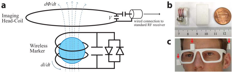
a) Circuit schematic of a single wireless marker (bottom), and illustration of wireless-marker signal transmission by inductively coupling the wireless marker to the imaging head-coil (top). The underlying principle used for wireless-marker tracking is Faraday’s law of mutual induction. During RF receive, each wireless marker picks up the MR signal in its immediate vicinity (dominated by the spherical sample). The signal generates a current di/dt in the wireless marker, and an associated magnetic field (dashed lines) and flux dΦ/dt as it passes through the imaging head-coil. The flux induces a voltage V in the imaging head-coil according to Faraday’s law: di/dt ∝ dΦ/dt ∝ V, which is then routed to the standard RF receiver. The key concept here is that even though these two RF coils are not physically connected, the signal from the wireless marker is transmitted to the imaging head-coil via the magnetic flux dΦ/dt that links the two coils. b) wireless marker (left), enclosing capsule (middle), and U.S. penny (right), relative to ruler markings in mm. c) polycarbonate glasses containing three wireless markers (red arrows) for brain MRI.

In the absence of any cable connections, wireless-marker signal transmission is achieved by inductively coupling the wireless markers to the nearby imaging head-coil. This is illustrated in Fig. 1a. During RF receive, each wireless marker acts as a local signal amplifier that picks up the MR signal in its immediate vicinity, which is dominated by the spherical sample. The signal is then wirelessly transmitted to the imaging head-coil via the magnetic flux dΦ/dt that links the two coils, and thereby routed to the standard RF receiver.

Each wireless marker is encased in a self-contained polycarbonate capsule (Fig. 1b). For phantom experiments, three capsules were rigidly attached to the phantom in a predefined geometrical arrangement. For in vivo experiments, the subject wore a pair of polycarbonate glasses (Fig. 1c) that was custom designed (SolidWorks, MA, USA) and 3D-printed (Stratasys Fortus 360mc, MN, USA) with three capsules integrated into its frame.

Wireless Tracking Signal

Wireless marker positions were measured using the tracking pulse-sequence (5) in Fig. 2a, which produces three 1D projections along the physical x, y, and z gradient axes. We refer to the signal from these 1D projections as the wireless tracking signal S_1–8, since the signal from all three markers is wirelessly received by the 8-channel head coil (receiver channels 1–8) via the inductive coupling mechanism. S_1–8 is calculated from the sum-of-squares (SOS) signal over all 8 channels. S_1–8 from a single x-projection of three markers (Fig. 2b) clearly shows three peaks, which correspond to the marker locations along the physical x-axis. A similar set of peaks in the y- and z-projections provides information on the marker positions in 3D.

Fig. 2.

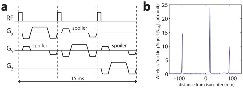
a) The tracking pulse-sequence (5) used to measure wireless marker positions. A non-selective RF-pulse (α = 1°) is followed by gradient-echo readouts along the physical x, y, and z gradient axes (FOV = 300 mm, N = 256), resulting in three 1D projections along orthogonal axes. Spoiler gradients dephase the magnetization in large volumes (from the subject) while preserving signal from the smaller spherical samples inside each marker. b) Wireless tracking signal S_1–8 from three wireless markers after the x-projection of the tracking pulse-sequence. This is the SOS signal received by the 8-ch head coil as it inductively couples with the markers. Three peaks are clearly visible, which correspond to the marker locations along the x-axis. Background signal from the phantom is well suppressed by the spoilers.

However, from S_1–8 alone it is not immediately obvious which peak corresponds to which marker, since the signals from all three markers are simultaneously coupled to the head coil. We refer to this peak-to-marker assignment as the “correspondence problem”. Note that in previous works (5–9,14) where position tracking of multiple wired markers was performed, each wired marker was directly connected to its own independent receiver channel. The signal from each wired marker was therefore separately and unambiguously identified, and so no correspondence problem existed. However, in the current work, in order to use S_1–8 for position tracking of multiple wireless markers, the correspondence problem must first be solved.

The Peak-to-Marker Correspondence Problem

Figure 3a, 3b illustrate the correspondence problem in 2D, 3D, respectively. The true marker positions (black dots) are the vertices of a triangle. The tracking pulse-sequence acquires a series of peaks (blue lines) corresponding to the locations of the markers along each projected axis. In general, for N markers and M dimensions, there are a total of N × M peaks. However, while there are only N true marker positions, back-projection of the peaks yields N^M possible marker positions (red crosses). The correspondence problem seeks to determine the true marker positions from the possible marker positions, given the locations of the peaks. Without incorporating any prior knowledge, there is no unique solution to this problem.

Fig. 3.

The peak-to-marker correspondence problem. a) Three markers (black dots) in 2D (N = 3, M = 2) yield 6 peaks (blue lines). Back-projection onto 2D yields 9 possible marker locations (red crosses). b) Three markers in 3D (N = 3, M = 3) yield 9 peaks. Back-projection onto 3D yields 27 possible marker locations. c) (top) The correspondence problem is solved by integrating three markers into the glasses at predefined non-collinear locations to form a known geometrical arrangement. (bottom) 3 × 1D projections of the three markers onto the physical x, y, and z gradient axes is shown. Wireless markers are assigned numbers (red). Peaks are assigned numbers (blue) in order of appearance along each of the positive gradient axes (black arrow denotes positive direction). Peaks in each 1D projection are sufficiently separated from neighboring peaks such that they will not overlap under reasonable amounts of head motion. By maintaining a constant relative placement of each marker along each axis, the correspondence problem is then solved by a simple peak-to-marker mapping (red dotted lines). For the “resting” glasses orientation shown (5° forward tilt), the distances separating each peak (blue numbers) are (peak 3 to peak 2, peak 2 to peak 1): x-projection = 66, 82 mm; y-projection = 87, 65 mm; z-projection = 21, 44 mm.

In this work, we solved the correspondence problem by incorporating three wireless markers into a glasses frame at predefined locations (Fig. 3c, top). Given the known geometrical arrangement of the markers, we can visualize the solution to the correspondence problem (Fig. 3c, bottom). Applying the tracking pulse-sequence to the glasses produces three peaks along each of the physical x, y, and z gradient axes. Each marker is assigned a number (red). In the x-projection, the peaks are numbered (blue) in order of their appearance along the positive x-axis (right-to-left). We then see that peaks 1, 2, 3, will always correspond to the x-coordinates of markers 3, 2, 1, respectively, as long as the markers’ locations relative to one another remains constant. The glasses are designed to maximize the separation of the markers along each axis. This guarantees that when the markers are projected onto any axis, their locations relative to one another will remain constant (i.e. their peaks will not overlap or change their locations relative to one another), even under the maximum head rotations (15–20°) possible inside the head coil. Note that translations do not pose a problem, since they do not change the relative marker locations. The result is a simple one-to-one mapping solution to the correspondence problem. Peak searches in all three 1D projections, together with the peak-to-marker (blue-to-red number) assignments in Fig. 3c, thus yield each marker’s 3D coordinates.

Experiment I: Wireless Marker Tracking

A single wired marker was manufactured as a reference to evaluate wireless marker tracking. The wired marker consisted of a solenoid inductor and spherical sample, similar to the wireless marker, but with the following differences: (i) a second capacitor was used to tune and match (50Ω) the resonant circuit; (ii) a PIN diode actively detuned the resonant circuit during RF transmit; (iii) the wired marker was attached via coaxial cable to a custom interface box (Clinical MR Solutions, WI, USA) which then connected to the scanner front-end. The wired tracking signal S₉, generated by the same tracking pulse-sequence in Fig. 2a, was received via cable connection between the wired marker and its own designated receiver channel 9.

The wired marker will simultaneously generate both a wired (S₉) and wireless (S_1–8) tracking signal. For a single wired marker, S₉ will contain three peaks (one for each orthogonal projection), whose locations are used to calculate a traditional wired position r^wired = [x y z]^wired. Simultaneously, the wired marker will inductively couple with the head coil to generate S_1–8. S_1–8 will also contain three peaks, which provide a wirelessly measured position r^wireless = [x y z]^wireless. The difference between position measurements based on both wired and wireless tracking signals, Δε = r^wired − r^wireless, can therefore be compared at the same physical wired-marker location. This allows us to use the well established wired tracking standard to validate our wireless tracking approach.

For head motion, position tracking was only evaluated within the 8-channel head coil. A single wired marker was attached to the tip of a 1 m ruler, and manually moved in a raster-like trajectory throughout the head-coil cavity while maintaining a close proximity to the coil’s inner wall. The raster trajectory covered the likely marker locations if attached to the head. The tracking pulse-sequence was continuously executed during the raster trajectory to obtain position measurements (N = 256) throughout the entire head-coil volume. For each position, r^wired and r^wireless were calculated, and the difference Δε was compared. The raster trajectory was repeated for two orthogonal marker orientations (Fig. 4a) to evaluate any orientation dependence on position tracking and signal coupling. A spherical gel phantom was placed inside the head coil to simulate background signal from an imaged object.

Fig. 4.

a) Tracking of two orthogonal marker orientations. The red arrow indicates the axis of the solenoid inductor, relative to the physical x, y, z gradient axes. The dashed line shows the approximate trajectory of the marker as it is moved in the xy-plane. b) (see legend in c)) Plot of r^wireless vs. measurement number as the marker followed a raster trajectory within the head coil, where r^wireless is plotted by its separate x, y, z components. The oscillating curves were caused by the raster trajectory as the marker was swept back and forth inside the head coil. Similar trajectories were reproduced for both orientations (the slight variation between orientations was due to the manual nature of the marker’s motion), which together covered the range of reasonable marker locations/orientations during brain MRI. r^wired was virtually identical to r^wireless and is not plotted. c) Normalized histogram distributions of Δε = r^wired − r^wireless, separated into x, y, z components, including all locations/orientations measured during the raster trajectories. The histograms were therefore normalized to unity (y-axis) by dividing the number of counts in each bin by the total number of locations measured for each orientation.

Experiment II: Wireless Marker RF Safety

A key motivation to move from wired to wireless markers is improved RF safety by eliminating the need for electrically conducting cables. However, while wired markers are actively detuned during RF transmit via a DC bias signal directly from the scanner, this is not possible for wireless markers. Instead, crossed diodes were used to passively detune the wireless markers. This limits the current flow, thereby maintaining B₁ homogeneity and eliminating RF safety concerns. To validate this approach, we performed B₁ mapping using a spiral Bloch-Siegert B₁ mapping sequence (20) on a spherical gel phantom, and in vivo. For the phantom experiment, two wireless markers were directly attached to both sides of the phantom at symmetric locations. The crossed diode was removed from one of the wireless markers to verify its effectiveness. After general patient safety was assured in phantom experiments, B₁ mapping was performed in vivo. For in vivo experiments, the subject wore the glasses containing three wireless markers. For safety reasons in vivo, all three wireless markers used crossed diodes.

Direct temperature measurements were also made to rule out significant RF heating in the wireless-marker components. Two wireless markers were tested, with and without crossed diodes. A high RF duty-cycle FSE pulse-sequence was used to image the wireless markers attached to the spherical gel phantom, while temperature was recorded using a Luxtron fiber optic temperature monitor (LumaSense Technologies, CA, USA). Fiber optic probes were directly attached to the inductor and capacitor on each wireless marker.

Experiment III: Motion Range

The separation of marker peaks is critical to solving the correspondence problem, as overlapping peaks would lead to incorrect pose information and failed prospective correction. To validate the setup, three subjects were instructed to perform the maximum head rotations possible about each of the three axes. The 8-channel head coil was used together with foam padding. After each rotation, the subject was instructed to remain still while a standard 3D-FGRE localizer was performed (FOV = 260 mm², N = 256 × 128, TE/TR = 1.8 ms/5.6 ms, slices/thickness = 3 slices in each of 3 orthogonal planes/5 mm). Image registration was used to determine the motion that occurred between each localizer.

These motion ranges were then compared to the maximum theoretical rotations possible with the polycarbonate glasses. Theoretical values were calculated as the maximum rotation about each axis before peak overlap. This was done using basic trigonometry, given the known distances in the x, y, and z directions between each marker (see Fig. 3c, caption). For example, an x-axis rotation of only +15° (head looking up) will cause a peak overlap due to the relatively small marker separation in the z-projection.

Experiment IV: Prospective Motion Correction

Prospective motion correction using the glasses was implemented in a 2D-SE scan (FOV = 260 mm², N = 240², TE/TR = 90 ms/1500 ms, slices/thickness/gap = 8/5 mm/5 mm) using a similar real-time image-volume update mechanism as described in (5). The tracking pulse-sequence (Fig. 2a, rejection threshold = 1 mm/1°) was inserted between every imaging phase-encode, and wireless marker positions were measured using S_1–8 and the peak-to-marker assignments in Fig. 3c. The 6-DOF transform was calculated (21) that realigns the current marker positions to the original (reference) positions at the beginning of the scan. This transform was then applied to update the image-volume orientation and position before the next imaging phase-encode was acquired.

Two cases were tested on a single subject: (i) resting; (ii) performing a series of six deliberate, abrupt head rotations at 45 sec intervals throughout the scan: +R_x, −R_x, +R_y, −R_y, +R_z, −R_z. For each case, two scans were acquired – with correction ON and OFF. For scans with correction OFF, all tracking and 6-DOF calculations were logged – but not applied to update the image-volume – to verify reproducibility of subject motion.

RESULTS

Experiment I: Wireless Marker Tracking

The range of marker positions measured for both orientations (Fig. 4a) within the head coil is shown. The raster trajectory (Fig. 4b) was well reproduced for both orientations, and covered the range of reasonable marker locations and orientations during brain MRI. Marker positions measured using the wireless vs. wired tracking signals were virtually identical, despite the lower wireless tracking SNR. Histograms (Fig. 4c) of the difference Δε, plotted separately for each x, y, z component in both orientations, all closely follow Gaussian distributions with σ < 0.01 mm, which is comparable to the precision of the tracking technique determined in previous studies (5,8).

Experiment II: Wireless Marker RF Safety

B₁ maps of the phantom (Fig. 5a) and in vivo (Fig. 5b) showed that B₁ homogeneity was unaffected near the markers with crossed diodes (blue arrows), indicating that the markers do not cause any significant flip angle perturbations or artifacts. In contrast, B₁ maps of the phantom showed significant B₁ distortions near the marker without crossed diodes (red arrow).

Fig. 5.

a) B₁ maps of a spherical gel phantom with (top) and without (bottom) two wireless markers attached to its surface. b) B₁ maps in vivo of a subject wearing the glasses containing three wireless markers (top) and with the glasses removed (bottom). For both a) and b), the approximate locations of wireless markers with (blue arrows) and without crossed diodes (red arrow) are shown. Near markers with crossed diodes, no B₁ changes can be seen in the phantom or in vivo. Near the marker without crossed diodes, significant B₁ distortions are visible. c) Temperature measurements on two different wireless markers, with (blue) and without (red) crossed diodes, over a 12 min FSE scan. Temperature probes were directly attached to the solenoid inductor L and capacitor C of each marker.

Temperature probes (Fig. 5c) placed on the marker with crossed diodes showed no temperature increase (< 0.1 °C) over a 12 min FSE scan, indicating that crossed diodes were effective in limiting current flow and preventing device heating. Meanwhile, the marker without crossed diodes experienced temperature increases of 10–12 °C.

Experiment III: Motion Range

Figure 6a shows the maximum achievable rotation in each direction by any of the three subjects inside the head coil. Maximum achievable rotations were greatest about the z axis (head shaking) with one subject achieving rotations of ±14.9°. Rotations about x (nodding) reached ± 11.1°, while rotations about y (head tilt) were only ± 6.0°, as this motion was physically uncomfortable to perform. The radar chart (Fig. 6b) compares the maximum achievable rotations in this experiment (yellow) with the theoretical tracking range (green) allowed by the glasses before peak overlap. The chart indicates that all likely rotations about any individual direction can be tracked using this setup.

Fig. 6.

a) The maximum achievable rotations of three normal subjects within the confines of the 8-channel head coil as they are instructed to perform maximum head motions about each axis independently. Data shown is the maximum for each DOF. b) A radar chart illustrates maximum achievable rotations performed by the subjects (yellow) vs. the theoretical tracking range of the glasses (green). The theoretical tracking range was calculated as the maximum rotation of the glasses about each axis before peak overlap. Calculations are based on basic trigonometry, given the glasses design (Fig. 3c) and known distances in the x, y, and z directions between each marker (Fig. 3c, caption). The chart indicates that all likely rotations about a single scanner axis are within the theoretical tracking range of the glasses. Translations do not pose a problem for wireless marker tracking, so are not shown here.

Experiment IV: Prospective Motion Correction

Brain images are shown for the resting, motion-corrected, and motion-corrupted datasets (Fig. 7). Without correction, images are corrupted by motion artifacts (column 3) such as blurring and ghosting. Prospective correction (column 2) results in virtually perfect correction relative to the resting images (column 1), with fine edges and details of anatomical structures being well preserved (row 3).

Fig. 7.

Brain images at two different slices (row 1, 2) acquired without (column 1) and with (column 2, 3) deliberate motion. An enlarged view (row 3) of the fine structural details in slice 2 is also shown. The motions were comparable between scans with correction ON (column 2) vs. OFF (column 3). The [minimum, maximum] rotations around each axis were calculated from the wireless marker tracking data as: with correction ON: R_x = [−3.7°, 5.8°], R_y = [−4.7°, 5.2°], R_z = [−5.5°, 5.2°]; with correction OFF: R_x = [−2.1°, 6.4°], R_y = [−6.9°, 5.7°], R_z = [−4.5°, 5.6°]. Resting images with correction ON (not shown) are virtually identical to column 1.

DISCUSSION

The familiar and ergonomic glasses design is likely to be well tolerated by patients, and correctly used with minimal instruction. They press on relatively rigid structures, namely the bridge of the nose, and skull behind the ears, which reduces erroneous marker motion caused by skin movements. They are worn in one unique orientation, and support placement of the markers such that the correspondence problem is easily solved. Previous optical tracking methods (22) have also successfully used glasses as a mount for external markers. Alternative devices are also feasible, such as headbands, headphones, goggles, elastic straps, or rubber swimming caps.

Previous validation experiments on a grid phantom showed that wired marker tracking within the head coil was accurate to (mm, mean ± SD) 0.20 ± 0.14 and 0.24 ± 0.16 along the x and z axes, respectively (8). Marker positions measured using the wireless vs. wired tracking signal were almost identical (Fig. 4c), with a difference Δε comparable to the precision of the tracking technique itself (5,8). We therefore expect a similar tracking accuracy for both wireless and wired markers, which is more than sufficient to meet the motion tracking needs for brain MRI (23). The tracking signal’s strength (Fig. 2b) is dependent on the quality of signal coupling between the wireless markers and head coil. While signal coupling is dependent on the wireless markers’ orientation relative to the head-coil elements, B₀, and B₁, this did not have any practical consequences in our experiments, where the tracking signal was reliable at all times.

RF safety of the wireless markers was verified with B₁ maps and direct temperature measurements. Crossed diodes were effective in limiting current flow in the markers, thereby preventing any local flip angle perturbations, and device heating. In the event that the crossed diodes failed, they would form a short circuit (RF coil becomes un-tuned), which is the safe condition. It is unlikely that enough RF current is generated in the small coil to cause this. If an open circuit occurs, most likely from a defective solder joint or mechanical fracture, then a worst-case heating scenario would exist as if no crossed diodes were present. In this case, however, the signal from the marker would be significantly larger than expected if the crossed diodes were intact. This could be detected by the real-time processing algorithm, that expects all marker amplitudes to be very similar and/or below a certain threshold intensity, and faults if one marker abruptly changes. The capsule that encloses each wireless marker is an additional safety measure that prevents skin contact, protects the marker from physical impact, and detuning.

Prospective motion correction was successfully demonstrated in 2D-SE imaging during bulk head rotations (Fig. 7). Here, the imaging TE is much greater than the tracking TE and so the Gd-doped spheres were not visible in the images. For sequences where these echo times are comparable (e.g. SPGR, FSE with a short echo spacing), the spheres may appear as bright spots in the images. To reduce the visibility of the spheres in such sequences, a method to better decouple the tracking and imaging signals should be explored. For example, an ultra-short TE tracking sequence combined with semisolid (i.e. short T₂) spherical samples could be used. Such a sample would also increase the markers’ shelf life. The markers should also be included in the imaging field-of-view (FOV) to avoid aliasing. Fortunately, the markers are only millimeters away from the head, so the additional FOV requirements are mostly negligible.

If rotations larger than 15–20° are anticipated (Fig. 6b), then alternative solutions to the correspondence problem need to be explored. The solution described here involves maximizing the separation of the markers in x, y, z, such that their signals will not overlap for the motions in a typical scan. Our initial solution was to perform a brute force search for the marker locations (Fig. 3b, red crosses) that best matched the polygon formed by the physical markers (Fig. 3b, black triangle). The matching criteria was the lengths of the polygon’s sides, which is known from the fixed glasses design. A similar method (24) was also recently proposed. However, our experience suggested that this method lacked the speed, simplicity, and robustness achieved by the solution described here. Instead of using the SOS signal from the multi-element head coil for wireless marker tracking, another solution may utilize the coil sensitivities from individual elements to differentiate between markers based on their proximity to each element. Also, more than three 1D projections may be used, resulting in additional back-projection data similar to CT reconstruction, so that all markers can be uniquely located.

Other 3D navigator methods (e.g. cloverleaf (25), PROMO (26), EPI (27)) use the head as the reference object for motion tracking, which requires longer measurement and registration times (500 ms) or additional reference scans, and limits their compatibility with many standard imaging sequences. PROPELLER (28) does not correct for the full range of possible head motions. In contrast, the reference object for each wireless marker is a small sphere, which allows full 6-DOF motion tracking using three short 1D projections (15 ms), followed by a computationally simple 3-point 3D-registration algorithm. Due to its small temporal footprint, the tracking pulse-sequence can be flexibly interleaved between single or multiple k-space lines, making it compatible with a wide variety of imaging sequences. Our previous works have interleaved the tracking pulse-sequence into structural (5) and functional (6) imaging sequences, and provide further discussion related to scan-time tradeoffs. Due to the high sensitivity of the wireless markers, flip angles of 1° are sufficient, making the influence on imaging negligible. Unlike optical cameras, which also track external markers (22,29–33), wireless markers do not require any cross-calibration since tracking and imaging are performed in the same MR coordinate system. Furthermore, wireless markers are not limited by direct line-of-sight constraints as is needed between a camera and visual marker, allowing them to be effectively used even in the latest closed imaging coil designs. With small modifications, the technique presented here may also be applied to MR-guided interventional devices, or to augment the signal of existing navigator methods, as long as the object to be tracked is near an imaging coil to allow inductive coupling. For example, a single wireless marker may be conveniently placed on the chest to track breathing in body MRI, or on the neck to track/reject swallowing motions in carotid MRI, where placement of traditional pencil-beam navigators is sometimes problematic.

CONCLUSION

Successful prospective correction using wireless-marker tracking is demonstrated that enables high-quality images to be acquired even in the presence of bulk rigid motions. All electrical cables are eliminated by inductively coupling the wireless markers to the head-coil. Wireless markers are a good alternative to wired markers, as they avoid additional RF safety risks from electrically conducting wires, and are not hampered by any mechanical connection to the scanner. This improves ease-of-use for patients and technologists, and minimizes setup times. These practical advantages may lead the way to more widespread adoption of RF coil-based motion tracking in the clinic.

References

- 1.Ackerman JL, Offutt MC, Buxton RB, Brady TJ. Rapid 3D Tracking of Small RF Coils. Proceedings of the 5th Annual Meeting of SMRM; Montreal, QC, Canada. 1986. pp. 1131–1132. [Google Scholar]
- 2.Dumoulin CL, Souza SP, Darrow RD. Real-time position monitoring of invasive devices using magnetic resonance. Magnetic Resonance in Medicine. 1993;29(3):411–415. doi: 10.1002/mrm.1910290322. [DOI] [PubMed] [Google Scholar]
- 3.Derbyshire JA, Wright GA, Henkelman RM, Hinks RS. Dynamic scan-plane tracking using MR position monitoring. Journal of Magnetic Resonance Imaging. 1998;8(4):924–932. doi: 10.1002/jmri.1880080423. [DOI] [PubMed] [Google Scholar]
- 4.Krueger S, Schaeffter T, Weiss S, Nehrke K, Rozijn T, Boernert P. Prospective Intra-Image Compensation for Non-Periodic Rigid Body Motion Using Active Markers. Proceedings of the 14th Annual Meeting of ISMRM; Seattle, WA, USA. 2006. p. 3196. [Google Scholar]
- 5.Ooi MB, Krueger S, Thomas WJ, Swaminathan SV, Brown TR. Prospective real-time correction for arbitrary head motion using active markers. Magn Reson Med. 2009;62(4):943–954. doi: 10.1002/mrm.22082. [DOI] [PMC free article] [PubMed] [Google Scholar]
- 6.Ooi MB, Krueger S, Muraskin J, Thomas WJ, Brown TR. Echo-planar imaging with prospective slice-by-slice motion correction using active markers. Magn Reson Med. 2011;66(1):73–81. doi: 10.1002/mrm.22780. [DOI] [PMC free article] [PubMed] [Google Scholar]
- 7.Ooi MB, Muraskin J, Zou X, Thomas WJ, Krueger S, Aksoy M, Bammer R, Brown TR. Combined prospective and retrospective correction to reduce motion-induced image misalignment and geometric distortions in EPI. Magn Reson Med. 2013;69(3):803–811. doi: 10.1002/mrm.24285. [DOI] [PMC free article] [PubMed] [Google Scholar]
- 8.Ooi MB, Aksoy M, Watkins RD, Bammer R. High Precision Tracking of Un-Tuned Micro-Coils for Real-Time Motion Correction Applications. Proceedings of the 20th Annual Meeting of ISMRM; Melbourne, Australia. 2012. p. 3428. [Google Scholar]
- 9.Aksoy M, Ooi MB, Watkins RD, Kopeinigg D, Forman C, Bammer R. Combining Active Markers and Optical Tracking for Prospective Head Motion Correction. Proceedings of the 20th Annual Meeting of ISMRM; Melbourne, Australia. 2012. p. 3430. [Google Scholar]
- 10.Beall EB, Lowe MJ. An efficient EPI pulse sequence module for active marker motion correction acquisition for EPI scans. Proceedings of the 20th Annual Meeting of ISMRM; Melbourne, Australia. 2012. p. 4176. [Google Scholar]
- 11.Haeberlin M, Kasper L, Brunner DO, Barmet C, Pruessmann KP. Continuous Motion Tracking and Correction Using NMR Probes and Gradient Tones. Proceedings of the 20th Annual Meeting of ISMRM; Melbourne, Australia. 2012. p. 595. [Google Scholar]
- 12.Sengupta S, Gore JC, Welch EB. Prospective motion correction using NMR probes. Proceedings of the 20th Annual Meeting of ISMRM; Melbourne, Australia. 2012. p. 2468. [Google Scholar]
- 13.Qin L, Schmidt EJ, Tse ZT, Santos J, Hoge WS, Tempany-Afdhal C, Butts-Pauly K, Dumoulin CL. Prospective motion correction using tracking coils. Magn Reson Med. 2013;69(3):749–759. doi: 10.1002/mrm.24310. [DOI] [PMC free article] [PubMed] [Google Scholar]
- 14.Muraskin J, Ooi MB, Goldman RI, Krueger S, Thomas WJ, Sajda P, Brown TR. Prospective active marker motion correction improves statistical power in BOLD fMRI. Neuroimage. 2013;68:154–161. doi: 10.1016/j.neuroimage.2012.11.052. [DOI] [PMC free article] [PubMed] [Google Scholar]
- 15.Schnall MD, Barlow C, Subramanian VH, Leigh JS., Jr Wireless implanted magnetic resonance probes for in vivo NMR. Journal of Magnetic Resonance (1969) 1986;68(1):161–167. [Google Scholar]
- 16.Burl M, Coutts GA, Young IR. Tuned fiducial markers to identify body locations with minimal perturbation of tissue magnetization. Magn Reson Med. 1996;36(3):491–493. doi: 10.1002/mrm.1910360326. [DOI] [PubMed] [Google Scholar]
- 17.Quick HH, Kuehl H, Kaiser G, Bosk S, Debatin JF, Ladd ME. Inductively coupled stent antennas in MRI. Magn Reson Med. 2002;48(5):781–790. doi: 10.1002/mrm.10269. [DOI] [PubMed] [Google Scholar]
- 18.Quick HH, Zenge MO, Kuehl H, Kaiser G, Aker S, Massing S, Bosk S, Ladd ME. Interventional magnetic resonance angiography with no strings attached: wireless active catheter visualization. Magn Reson Med. 2005;53(2):446–455. doi: 10.1002/mrm.20347. [DOI] [PubMed] [Google Scholar]
- 19.Ooi MB, Aksoy M, Maclaren J, Watkins RD, Bammer R. Prospective Rigid-Body Motion Correction Using Miniature Wireless RF-Coils as Position Tracking Probes. Proceedings of the 21st Annual Meeting of ISMRM; Salt Lake City, UT, USA. 2013. p. 305. [Google Scholar]
- 20.Khalighi MM, Rutt BK, Kerr AB. Adiabatic RF pulse design for Bloch-Siegert B 1+ mapping. Magn Reson Med. 2012 doi: 10.1002/mrm.24507. [DOI] [PMC free article] [PubMed] [Google Scholar]
- 21.Umeyama S. Least-squares estimation of transformation parameters between two point patterns. IEEE Transactions on Pattern Analysis and Machine Intelligence. 1991;13(4):376–380. [Google Scholar]
- 22.Schulz J, Siegert T, Reimer E, Labadie C, Maclaren J, Herbst M, Zaitsev M, Turner R. An embedded optical tracking system for motion-corrected magnetic resonance imaging at 7T. MAGMA. 2012;25(6):443–453. doi: 10.1007/s10334-012-0320-0. [DOI] [PubMed] [Google Scholar]
- 23.Maclaren J, Speck O, Stucht D, Schulze P, Hennig J, Zaitsev M. Navigator accuracy requirements for prospective motion correction. Magn Reson Med. 2010;63(1):162–170. doi: 10.1002/mrm.22191. [DOI] [PMC free article] [PubMed] [Google Scholar]
- 24.Sengupta S, Tadanki S, Gore JC, Welch EB. Prospective Real Time Rigid Body Motion Correction at 7 Tesla Using Inductively Coupled Wireless NMR Markers. Proceedings of the 21st Annual Meeting of ISMRM; Salt Lake City, UT, USA. 2013. p. 2578. [Google Scholar]
- 25.van der Kouwe AJW, Benner T, Dale AM. Real-time rigid body motion correction and shimming using cloverleaf navigators. Magnetic Resonance in Medicine. 2006;56(5):1019–1032. doi: 10.1002/mrm.21038. [DOI] [PubMed] [Google Scholar]
- 26.White N, Roddey C, Shankaranarayanan A, Han E, Rettmann D, Santos J, Kuperman J, Dale A. PROMO: Real-time prospective motion correction in MRI using image-based tracking. Magn Reson Med. 2010;63(1):91–105. doi: 10.1002/mrm.22176. [DOI] [PMC free article] [PubMed] [Google Scholar]
- 27.Tisdall MD, Hess AT, Reuter M, Meintjes EM, Fischl B, van der Kouwe AJ. Volumetric navigators for prospective motion correction and selective reacquisition in neuroanatomical MRI. Magn Reson Med. 2012;68(2):389–399. doi: 10.1002/mrm.23228. [DOI] [PMC free article] [PubMed] [Google Scholar]
- 28.Pipe JG. Motion correction with PROPELLER MRI: application to head motion and free-breathing cardiac imaging. Magnetic Resonance in Medicine. 1999;42(5):963–969. doi: 10.1002/(sici)1522-2594(199911)42:5<963::aid-mrm17>3.0.co;2-l. [DOI] [PubMed] [Google Scholar]
- 29.Zaitsev M, Dold C, Sakas G, Hennig J, Speck O. Magnetic Resonance Imaging of Freely Moving Objects: Prospective Real-time Motion Correction Using an External Optical Motion Tracking System. NEUROIMAGE. 2006;31 (3):1038–1050. doi: 10.1016/j.neuroimage.2006.01.039. [DOI] [PubMed] [Google Scholar]
- 30.Qin L, van Gelderen P, Derbyshire JA, Jin F, Lee J, de Zwart JA, Tao Y, Duyn JH. Prospective head-movement correction for high-resolution MRI using an in-bore optical tracking system. Magn Reson Med. 2009;62(4):924–934. doi: 10.1002/mrm.22076. [DOI] [PMC free article] [PubMed] [Google Scholar]
- 31.Aksoy M, Forman C, Straka M, Skare S, Holdsworth S, Hornegger J, Bammer R. Real-time optical motion correction for diffusion tensor imaging. Magn Reson Med. 2011;66(2):366–378. doi: 10.1002/mrm.22787. [DOI] [PMC free article] [PubMed] [Google Scholar]
- 32.Rotenberg D, Chiew M, Ranieri S, Tam F, Chopra R, Graham SJ. Real-time correction by optical tracking with integrated geometric distortion correction for reducing motion artifacts in functional MRI. Magn Reson Med. 2013;69(3):734–748. doi: 10.1002/mrm.24309. [DOI] [PubMed] [Google Scholar]
- 33.Kopeinigg D, Aksoy M, Forman C, Straka M, Seaman D, Rosenberg J, Fleischmann D, Hornegger J, Bammer R. Prospective optical motion correction for 3D time-of-flight angiography. Magn Reson Med. 2012 doi: 10.1002/mrm.24423. [DOI] [PubMed] [Google Scholar]