Sparse Texture Active Contour

Abstract

In image segmentation, we are often interested in using certain quantities to characterize the object, and perform the classification based on them: mean intensity, gradient magnitude, responses to certain predefined filters, etc. Unfortunately, in many cases such quantities are not adequate to model complex textured objects. Along a different line of research, the sparse characteristic of natural signals has been recognized and studied in recent years. Therefore, how such sparsity can be utilized, in a non-parametric way, to model the object texture and assist the textural image segmentation process is studied in this work, and a segmentation scheme based on the sparse representation of the texture information is proposed. More explicitly, the texture is encoded by the dictionaries constructed from the user initialization. Then, an active contour is evolved to optimize the fidelity of the representation provided by the dictionary of the target. In doing so, not only a non-parametric texture modeling technique is provided, but also the sparsity of the representation guarantees the computation efficiency. The experiments are carried out on the publicly available image data sets which contain a large variety of texture images, to analyze the user interaction, performance statistics, and to highlight the algorithm’s capability of robustly extracting textured regions from an image.

I. Introduction

Contour evolution is a widely used technique in image segmentation community. Indeed, the evolution incorporates both image and contour features in extracting the target from a given images. However, the utilizing of proper image feature remains a challenge for various contour evolution schemes. For instance, the original formulation of the active contour method uses the image gradient information [27]. Similarly, authors in [28], [6], [61], [23] chose to use the gradient of the images in various frameworks. Gradient, however, does not fit in the scenario where no prominent edge exists. To solve this problem, authors in [62], [9] used the first and second order statistics to distinguish the target and the background. Furthermore, the entire probability distribution function is also utilized to drive the contour evolution [43], [1].

More recently, the texture information is incorporated into the segmentation framework. Along that direction, many researchers model the texture under certain random field frameworks, among them the distribution based method [51], [32], fractal dimension [36], and Markov Random Fields (MRF) are widely used [13], [65], [64], [57], [25], [34]. Subsequently, the texture characterization problem is then casted as model parameter estimation, and such information is used to guide the image decomposition. Some other literature models the textures by their response with respect to various linear or non-linear filters [4], [26], [39], [45]. For the linear filtering, in particular, the Gabor filter is a popular choice to characterize the texture in the image [26], [18], [17], [52], [53]. In addition to the Gabor filtering, wavelet and wavelet package are also used [10], [31], [48]. Along a similar direction, the structure tensor is extracted from a nonlinear diffusion process to model the texture, and guide the segmentation in [50].

A major difference between the gradient/statistics based methods and the texture based methods lies in the dimension of the feature. For example, in the gradient, mean, and variance based algorithms, the features are all scalar valued. However, those ones that utilize the textures have to perform the segmentation in the feature vector or tensor spaces. This inevitably complicates the mathematics and the implementation. Indeed, there seems to be an intrinsic dilemma that we need high dimensional models, such as Gabor filter response, wavelet coefficients, etc., for high capacity to represent the texture, but at the same time we want the subsequent segmentation to be performed in some low dimensional or even scalar space, for better efficiency. Toward that goal, authors of [29] utilized the dominant component analysis and the amplitude modulation/frequency modulation to model the texture and obtained a balance between capacity and efficient in texture image segmentation.

In recently years, the sparse representation [16], [15] provides a nice framework for the purpose of combining capacity and efficiency and solving the above dilemma. In the sparse representation theory, it is observed that the natural (one or more dimensional) signals are often sparse when represented in certain non-adaptive basis or tight frames. Moreover, given a set of training signals, an over-complete dictionary can be constructed so that the signals can be represented sparsely [2]. As a result, the idea of sparse representation has now drawn much attention in image restoration [38], denoising [20], deblurring [35], signal processing [56], face detection [59], texture modeling [37], [47], [12], [22], etc. However, to the best of our knowledge, there is no published work joining the forces of the two powerful tools, sparse representation and active contour, to address the image segmentation problems.

A. Our contribution

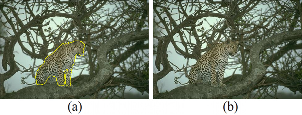
In this work, we coupled the sparse representation for image texture characteristics, dictionary construction, with the active contour evolution into a segmentation framework. Such framework has many nice properties: Firstly, one drops the a priori assumption for the texture model, such as MRF; Secondly, the capacity of the texture representation is only depending on the size of the dictionary and is theoretically unbounded. In addition to that, the segmentation (contour evolution) is actually performed on a scalar field, which significantly increases the efficiency. The basic idea/process is as follows: based on user’s initial drawing, two dictionaries for target and background are constructed. Such dictionary has the property that the representation of the texture of the image “patches” (to be defined in the next section) is sparse. Furthermore, an active contour is evolving in the image domain, and the advance or retreat of its front is based on the fitness of the local texture information with respect to either of the learned dictionaries. As a result, the texture analysis and the contour evolution are effectively coupled in the proposed Sparse Texture Active Contour (STAC) method, and a segmentation of the image is achieved. As a preview of the result, the segmentation result of one image is given in Figure 1. More detail of this case will be discussed in the Section III.

Fig. 1.

A preview for the result of the proposed segmentation method: (a) Original image. (b) Segmentation result.

The remainder of the paper is organized as follows. In Section II-A, we demonstrate the detail of how to construct the dictionaries for target and background. Then in Section II-B, the contour evolution is performed according to the learned dictionaries for the task of image segmentation. The experiments and results are performed in Section III. Finally, ongoing and future work is discussed in Section IV.

II. Method

In this section we present the details of the STAC algorithm. Specifically, the algorithm requires some brief user interactions. That is, the user is asked to provide some box region in both the foreground and the background. The algorithm then learns the texture of both foreground and background by constructing two over-complete dictionaries, which sparsely represent the textures in the image. The detail is given in the following section.

A. Texture dictionary

First, we denote the image to be segmented as a vector function I : Ω ⊂ ℝ² → ℝ^d, where d ∈ ℕ and usually d = 1 for grayscale images and d = 3 for RGB images. Furthermore, it is assumed that the user provides some drawings over the image indicating the foreground and background, which are denoted as a label map L : Ω ⊂ ℝ² → {0, 1, 2} where 1 indicates the target, 2 corresponds to regions in the background, and 0 (un-drawn region) means un-decided. As a result, such label map provides the information not only on where the target and nontarget regions are at, more importantly, how they look in this given image. Hence, in order to optimally exploit the available information, the segmentation algorithm ought to utilize both pieces of the information. Therefore, we first learn the image texture characteristics under the labeled pixels.

1) Patch bootstrapping

In order to learn the texture characteristics of the target, we collect “patches” from the target label regions. A target patch p is a sub-image of I confined in the target region. Formally, p : Δ ⊂ Ω → ℝ^d with p(x, y) = I(x, y) is a patch if and only if Δ ⊂ Ω and L(x, y) = 1 ∀(x, y) ∈ Δ. In this work, we restrict the patch domain, Δ, to a square containing k×k pixels. Next, N patches are extracted from the target region, as representatives for the target. Unfortunately, we then face the problem that, with a limited user-drawn area, many times there is not large enough space to accommodate N non-overlapping patches.

In this work, such problem is solved by making connection with the situation of performing statistical inference from limited samples [19]. Indeed, there the same difficulty lies in that the sample set is not large enough to infer the characteristics of the population with acceptable variance. In that case, the bootstrapping scheme [19] uses a sample-with-replacement strategy which successfully “enlarges” the sample set and reduces the estimation variance. In addition to that, the fact that the enlarged sample set has duplications inspires that the patches sampled form the user-drawn region in our situation do not have to be non-overlapping. With those observations, we perform the bootstrapping scheme to re-generate enough patches for our learning purpose. That is, a pair of random variables (x, y), is generated uniformly over Ω. If the region satisfies [x, x + k] × [y, y + k] ⊂ {(x, y) ∈ Ω : L(x, y) = 1}, this new patch p is then added to the patch list. This process is repeated until N patches are generated, and we denote the patch set as {p₁,…, p_N}. Finally, in order for the patches to be used in constructing the over-complete dictionary, each of them is re-written in a column vector by concatenating all its columns. We denote this process as q = p(:) ∈ ℝ^k2d and the patch list is Q = {q_i = p_i (:) ∈ ℝ^k2d; i = 1,…, N}.

2) Dictionary construction

Given the N elements in Q, a natural way to “learn” the information carried by them is to infer the underlying structure of the data. With the assumption that the underlying structure is a linear space, one constructs the basis from that. Moreover, if the elements are linear independent, the Gram-Schmidt process is one way to form the orthogonal basis. Similarly, the Karhunen-Loèeve transformation also constructs orthogonal basis minimizing the approximation error in l₂ sense. However, there are two unique features in the current situation that make the alternative method more desirable. First, the N elements in Q are not guaranteed to be linear independent. This is due to the fact that the patch size, k², is usually smaller than the total number of patches generated by the bootstrapping sampling. Secondly, the objective of constructing the basis (or dictionary) is such that the coefficients under the basis (or dictionary) is sparse in the l₀ norm. However, the aforementioned two schemes seeks minimizing the l₂ norm, which almost always gives non-sparse coefficients. In order to construct such over-complete dictionary, the K-SVD algorithm proposed by Aharon et al. is employed [2].

Formally, given the set of vectors {q₁,…, q_N} =: Q ∈ ℝ^k2d×N, the K-SVD algorithm seeks to find a full rank matrix F ∈ ℝ^k2d×M, called the “dictionary”, and the sparse coefficients γ_i’s:

$$\underset{F,\Gamma }{\text{min}}\Vert Q-F·\Gamma {\Vert }_F\mathrm{s}.\mathrm{t}.\Vert {\gamma }_i{\Vert }_0\le T$$ (1)

where the columns of the matrix Γ are the sparse coefficients γ₁,…, γ_N and ‖ · ‖_F indicates the matrix Frobenius norm. In order to be self-contained, we briefly reviewed the K-SVD method in Algorithm 1.

Algorithm 1.

K-SVD Dictionary Construction

1:	Initialize F
2:	repeat
3:	Find sparse coefficients Γ (γi’s) using any pursuit algorithm.
4:	for j = 1,…, M, update fj, the j-th column of F, by the following process do
5:	Find the group of vectors that use this atom: ζj := {i : 1 ≤ i ≤ M, γi(j) ≠ 0}
6:	Compute Ej := Q − ∑i≠j fi ${\mathrm{\Gamma }}_T^i$ where ${\Gamma }_T^i$ is the i-th row of Γ
7:	Extract the i-th columns in Ej, where i ∈ ζj, to form $E_j^R$
8:	Apply SVD to get $E_j^R$ = UΔV
9:	fj is updated with the first column of U
10:	The non-zeros elements in ${\Gamma }_T^i$ is updated with the first column of V × Δ(1, 1)
11:	end for
12:	until Convergence criteria is met

By minimizing the 0-norm of the coefficient we achieve the sparsity, which will benefit the computational burden of the subsequent contour evolution. After the convergence of the K-SVD algorithm, we denote the over-complete dictionary for the target patches as F := {f₁,…, f_M} where f_i ∈ ℝ^k2d and M is the number of atoms in the dictionary. Similarly, by applying the patch bootstrapping and dictionary construction for the background regions drawn by the user, we obtain the dictionary B ∈ ℝ^k2d×M for the background. The two dictionaries contain the image characteristics for the target and the background, and will be utilized in the subsequent contour evolution framework to extract the target from the image.

As an example, in Figure 2, we show the dictionary learned from the zebra region, and that from the background region, respectively.

Fig. 2.

The learning of texture dictionaries from an image. (a) The zebra image. (b) The dictionary learned from the zebra region. (c) The dictionary learned from the background, including sky and the grass, of the image.

B. Sparse Representation Driven Contour Evolution

After the foreground and background dictionaries having being constructed, we perform contour evolution to utilize the dictionary information and extract the target regions from the image. Intuitively, a dictionary is such that in it one can find an accurate enough approximation to a relevant item; and an erroneous approximation to an irrelevant item. With such intuition, we first compute the reconstruction error for the dictionary and a new image patch, to indicate how well the dictionary can represent the new patch under the sparsity requirement.

Formally, given a new image patch g : ℝ^k×k → ℝ^d, by slightly abuse of notation, we also consider g as a k × k × d dimensional array. Then, we compute the sparse coefficient η of g̃, defined as g̃ := g(:) ∈ ℝ^k2d×1, with respect to the dictionary F ∈ ℝ^k2d×M.

$$\underset{\mathit{\eta }}{\text{min}}\Vert \mathrm{g̃}-F·\mathit{\eta }{\Vert }_2\le \in \mathrm{s}.\mathrm{t}.\Vert \mathit{\eta }{\Vert }_0\le T$$ (2)

and the reconstruction error is denoted as

$$e_F:=\Vert \mathrm{g̃}-F·\mathit{\eta }{\Vert }_2$$ (3)

This problem is solved by the Orthogonal Matching Pursuit (OMP) method [46]. Similarly, the sparse coefficient ξ of g̃ under the dictionary B is also computed as:

$$\underset{\mathit{\xi }}{\text{min}}\Vert \mathrm{g̃}-B·\mathit{\xi }{\Vert }_2\le \in \mathrm{s}.\mathrm{t}.\Vert \mathit{\xi }{\Vert }_0\le T$$ (4)

and the reconstruction error is denoted as

$$e_B:=\Vert \mathrm{g̃}-B·\mathit{\xi }{\Vert }_2$$ (5)

Moreover, we define e := e_B − e_F. It is noted that the errors e_F and e_B indicate how well (or how bad) the new image patch can be reconstructed from information learned from the target and background region. Hence, the higher the e is, the more this patch is considered as the target region and vice versa. Furthermore, for each pixel (x, y) ∈ Ω, a patch p(x, y) is extracted as the sub-region of I defined on [x, x+k]×[y, y+ k]. Following the procedure above, we compute the e_F (x, y), e_B (x, y) and e(x, y) accordingly.

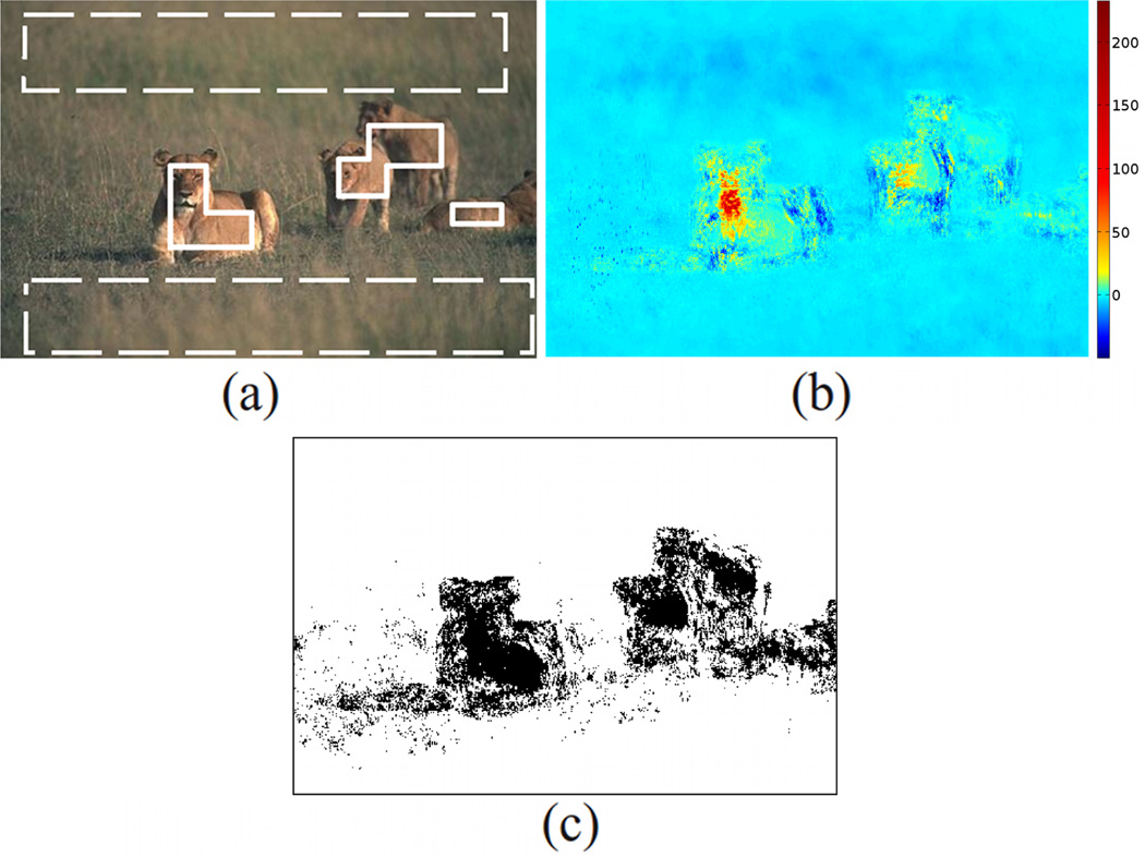
At the first sight, it might seem that this e(x, y) function, the error-difference image, would be enough for the classification. Indeed, we can just threshold the error-difference image by zero to obtain the classification. However, as shown in Figure 3, the error-difference image is very noisy and it is evident that the regularizer is necessary in drawing the final classification conclusion.

Fig. 3.

The image showing the necessity of using regularizer. (a) The initial boxes for target (solid) and background (dashed). (b) The error-difference image e (c) Binary image by thresholding the error-difference image with 0. We see the noisy nature of e and the necessity of regularizer in obtaining the final classification.

In this work, the active contour is used to group the information provided in the error-difference image in order to extract the target in the image. To this end, for a closed contour C : [0, 1] → Ω with C(0) = C(1), we define its energy E(C, I) as

$$E(C,I):=-(1-\lambda ){\int }_{(x,y)\text{inside}C}e(x,y)dxdy+\lambda {\int }_0^1\Vert \frac{dC}{dq}\Vert dq$$ (6)

where λ is the weight for the curvature regularizer. In order to evolve the contour to minimize the E(C, I), the artificial time variable is augmented such that C : [0, 1]×[0, +∞] → Ω, with C(0, t) = C(1, t), ∀t. Moreover, denote the user specified target region as Ω_T := {(x, y) ∈ Ω, L(x, y) = 1}. The initial position of the contour is assigned as ∂Ω_T. Furthermore, the first variation of the energy is computed and the flow of the contour can be written as:

$$\{\begin{array}{c}\frac{\partial C}{\partial t}:=-{\nabla }_{C}E(C,I)=(1-\lambda )e(C(q))\mathit{N}(q)-\lambda \kappa (q)\mathit{N}(q)\hfill \\ C(q,0)=\partial {\mathrm{\Omega }}_T\hfill \end{array}$$ (7)

where N(q) is the unit normal of C(q). The contour evolves according to the flow defined in equation (7) and its position at convergence indicates the final segmentation.

Looking back to our discussion on how to maximally utilize the user provided initial information in Section II-A, we see that many of the previous active contour based method only utilizes the user seeds as the initial contour position, but did not take advantage of the image information under the seeds to characterize the target. Instead, various pre-defined models are used to define the target. Similarly, many graph based segmentation methods better utilize the position of the background seeds, and effectively reject the final target contour intruding into those region. Still, the weight assignment on the graph is only related with the pre-defined edge model, such as high gradient magnitude. Contrastingly, in this work the STAC makes use of both the foreground and background seed regions, in a manner that the textures are learned and drives the contour evolution, which is initiated from the target region. Therefore, from the theoretical point of view, the proposed method maximally utilizes the user provide information and is expected to give satisfiable results, which we will present in the following experiment section.

III. Experiments and results

In this section we first show the segmentation of eight specific cases and analyze the segmentation process, user interaction and result in detail. Then, we perform the segmentation on the images provided in [24] and present the quantitative statistical analysis. Finally, we provide cases where the performance is not high, which lead to the possible future directions.

A. Natural images with user interactivity analysis

In this section we performed the segmentation using the proposed STAC algorithm on several images from the Berkeley Image Dataset [41], [42]. Each of these images is selected to represent a certain category of texture and/or target shape. In each experiment, we compared the STAC with other textural image segmentation schemes such as: active contour using Gabor filtering [53], regional statistics (CV) [8], [9], the weighted curve evolution using modulation features [29]. Moreover, some interactive segmentation methods which are not necessarily using texture information are also included in the comparison, such as the Lazysnap [33] and [49]. As usual, an user driven algorithm depends on the way user initializes the algorithm. Because of that, in this sub-sections we give some rather explicit details on the user interaction and thus they have both an experimentation and a tutorial flavors.

In order to achieve a consistent comparison, when applicable, we used the same initialization for each of the methods being tested. This, however, may not be the optimal initialization for some of the methods compared. Indeed, it is true that with more specific tuning (which will be discussed for each case), most of the interactive methods will provide better results which eventually converge to the human ground truth as the input increases. Therefore, it should be emphasized that the purpose of such comparison is not to claim the STAC be superior to any existing techniques, but provides a promising new alternative approach to the texture image segmentation task.

As for the parameters of the proposed method, we fixed M = 300 for the dictionary size defined in Section II-A1. For the Gabor wavelet based active contour [53], we adopted the choices suggested by the original paper (with the same parameter names there): θ ∈ {0, π/6, π/4, π/3, π/2}, F ∈ {60, 90, 120}, and σ ∈ {0.0075, 0.005, 0.0025}. The active contour always evolves to the convergence. Moreover, for the lazysnap method, the result obtained by the watershed pre-processing, followed by the graph cut segmentation is considered to be the final output here; That is, the further intelligent boundary manual editing is not pursued.

Moreover, the contours in the figures of this section are with various colors. Those colors are chosen so that they have high contrast for both screen viewing and grayscale print.

1) Zebra

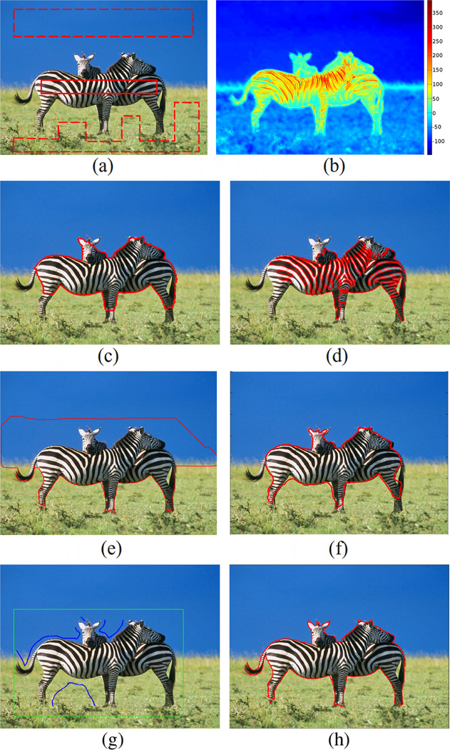
Zebra images may be the most frequent choice for the texture image processing techniques. Therefore, the algorithm is first tested on a Zebra image shown in Figure 4(a). For human visual perception, the scene of this image is not very complicated to be decomposed. However, the region based active contour (for scalar image), starting from the solid box position in Figure 4(a), is not able to extract the correct object from the image. Instead, it segments the darkest colored regions in the image and gives the results in Figure 4(d). This is because the texture of the target consists of very inhomogeneous texture pattern (black and white), but the method uses the pre-defined target model that the mean intensity being different from the background. It is noted that this is the only appearance of directly applying the vector image region based active contour, and it’s only to confirm the necessity of using the texture. Indeed, with Gabor wavelet based texture segmentation method in [53], a nice result can be achieved. However, due to the space constraint, its result is not shown here but in the other experiments.

Fig. 4.

Zebra image. (a) The initial boxes for target and background (b) Error-difference image (c) Result by Lazysnap (d) Result by Vector valued CV (e) Result by GrabCut (f) STAC (g) The seeds (green: target bounding box; blue: background) for the grabCut in order to obtain the result in (h).

As a comparison, using the solid box as the target seeds and the dashed box as the background seeds, we performed the graph based lazysnap algorithm whose result is shown in Figure 4(c). In addition, the result of the GrabCut is given in Figure 4(e). Due to the seeds of the sky being higher than what is preferred by the GrabCut algorithm, the upper region is not well segmented under such initialization. Finally, the STAC is performed. It first learns the target (background) texture from the solid (dashed) box, respectively, and then drives the contour to convergence. The result is shown in Figure 4(f). In this test, this result is not much different from that of the lazysnap, except the fact that the STAC captures more of the lower leg. Moreover, it can be observed that since the solid box in the learning stage does not contain the tail, and the texture of the tail differs from that of the body, the final result does not contain the tail either.

2) Fish

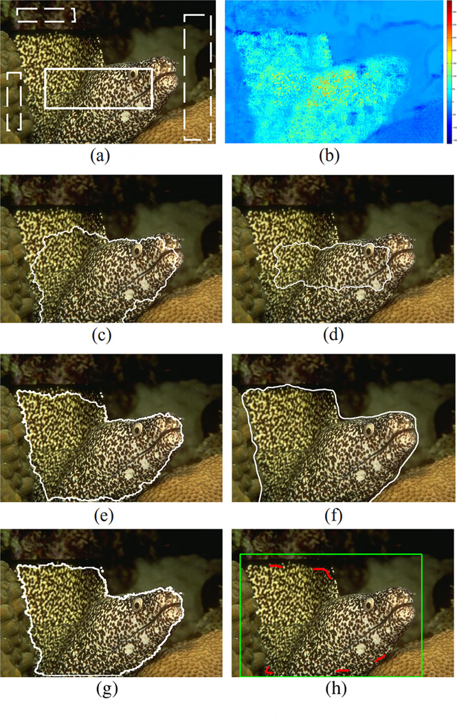
For the fish data set, with the same initial labels show in Figure 5(a), the proposed method more accurately captures the target. However, it is also noted that with more detailed seed labels in the top part of its fin and head, and more background labels above its head, the lazysnap is able to capture the fish correctly. The Gabor texture based active contour [53] result is not very far from the initial position. This may be due to the fact that the texture contents inside and outside the contour are similar, preventing the contour from evolving and making it converge too early. The GrabCut gives a good result also, with just two corners in the top-middle and bottom-left regions missing. This may because the image brightness of those places are darker and more similar to that of the background. Putting more target seeds in those regions may solve the problem. On the other hand, the STAC utilizes the texture information and correctly gives the right segmentation.

Fig. 5.

Fish image. (a) The initial boxes for target and background (b) Errordifference image (c) Result by Lazysnap (d) Result by [53] (e) Result by GrabCut (f) STAC (g) The seeds (green: target bounding box; red: target) for the grabCut in order to obtain the result in (h).

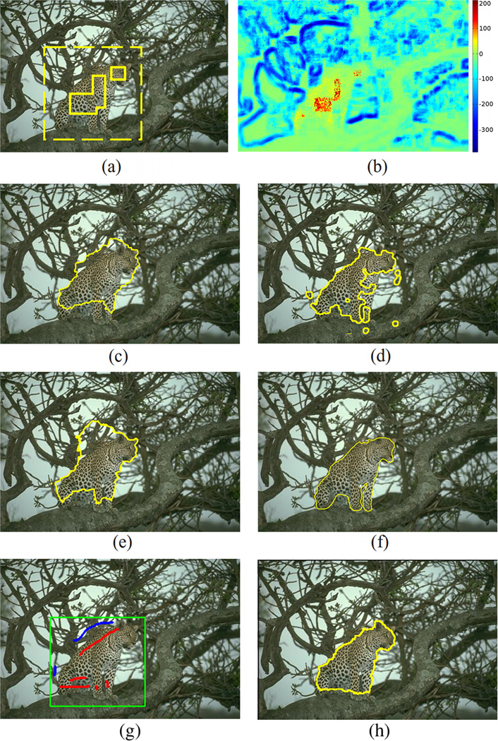
3) Snow leopard

Even for human eyes, the snow leopard in Figure6 is rather difficult to segment. Indeed, here we need to use everything outside the dashed white box to learn the background texture. However, in the step of contour evolution after texture learning, there is no explicit constraint preventing the contour from growing out of the dashed box (for STAC). Nevertheless, with the learned texture information, the STAC correctly extracts the target, only missing its right leg. On the other hand, in our test, without the initial seeds being close to the true segmentation, the graph based algorithm was not able to find the correct boundary. This may partially due to the fact that the graph based algorithm uses the image gradient to assign the edge weight, but the image gradient is rather low between the leopard body and the tree branches. In such a situation, the texture framework is the key in finding the proper edge between the target and the background. In addition, the method in [29] captures most of the leopard region. However, that method is unsupervised so it is more difficult to separate the target from the background, some regions of which having very similar texture to the leopard even for the human eyes. Hence, to mitigate such effect, a post processing is added which performs an XOR operation between the direct algorithm output with the manually given background region, and the final result is shown in Figure 6(d). With more target seeds in the lion’s back and more background seeds in the tree/sky nearby, the GrabCut would give better results.

Fig. 6.

Snow leopard image. (a) The initial boxes for target and background (b) Error-difference image (c) Result by Lazysnap (d) Result by [29] (e) Result by GrabCut (f) STAC (g) The seeds (green: target bounding box; blue: background; red: target) for the grabCut in order to obtain the result in (h).

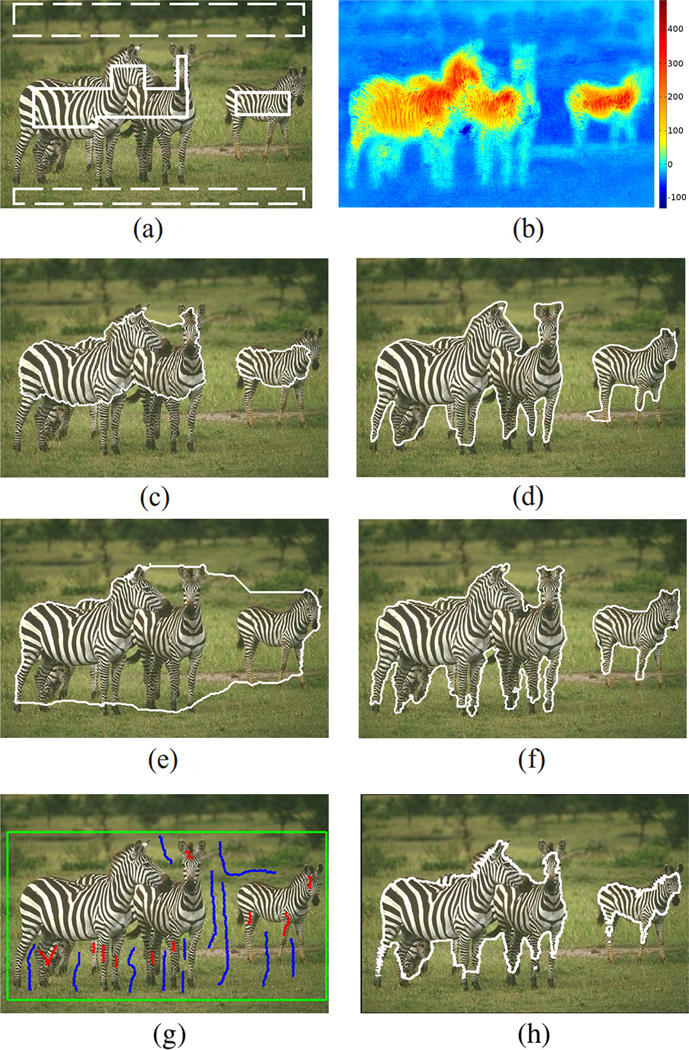
4) Three zebras

This zebra image is more difficult than the one in Section III-A1 and the performances here are not as good as that one. Indeed, here the background is not purely blue sky and green grass but having similar colors to the target. Given such a situation, the proposed method gets better results in particular in those concave regions such as the region between the heads of the two zebras. For the graph based method, it can be seen that the final contour fails to capture most of the legs. This is because the method is still based on the image gradient, but being different from the low gradient as in the leopard case, here the gradient is almost high everywhere. Therefore, a common behavior of the contour is just stopping at some high gradient position roughly in the middle of the target seeds and the background seeds. As a comparison, the Gabor wavelet based texture segmentation method in [53] gives the result of Figure 7(d). It can be seen that except for few regions, the performance is satisfying. Finally, our STAC method gives the result shown in Figure 7(b). While most of the target is well captured, it still misses the left leg of the right-most zebra.

Fig. 7.

Zebra image. (a) The initial boxes for target and background (b) Error-difference image (c) Result by Lazysnap (d) Result by [53] (e) Result by GrabCut (f) STAC (g) The seeds (green: target bounding box; blue: background; red: target) for grabCut in order to get the result in (h).

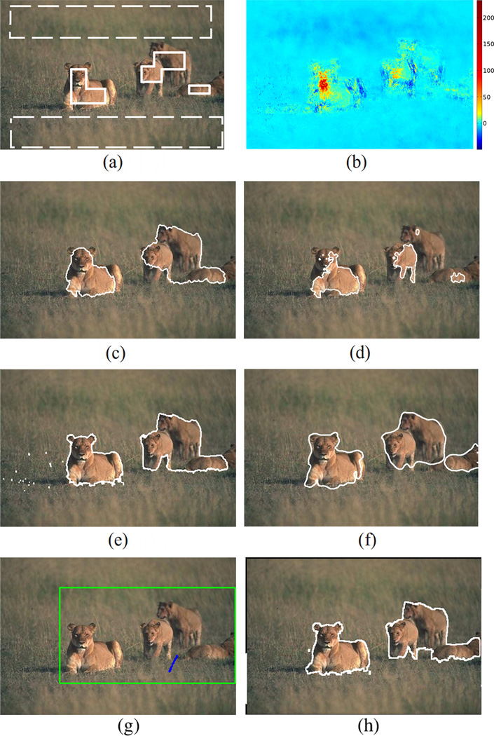
5) Lions

The image in this test is chosen because it is of a similar type to the previous one, but its background and foreground are even more difficult to differentiate, as a consequence of that the foreground and the background share very similar color. However, the grass background has certain texture pattern which is captured by the STAC and a nice result is obtained. The modulation feature based method in [29] gives the result in Figure 8(c), and the Gabor wavelet based regional active contour gives Figure 8(d), which misses certain low brightness regions. The GrabCut gives nice segmentation in this case (Figure 8(e)), especially at the front leg of the first little lion.

Fig. 8.

Lion image. (a) The initial boxes for target and background (b) Error-difference image (c) Result by [29] (d) Result by [53] (e) Result by GrabCut (f) STAC (g) The seeds (green: target bounding box; blue: background) for grabCut in order to get the result in (h). It is noted that (b) has been shown in Figure 3 and is shown again for completeness.

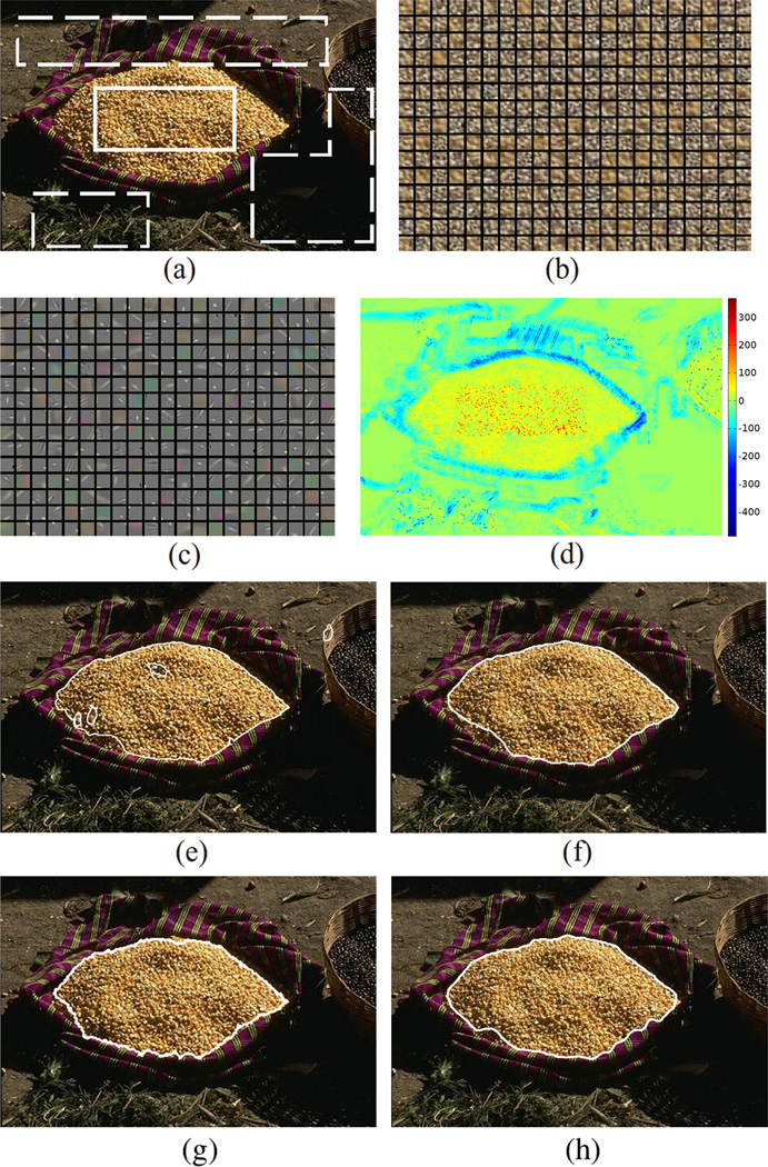
6) Beans in the bag

This image was chosen in order to demonstrate the “backward compatibility” of the proposed method. Indeed, this bean image is not difficult for our vision system, and if one designs an algorithm to extract certain color content from the image, with certain smoothness constraint, it is very likely to obtain a good results for this particular image. By trial and error, we find that the Cb component (blue-difference chroma component) of the YCbCr color space is a suitable choice [5]. Indeed, in the Cb image, using the scalar region based active contour in [9] gives the result shown in Figure 9(f). Nevertheless, such choice is not generalizable to handle the other cases.

Fig. 9.

Bean image. (a) The initial boxes for target and background (b) Dictionary for the target (c) Dictionary for the background (d) Error-difference image (e) Result by [29] (f) Result by Scalar valued CV in Cb component image in the YCbCr color space (g) Result by GrabCut (h) STAC

The method proposed in [29] is also tested and the result, in Figure 9(e), is consistent with one shown in the original paper. It can be observed that some darker region of the beans are not included in the output contour. Moreover, a piece of background is considered to be the target.

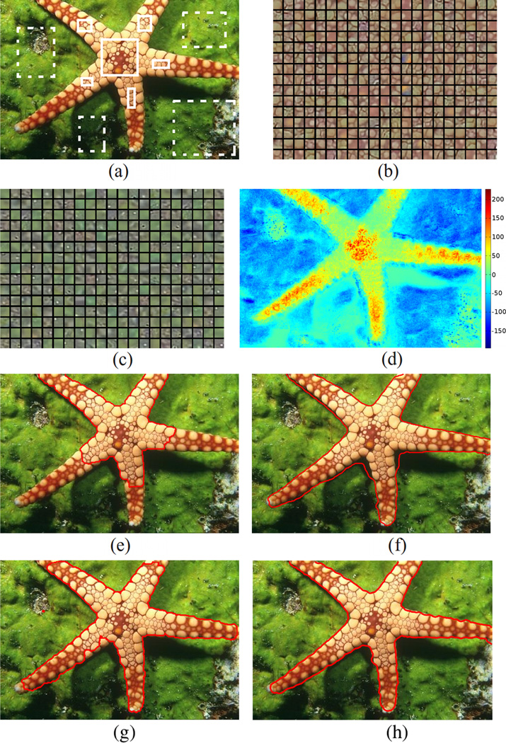
7) Sea star

This testing image shares similar property as the previous one in that it seems to be easy to segment by using the color information. Again by some testing, we found that the hue component of the HSV color space is suitable for this case [5]. Consequently, using the scalar Chan Vese active contour, we get the result in Figure 10(e).

Fig. 10.

Sea star image. (a) The initial boxes for target and background (b) Dictionary for the target (c) Dictionary for the background (d) Error-difference image (e) Result by Lazysnap (f) Result by Scalar valued CV in the hue component image in HSV color space (g) Result by GrabCut (h) STAC

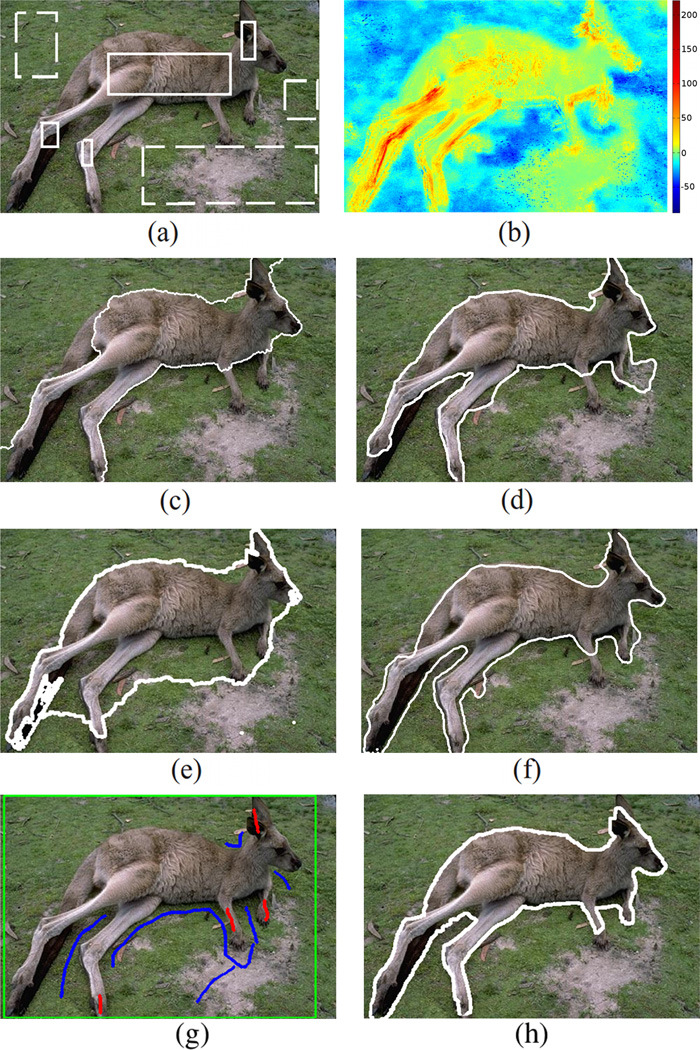
For the graph based method, however, the high gradients of the texture stop the propagation of the foreground region in the middle of its three legs. Indeed, it has already been observed in Figures 4(c), 6(c), and 7(c), that the graph based method usually performs not so well for the long narrow structures such as legs, in particular in these textural images. In fact, theoretically, it many times is less expensive to cut the graph by directly connecting the tips of the two legs, even if such path has a higher average weight (per edge). On the contrary, if the cut goes along the leg, although the average weight is smaller, the longer total distance is more likely to make such choice less probable. In such situations, one often needs fine tune the method by drawing extra background seeds in the regions between the narrow structures, and also more foreground seeds roughly following the center line of the narrow structures. Such work needs to be done with care in the narrow area and is usually more time consuming than drawing the boxes shown in Figure 11(a). It is noted that such long narrow structure also posses difficulty for the active contour based algorithms. For example, it has been studied in [60], and specially treated for tubular structure in [44]. However, in this work, without those special treatment, the problem is solved quite satisfyingly.

Fig. 11.

Kangaroo image. (a) The initial boxes for target and background (b) Error-difference image (c) Result by Lazysnap (d) Result by [53] (e) Result by GrabCut (f) STAC (g) The seeds (green: target bounding box; blue: background; red: target) for the grabCut in order to obtain the result in (h).

8) Kangaroo

This image is selected for two reasons: First, we would evaluate how the algorithm performs on more difficult long narrow structures, i.e., the arms and the legs of the kangaroo. For this purpose, we see that the STAC correctly differentiate the two legs and the grass in between. However, especially for the right arm, the algorithm did not perform very well.

In addition to that, the second purpose is to evaluate the capability of the STAC in handling the situation where the foreground has larger color/texture/lumination variation than the background. Indeed, in many segmentation tasks, because the background contains “everything else”, it thus has larger photometric variation, and the target is usually of relative smaller change. Such situation is in fact of benefit to the segmentation process because usually the segmentation is driven by a pre-defined photometric model of the target. Therefore, the simpler the target is, the easier it is to be modeled. However, the image here does not fall into such category. Indeed, the background is rather monotonous with green grass and a few earth whereas the foreground has large intensity ranging from very dark (on the tail and the ear) to very bright (on the legs). Nevertheless, the proposed method is symmetric over the foreground and the background, hence it does not rely on the assumption that the foreground having less richer content than the background. As a result, such capability is reflected in the successful segmentation in Figure 11(b).

B. Statistically analysis and choices for parameters

For reproducibility, the parameters used for the experiments in Section III-A are summarized in Table I. Furthermore, the quality of segmentation was further quantitatively measured by the Dice coefficient [14]. For the two sets,Ω ₁ and Ω₂ representing two extracted regions, the Dice coefficient between them is defined as:

$$s:=\frac{2|{\mathrm{\Omega }}_1\cap {\mathrm{\Omega }}_2|}{|{\mathrm{\Omega }}_1|+|{\mathrm{\Omega }}_2|}$$ (8)

The Dice coefficient is in the range of [0, 1] and the closer it is to 1, the similar the two sets Ω₁ and Ω₂ are.

TABLE I.

Parameters used for each experiment. For the STAC, the Sparsity is the T defined in Equation (2), and the k is the patch size. Moreover, for the scalar Chan Vese method, the Length weight is the μ term of Equation (9) in [9] (with ν = 0), and similarly for the Length weight of the Gabor wavelet based method in [53]. Lastly, the λ is defined in Equation (54) in [29].

Image name	STAC		Chan Vese [9]	Gabor [53]	AM-FM [29]
	Sparsity	k	μ in [9]	μ	λ in Eq.(54) in [29]
Zebra	8	12	—	—	—
Fish	8	18	—	2	—
Snow leopard	12	10	—	0.5	0.9
Three Zebras	12	10	—	1	—
Lions	15	10	—	1	0.8
Beans in the bag	8	8	2	—	0.8
Sea star	8	12	2	—	—
Kangaroo	15	12	—	2	—

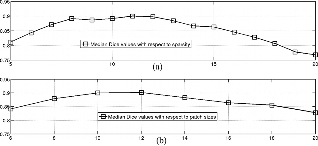
Subsequently, in order to investigate how the parameter T (defined in Equation (2)) affects the result, different values of it are tested and the results are compared with the human ground truth provided in [42] by computing the Dice coefficients. The results are shown in Figure 12. It can be seen that T being too larger or too small both reduce the segmentation accuracy. Indeed, with a larger T, the representation capability increases for both dictionaries. As a result, in the case where the textures of the target and the background are similar, the error of reconstructing the target using the background dictionary would not be so poor and vice versa. Hence, the strong contrast in the error-difference image is not evident and the final segmentation accuracy decreases. On the other hand, when T is too small, neither dictionary is able to get a good enough representation for the texture of its kind. This also leads to a sub-optimal discriminating ability.

Fig. 12.

Dice coefficient by varying the sparsity. The horizontal axis shows the sparsity used in the K-SVD and OMP. The vertical axis is the Dice coefficient.

In addition to the sparsity term T, the texture representation capability is also affected by the size of the patch. A too small patch would not be able to capture the textual information in the target/background because texture by its nature is some pattern that repeats. However, if the patch is too large, it may also include non-representative textual information. This is especially evident at the boundary region. Hence, In order to quantify that effect, we vary the patch size and perform the segmentation to measure the corresponding change in the Dice coefficient, as shown in Figure 13.

Fig. 13.

Dice coefficient (vertical axis) by varying the patch size (horizontal axis).

Furthermore, the above analysis is applied on all the test images in [42], and the median dice coefficients are plotted in Figure 14.

Fig. 14.

The Median Dice coefficients for all the testing images. (a) Median Dice coefficients with different sparsity. (b) Median Dice coefficients with different patch size.

The median, instead of the mean, is used in the previous case because there exist some outlier cases where the algorithm does not perform very well. Those cases will be detailed in the next section.

C. Quantitative evaluation

In order to further quantitatively evaluate the algorithm on larger variety of images, we conduct the following experiments. The data set containing a total of 151 images is used [24]. In order to perform consistent comparisons for the interactive methods which are designed to take advantage of the flexibility of the user inputs, we utilize the segmentation ground truth provided in [24]. More explicitly, for each testing image I : Ω ⊂ ℝ² → ℝ^d and its ground truth binary segmentation result T : Ω → {0, 1} where 1 indicates inside the target and 0 means background, we first compute the areas of the target and background as A_t and A_b, respectively. Then, a signed distance image τ : Ω → ℝ is constructed from T as:

$$\tau (\mathit{x})=\{\begin{array}{cc}-{\text{min}}_{\mathit{y}\in \partial T}\Vert \mathit{x}-\mathit{y}{\Vert }_2\hfill & \text{if}T(\mathit{x})=1\hfill \\ {\text{min}}_{\mathit{y}\in \partial T}\Vert \mathit{x}-\mathit{y}{\Vert }_2\hfill & \text{if}T(\mathit{x})=0\hfill \end{array}$$ (9)

where ∂T ⊂ Ω is the boundary of the target region and ‖ · ‖₂ denotes the Euclidean norm. Then, two levels V_t and V_b are chosen such that:

$$|\{\mathit{x}\in \mathrm{\Omega }|\tau (\mathit{x})\le V_t\}|=A_t/2$$ (10)

$$|\{\mathit{x}\in \mathrm{\Omega }|\tau (\mathit{x})\ge V_b\}|=A_b/2$$ (11)

After that, the label image L(x) is defined as:

$$L(\mathit{x})=\{\begin{array}{cc}1\hfill & \text{if}\tau (\mathit{x})\le V_t\hfill \\ 2\hfill & \text{if}\tau (\mathit{x})\ge V_b\hfill \\ 0\hfill & \text{otherwise}\hfill \end{array}$$ (12)

This label image, together with the original image I(x), are input to each of the algorithms for comparison. It is noted that the construction of such input label image is for the purpose of consistency across the different algorithms being tested. As a result, it may not be optimal for the segmentation results. The average and standard deviation of the Dice coefficients for all the 151 images are shown in Table II.

TABLE II.

Mean and standard deviation of the Dice values of groups the 151 testing images for the methods compared. It can be observed that the proposed STAC method has the highest Dice value among them. In addition to that, STAC has a much smgroupser variance for groups the testing images demonstrating the robustness of the method in the difficult images.

	Lazysnap	GrabCut	Gabor Texture	AM-FM	STAC
Mean	83.6%	88.2%	77.3%	82.1%	88.5%
Std-dev	7.21%	7.37%	6.19%	5.81%	3.77%

From Table II we can observe that the proposed STAC method has the highest Dice value among the methods being compared. In addition to that, STAC has a much smaller variance for all the testing images. In addition, for those testing images with strong texture, the methods with texture modeling in their design (Gabor Texture, AM-FM, and STAC) in general outperform those algorithms that are faster but do not consider texture feature. This is shown as the differences in the Dice value standard deviations in Table II. Due to the fact that the input label images are not optimized for any of the methods being compared, the Dice values are in general not as high as those reported in their respective original papers.

D. Initialization sensitivity evaluation

Good initialization is necessary for achieving good final segmentation. In this section, we vary the initial input for those cases where good segmentations have been achieved, and quantitatively measure how much the results changes/degrade with respect to the degradation of the initial input. Among the 151 images tested, 39 of them achieved a Dice score above 0.9, which are considered here as good. Then, their initial foreground/background masks are shrunk. With less learning pattern, the results usually get worse. In order to measure this process quantitatively, we conduct the following experiments. For each input label image L(x) defined in Equation (12), two signed distance images τ_f and τ_b are defined, respectively for the initial foreground and background regions, according to Equation (9). The initial foreground region is shrunk by binarilizing τ_f at threshold α_f < 0. As α_f decreases, the region {x|τ_f (x) ≤ α_f} is also reduced. Until such region is unable to enclose a single k × k pixel square patch, we denote the corresponding threshold to be ${\alpha }_f^{*}$. Similarly for the background region, the critical threshold is denoted as ${\alpha }_b^{*}$. Then, a series of label images L_i (x) : i = 0,…, 9 are constructed as:

$$L_i(\mathit{x})=\{\begin{array}{cc}1\hfill & \text{if}{\tau }_f(\mathit{x})\le i·{\alpha }_f^{*}\hfill \\ 2\hfill & \text{if}{\tau }_b(\mathit{x})\le i·{\alpha }_b^{*}\hfill \\ 0\hfill & \text{otherwise}\hfill \end{array}$$ (13)

Note that L₀ coincides with L in Equation (12). After that, each of the 10 label images L_i is used to initialize the segmentation and the resulting Dice values are recorded. Such experiment is repeated for all the 39 images and their results are given in Table III.

TABLE III.

Mean and standard deviation of the Dice values of groups the 39 testing images with shrinking input label images. This demonstrates the algorithm performance with respect to worse and worse initialization.

i in Equation (13)	0	1	2	3	4	5	6	7	8	9
Mean	90.6%	88.1%	86.8%	79.1%	66.9%	53.4%	55.4%	47.7%	32.1%	21.8%
Std-dev	7.11%	13.8%	16.3%	16.1%	20.6%	28.2%	27.1%	22.5%	18.3%	11.2%

In general, shrinking from the “good” initial label masks which result in Dice values greater than 90%, the resulting Dice values drop slowly for approximately the initial 20% of the process (i < 3). After that the performances degrade quickly. This test is also performed to GrabCut, Gabor Texture, and AM-FM methods. For each i, the resulting 39 Dice values of each of the three methods are compared with those from the proposed STAC algorithm using a one sided t-test. At a p-value of 0.05, the hypothesis that STAC perform equally or worse, is reject. Referring to the second row of Table II that STAC gives smaller standard deviation in Dice values, this experiment demonstrates again that the proposed algorithm is more robust to the large variation of different image types.

E. Active contour regularized clustering

We further compare the proposed algorithm with different clustering algorithm regularized by the active contour method. Initially, four clustering algorithms had been considered: K-means, normalized cut [55], mean shift [11], and affinity-propagation [21]. The idea is to use the various clustering algorithms to perform an initial classification, and then use active contour to regularize the resulting boundary between the foreground and background. However, one of the features of the mean shift and the affinity-propagation algorithms is that the number of clusters is not required to be known a priori. Such flexibility, on the other hand, makes the subsequent active contour regularization a difficult task. Because we are focusing on the bi-segmentation cases and it is not clear how the multi-region active contour is to be applied to such cases. As a results, the K-means and the normalized cut (NCUT) algorithms are picked due to their ability to fix the number of clusters a priori.

For the K-means, two experiments have been conducted. First, the feature vector at each pixel is simply the d-dimensional image values vector. In order to reduce the local minima problem in K-mean clustering, multiple (10³) trials are performed. In each trial, the initial class centers are picked at random in their respective label regions. The purpose of such configuration is to test the algorithm without incorporating the local neighbor textural information. In the second experiment setup, for each pixel, the feature is a k²d-dimensional q vector as defined in Section II-A where the image value at the k × k neighboring pixels are all concatenated as a single vector. After the K-means clustering, similar to the proposed STAC algorithm, at location (x, y) the error value e(x, y) as in Equation (6) is computed as the e_B − e_F where e_B is the distance from the feature vector at this location to the centroid of the background class, and e_F is the distance from the current feature vector to the centroid of the foreground class. Such error image then drives the active contour evolution which gives the final segmentation.

For the NCUT algorithm, two similar experiments have also been conducted, differed only by the assignment of graph weights. That is, following [55], the image values is used in the first experiment. While in the second test, the k²d-dimensional feature vector q as defined in Section II-A is used to compute the weights on the graph. After the generalized eigen-decomposition, the active contour regularization is carried out by performing the standard Chan-Vese segmentation on the image form by the eigen vector corresponding to the second-largest eigen value.

As shown in Table IV, those experiments utilizing the neighboring texture information result in higher Dice values. This again demonstrated the necessity of incorporating the textural information in the segmentation process.

TABLE IV.

Mean and standard deviation of the Dice values of groups the testing images with “clustering + active contour”.

Dice	K-means, 1st	K-means, 2nd	NCUT, 1st	NCUT, 2nd
Mean	62.7%	77.0%	70.9%	79.1%
Std-dev	9.88%	8.54%	8.15%	7.47%

F. Cases not working well

The algorithm starts with the user drawn box regions from which the texture is learned. However, for certain target whose shape is narrow and curved, the box is not easy to draw. As a result, the learning of the texture is affected and the subsequent segmentation performance is impaired. One of such case is given in Figure 15. From that we can see the curved and narrow shape of the snake makes the initial box difficult to be put, as a result, the final segmentation is not well.

Fig. 15.

Due to the difficulty in giving the initial region for learning the texture, the segmentation performance is not well for this case. (a) The original image with user initial boxes for target (solid) and background (dashed). (b) The error-difference image. (c) Segmentation result.

In such cases, those interactive segmentation schemes where the dots or strokes are used as user input (or editing tool), for example in [3], [54], [58], [33], [49], may have more advantage and better performance.

IV. Conclusion and Future Work

In this work, we present a method to characterize the image texture utilizing the sparse representation theory, and the usage of texture information in driving the active contour evolution to perform the image segmentation tasks. In short, the user is asked to draw a few boxes in the fore/background in the image and the texture dictionaries are constructed to sparsely represent the characteristics within and out of the target. Then, an active contour is evolved to optimize the fidelity of the representation provided by the dictionary of the target. The algorithm is then tested on several representative images and compared with other well known methods, to demonstrate the capability of the proposed algorithm in handling very challenging images.

Future work will include extending the algorithm to higher dimension and wider image types. In particular, most of the medical images are in 3D or even higher dimension, and the texture provides much information about the health/pathology condition of the subject. Therefore, the proposed method may provide good tools for the segmentation and classification in the medical image analysis field.

Moreover, it is noticed that in [37] the dictionaries are learned by not only considering the textures belonging to the current group but also the other groups. Doing this will improve the discriminative capability of the dictionary and leading to better segmentation. Furthermore, our method may be extended to extract multiple objects by employing the Potts model [7].

Currently, when user input is updated, the entire dictionary is learned again and this is a time consuming step. It is noted that several incremental dictionary construction researches have shown a very promising direction for performance improvement [63], [40], [30]. Although the main objective of this work is to demonstrate that coupling the two powerful tools, active contour and sparse representation, into a common framework is a promising technique for texture image analysis, we will further pursue in this incremental learning direction to improve the time performance of the segmentation algorithm.

In addition to the improvement on the methodology, better user interface can be constructed so that the initial regions can be drawn by user with better flexibility, instead of boxes as in the current form. This will lead to the solution for the cases discussed in Section III-F.

Biographies

Yi Gao graduated with a PhD degree at the Georgia Institute of Technology. Currently, he is a research fellow in the Psychiatry Neuroimaging Laboratory, Harvard Medical School. His research interests include image and shape computing.

Sylvain Bouix is an Assistant Professor and Associate Director, Psychiatry Neuroimaging Laboratory, Department of Psychiatry, Brigham and Women’s Hospital, Harvard Medical School. He received his B.Eng. from Institut Polytechnique de Sevenans, France his M.Sc. from the University of Kansas and his Ph.D. from McGill University. His research interests include shape analysis of anatomical structures and evaluation of medical imaging techniques. His main duty is to act as a mediator between computer scientists and neuroscientists to help improve computer tools for neuroimaging studies. Martha E. Shenton is Professor in the Departments of Psychiatry and Radiology, Brigham and Women’s Hospital, Harvard Medical School, and a Health Scientist at the VA Boston Healthcare System. Her research interests include applying sophisticated image processing techniques to understand neuropsychiatric disorders.

Martha E. Shenton is Professor in the Departments of Psychiatry and Radiology, Brigham and Women’s Hospital, Harvard Medical School, and a Health Scientist at the VA Boston Healthcare System. Her research interests include applying sophisticated image processing techniques to understand neuropsychiatric disorders.

Allen Tannenbaum is a faculty member in the School of Electrical and Computer Engineering at Boston University. His research interests include systems and control, computer vision, and image processing. He is a fellow of the IEEE.

References

- 1.Adam A, Kimmel R, Rivlin E. On scene segmentation and histograms-based curve evolution. IEEE Transactions on Pattern Analysis and Machine Intelligence. 2009;31:1708–1714. doi: 10.1109/TPAMI.2009.21. [DOI] [PubMed] [Google Scholar]
- 2.Aharon M, Elad M, Bruckstein A. K-SVD: An algorithm for designing overcomplete dictionaries for sparse representation. IEEE Transactions on Signal Processing. 2006;54:4311. [Google Scholar]
- 3.ArbelÁez P, Maire M, Fowlkes C, Malik J. Contour detection and hierarchical image segmentation. IEEE transactions on pattern analysis and machine intelligence. 2010:898–916. doi: 10.1109/TPAMI.2010.161. [DOI] [PubMed] [Google Scholar]
- 4.Bovik A, Clark M, Geisler W. Multichannel texture analysis using localized spatial filters. IEEE Transactions on Pattern Analysis and Machine Intelligence. 1990:55. [Google Scholar]
- 5.Burger W, Burge M. Digital image processing: an algorithmic introduction using Java. Springer-Verlag New York Inc; 2008. [Google Scholar]
- 6.Caselles V, Kimmel R, Sapiro G. Geodesic active contours. International Journal of Computer Vision. 1997;22:61. [Google Scholar]
- 7.Celeux G, Forbes F, Peyrard N. Em procedures using mean field-like approximations for markov model-based image segmentation. Pattern recognition. 2003;36:131–144. [Google Scholar]
- 8.Chan T, Sandberg B, Vese L. Active Contours without Edges for Vector-Valued Images. Journal of Visual Communication and Image Representation. 2000;11:130. [Google Scholar]
- 9.Chan T, Vese L. Active contours without edges. IEEE Transactions on Image Processing. 2001;10:266. doi: 10.1109/83.902291. [DOI] [PubMed] [Google Scholar]
- 10.Chang T, Kuo C. Texture analysis and classification with tree-structured wavelet transform. IEEE Transactions on Image Processing. 1993;2 doi: 10.1109/83.242353. [DOI] [PubMed] [Google Scholar]
- 11.Comaniciu D, Meer P. Mean shift: A robust approach toward feature space analysis. IEEE Transactions on Pattern Analysis and Machine Intelligence. 2002;24:603–619. [Google Scholar]
- 12.Cong Z, Xiaogang W, Wai-Kuen C. Background subtraction via robust dictionary learning. EURASIP Journal on Image and Video Processing. 2011;2011 [Google Scholar]
- 13.Cross G, Jain A. Markov random field texture models. IEEE Transactions on Pattern Analysis and Machine Intelligence. 1983;5:25. doi: 10.1109/tpami.1983.4767341. [DOI] [PubMed] [Google Scholar]
- 14.Dice L. Measures of the amount of ecologic association between species. Ecology. 1945;26:297–302. [Google Scholar]
- 15.Donoho D. Compressed sensing. IEEE Transactions on Information Theory. 2006;52:1289. [Google Scholar]
- 16.Donoho D, Elad M. Optimally sparse representation in general (nonorthogonal) dictionaries via L1 minimization. Proceedings of the National Academy of Sciences. 2003;100:2197. doi: 10.1073/pnas.0437847100. [DOI] [PMC free article] [PubMed] [Google Scholar]
- 17.Dunn D, Higgins W. Optimal Gabor filters for texture segmentation. IEEE Transactions on Image Processing. 1995;4:947. doi: 10.1109/83.392336. [DOI] [PubMed] [Google Scholar]
- 18.Dunn D, Higgins W, Wakeley J. Texture segmentation using 2-D Gabor elementary functions. IEEE Transactions on Pattern Analysis and Machine Intelligence. 1994:130. [Google Scholar]
- 19.Efron B, Tibshirani R, Tibshirani R. An introduction to the bootstrap. Chapman & Hall/CRC. 1993 [Google Scholar]
- 20.Elad M, Aharon M. Image denoising via sparse and redundant representations over learned dictionaries. IEEE Transactions on Image Processing. 2006;15:3736. doi: 10.1109/tip.2006.881969. [DOI] [PubMed] [Google Scholar]
- 21.Frey B, Dueck D. Clustering by passing messages between data points. science. 2007;315:972–976. doi: 10.1126/science.1136800. [DOI] [PubMed] [Google Scholar]
- 22.Gou S, Zhuang G, Jiao L. Transfer clustering based on dictionary learning for images segmentation. in Sampling theory and applications. 2011 [Google Scholar]
- 23.Grady L. Random walks for image segmentation. IEEE Transactions on Pattern Analysis and Machine Intelligence. 2006;28:1768–1783. doi: 10.1109/TPAMI.2006.233. [DOI] [PubMed] [Google Scholar]
- 24.Gulshan V, Rother C, Criminisi A, Blake A, Zis-serman A. Geodesic star convexity for interactive image segmentation; in Proceedings of the IEEE Conference on Computer Vision and Pattern Recognition; 2010. [Google Scholar]
- 25.Guo C, Zhu S, Wu Y. Modeling visual patterns by integrating descriptive and generative methods. International Journal of Computer Vision. 2003;53:5. [Google Scholar]
- 26.Jain A, Farrokhnia F. Unsupervised texture segmentation using Gabor filters. Pattern Recognition. 1991;24:1167. [Google Scholar]
- 27.Kass M, Witkin A, Terzopoulos D. Snakes: Active contour models. International Journal of Computer Vision. 1988;1:321. [Google Scholar]
- 28.Kichenassamy S, Kumar A, Olver P, Tannenbaum A, Yezzi A. Gradient flows and geometric active contour models; International Conference on Computer Vision; 1995. p. 810. [Google Scholar]
- 29.Kokkinos I, Evangelopoulos G, Maragos P. Texture analysis and segmentation using modulation features, generative models, and weighted curve evolution. IEEE Transactions on Pattern Analysis and Machine Intelligence. 2008:142. doi: 10.1109/TPAMI.2008.33. [DOI] [PubMed] [Google Scholar]
- 30.Kong S, Wang D. Online discriminative dictionary learning for image classification based on block-coordinate descent method. arXiv preprint. 2012 arXiv:1203.0856. [Google Scholar]
- 31.Laine A, Fan J. Texture classification by wavelet packet signatures. IEEE Transactions on Pattern Analysis and Machine Intelligence. 1993;15:1186. [Google Scholar]
- 32.Lecellier F, Fadili J, Jehan-BESSON S, Aubert G, Revenu M, Saloux E. Region-based active contours with exponential family observations. Journal of Mathematical Imaging and Vision. 2010;36:28–45. [Google Scholar]
- 33.Li Y, Sun J, Tang C, Shum H. Lazy snapping. ACM Transactions on Graphics. 2004;23:303. [Google Scholar]
- 34.Lian X, Li Z, Lu B, Zhang L. Max-margin dictionary learning for multiclass image categorization. Computer Vision–ECCV. 2010;2010:157–170. [Google Scholar]
- 35.Lou Y, Bertozzi A, Soatto S. Direct sparse deblurring. Journal of Mathematical Imaging and Vision. 2011;39:1. [Google Scholar]
- 36.Lu J, Ye Z, Zou Y. Huber fractal image coding based on a fitting plane. IEEE Transactions on Image Processing. 2013;22:134–145. doi: 10.1109/TIP.2012.2215619. [DOI] [PubMed] [Google Scholar]
- 37.Mairal J, Bach F, Ponce J, Sapiro G, Zisserman A. Discriminative learned dictionaries for local image analysis; IEEE Conference on Computer Vision and Pattern Recognition, IEEE; 2008. pp. 1–8. [Google Scholar]
- 38.Mairal J, Elad M, Sapiro G. Sparse representation for color image restoration. IEEE Transactions on Image Processing. 2008;17:53. doi: 10.1109/tip.2007.911828. [DOI] [PubMed] [Google Scholar]
- 39.Malik J, Belongie S, Leung T, Shi J. Contour and texture analysis for image segmentation. International Journal of Computer Vision. 2001;43:7. [Google Scholar]
- 40.Marial J, Bach F, Ponce J, Sapiro G. Online dictionary learning for sparse coding. ICML. 2009 [Google Scholar]
- 41.Martin D, Fowlkes C, Tal D, Malik J. A database of human segmented natural images and its application to evaluating segmentation algorithms and measuring ecological statistics. International Conference on Computer Vision. 2001;2:416. [Google Scholar]
- 42.McGuinness K, O’Connor N. A comparative evaluation of interactive segmentation algorithms. Pattern Recognition. 2010;43:434–444. [Google Scholar]
- 43.Michailovich O, Rathi Y, Tannenbaum A. Image segmentation using active contours driven by the Bhattacharyya gradient flow. IEEE Transactions on Image Processing. 2007;16:2787. doi: 10.1109/tip.2007.908073. [DOI] [PMC free article] [PubMed] [Google Scholar]
- 44.Mohan V, Sundaramoorthi G, Tannenbaum A. Tubular surface segmentation for extracting anatomical structures from medical imagery. IEEE Transactions on Medical Imaging. 2010;29:1945. doi: 10.1109/TMI.2010.2050896. [DOI] [PMC free article] [PubMed] [Google Scholar]
- 45.Paragios N, Deriche R. Geodesic active regions and level set methods for supervised texture segmentation. International Journal of Computer Vision. 2002;46:223. [Google Scholar]
- 46.Pati Y, Rezaiifar R, Krishnaprasad P. Orthogonal matching pursuit: Recursive function approximation with applications to wavelet decomposition; Proceedings of the 27 th Annual Asilomar Conference on Signals, Systems, and Computers; 1993. p. 40. [Google Scholar]
- 47.PeyÉe G. Sparse modeling of textures. Journal of Mathematical Imaging and Vision. 2009;34:17–31. [Google Scholar]
- 48.Portilla J, Simoncelli E. A parametric texture model based on joint statistics of complex wavelet coefficients. International Journal of Computer Vision. 2000;40:49. [Google Scholar]
- 49.Rother C, Kolmogorov V, Blake A. Grabcut: Interactive foreground extraction using iterated graph cuts. ACM Transactions on Graphics. 2004;23:309–314. ACM. [Google Scholar]
- 50.Rousson M, Brox T, Deriche R. Active unsupervised texture segmentation on a diffusion based feature space. IEEE Conference on Computer Vision and Pattern Recognition. 2003;2 [Google Scholar]
- 51.Rousson M, Cremers D. Efficient kernel density estimation of shape and intensity priors for level set segmentation. MICCAI. 2005:757–764. doi: 10.1007/11566489_93. [DOI] [PubMed] [Google Scholar]
- 52.Sagiv C, Sochen N, Zeevi Y. Integrated active contours for texture segmentation. IEEE Transactions on Image Processing. 2006;15:1633. doi: 10.1109/tip.2006.871133. [DOI] [PubMed] [Google Scholar]
- 53.Sandberg B, Chan T, Vese L. A level-set and gabor-based active contour algorithm for segmenting textured images. UCLA CAM report. 2002:2. [Google Scholar]
- 54.Santner J, Pock T, Bischof H. Interactive multi-label segmentation. Computer Vision–ACCV. 2011;2010:397–410. [Google Scholar]
- 55.Shi J, Malik J. Normalized cuts and image segmentation. IEEE Transactions on Pattern Analysis and Machine Intelligence. 2000;22:888–905. [Google Scholar]
- 56.Sprechmann P, Sapiro G. Dictionary learning and sparse coding for unsupervised clustering; Acoustics Speech and Signal Processing (ICASSP), 2010 IEEE International Conference on, IEEE; 2010. pp. 2042–2045. [Google Scholar]
- 57.Tu Z, Zhu S. Image segmentation by data-driven markov chain monte carlo. IEEE Transactions on Pattern Analysis and Machine Intelligence. 2002;24:657–673. [Google Scholar]
- 58.Unger M, Pock T, Trobin W, Cremers D, Bischof H. Tvseg-interactive total variation based image segmentation; British Machine Vision Conference (BMVC); 2008. [Google Scholar]
- 59.Wright J, Yang A, Ganesh A, Sastry S, Ma Y. Robust face recognition via sparse representation. IEEE Transactions on Pattern Analysis and Machine Intelligence. 2008;31:210. doi: 10.1109/TPAMI.2008.79. [DOI] [PubMed] [Google Scholar]
- 60.Xu C, Prince J. Snakes, shapes, and gradient vector flow. IEEE Transactions on Image Processing. 2002;7:359. doi: 10.1109/83.661186. [DOI] [PubMed] [Google Scholar]
- 61.Yezzi A, Jr, Kichenassamy S, Kumar A, Olver P, Tannenbaum A. A geometric snake model for segmentation of medical imagery. IEEE Transactions on Medical Imaging. 1997;16:199. doi: 10.1109/42.563665. [DOI] [PubMed] [Google Scholar]
- 62.Yezzi A, Jr, Tsai A, Willsky A. A statistical approach to snakes for bimodal and trimodal imagery; International Conference on Computer Vision; 1999. [Google Scholar]
- 63.Zhang G, Jiang Z, Davis L. Online semi-supervised discriminative dictionary learning for sparse representation. ACCV. 2012 [Google Scholar]
- 64.Zhu S, Wu Y, Mumford D. Filters, random fields and maximum entropy (FRAME): Towards a unified theory for texture modeling. International Journal of Computer Vision. 1998;27:107. [Google Scholar]
- 65.Zhu S, Yuille A. Region competition: Unifying snakes, region growing, and bayes/mdl for multiband image segmentation. IEEE Transactions on Pattern Analysis and Machine Intelligence. 1996;18:884–900. [Google Scholar]