A fast all-in-one method for automated post-processing of PIV data

Abstract

Post-processing of PIV (particle image velocimetry) data typically contains three following stages: validation of the raw data, replacement of spurious and missing vectors, and some smoothing. A robust post-processing technique that carries out these steps simultaneously is proposed. The new all-in-one method (DCT-PLS), based on a penalized least squares approach (PLS), combines the use of the discrete cosine transform (DCT) and the generalized cross-validation, thus allowing fast unsupervised smoothing of PIV data. The DCT-PLS was compared with conventional methods, including the normalized median test, for post-processing of simulated and experimental raw PIV velocity fields. The DCT-PLS was shown to be more efficient than the usual methods, especially in the presence of clustered outliers. It was also demonstrated that the DCT-PLS can easily deal with a large amount of missing data. Because the proposed algorithm works in any dimension, the DCT-PLS is also suitable for post-processing of volumetric three-component PIV data.

1. Introduction

Non intrusive velocity measurement has become a sine qua non for quantitative analysis in several domains involving complex fluid dynamics. Particle image velocimetry (PIV) and phase-contrast magnetic resonance imaging (PC-MRI) are regarded as the most reliable non-invasive techniques to capture time-resolved velocity information of large flow fields. Although PC-MRI is widely devoted to the study of cardiovascular hemodynamics (Vennemann et al. 2007), PIV is the most popular velocity measurement technique and is extensively used in manifold areas as aerodynamics, hydraulics, biology, combustion and microfabricated systems (Raffel et al. 2007). This technique can provide two- or three-dimensional (2-D or 3-D) vectorial representations of the flow with high accuracy on an evenly-gridded region of interest. PIV data, however, are almost always subject to background Gaussian noise, outliers and missing data, which not only alter the visualization of the velocity distribution and streamlines but also greatly affect flow quantities based on differentiation such as strain, vorticity and vortex identification. Post-processing algorithms are therefore necessarily required before any analysis of the information offered by the PIV technique.

Post-processing of PIV data usually consists in three consecutive steps: 1) validation of the data, i.e. detection of the outliers, 2) replacement of the incorrect and missing values, and 3) data smoothing. Outlier identification is the most critical procedure and has been the subject matter of several recent papers (Hart 2000; Liang et al. 2003; Liu et al. 2008; Pun et al. 2007; Shinneeb et al. 2004; Westerweel et al. 2005). The most common validation techniques proposed in standard commercial software are the global histogram filter, the dynamic mean value operator and the normalized median test (Raffel et al. 2007). Alternative processes based on cellular neural network or bootstrapping have also been shown to provide satisfactory detections but they are relatively time-consuming (Liang et al. 2003; Pun et al. 2007) and rarely used in practice. Most of the current outlier detectors require the use of thresholding parameters whose selection remains somewhat arbitrary. An inappropriate threshold may lead to undetected spurious vectors or, on the contrary, may eliminate data that are actually not invalid. Westerweel demonstrated that the normalized median test can get round this drawback by using a single threshold value that has been shown to be suitable for a large range of PIV configurations (Westerweel et al. 2005). Once most of the outliers have been identified, they are generally replaced by using a median, bilinear or spline interpolation. Because experimental noise also alters the PIV data, the whole velocity field is finally smoothed using a small 2×2 or 3×3 average kernel before any differential operations (Raffel et al. 2007). As an alternative approach to the conventional methods, kriging interpolation has recently been successfully applied to PIV data and it has been shown that Gaussian ordinary kriging smoothes and fills gaps efficiently while being slightly sensitive to outliers (Gunes et al. 2007). The kriging procedure requires the use of a so-called variogram parameter which somewhat regulates the amount of smoothness. The appropriate choice of such variogram, however, must be based on prior dataset acquired in similar conditions.

To reduce the abovementioned limitations of the current algorithms, a fast all-in-one robust process allowing simultaneous validation, replacement and smoothing of PIV data is described. According to (Westerweel 1994), a typical 2-D PIV velocity field can be expressed as:

$${\mathit{V}}_{kl}={\gamma }_{kl}\left({\mathit{V}}_{kl}^0+{\mathit{\epsilon }}_{kl}\right)+\left(1-{\gamma }_{kl}\right){\mathit{U}}_{kl},$$ (1)

where the subscript (k,l) refers to the position in the PIV flow field, γ is a binary discrete random variable that takes a value of 0 or 1 and V⁰ is the actual velocity field to be sought. During PIV measurements, this velocity field is marred by a Gaussian experimental noise (ε), with zero mean and unknown variance, and randomly distributed spurious vectors (U). The technique described herein can provide a reliable estimate of V⁰ (noted V̂) using a single automated process. The proposed method based on a penalized least squares approach, combined with the discrete cosine transform (DCT), allows automatic smoothing of multidimensional data that may include outlying and missing data (Garcia 2010b). In this manuscript, we demonstrate the effectiveness of the DCT-based penalized least squares method, acronymed DCT-PLS, for post-processing of experimental PIV data.

2. The DCT-based penalized least squares method

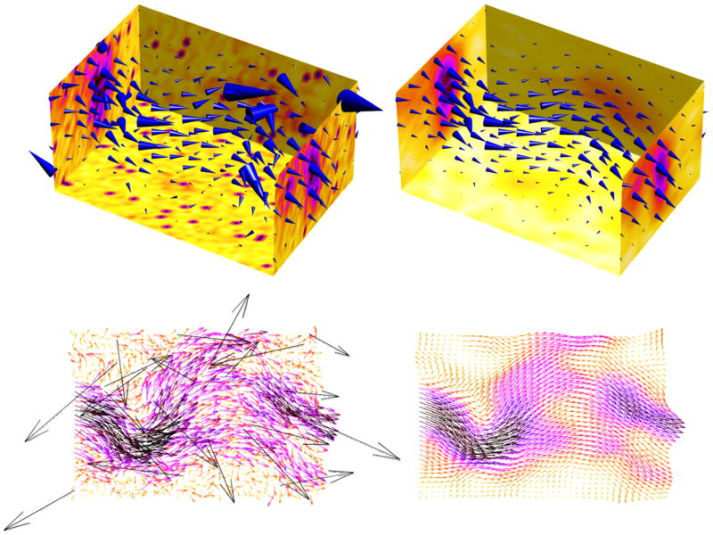
The DCT-based penalized least squares (DCT-PLS) method has been thoroughly described for evenly-spaced data in one and higher dimensions (Garcia 2010b). Because typical PIV data are equally gridded, the DCT-PLS can be efficiently applied to such data, as briefly introduced in the present section. For simplicity, only planar two-component velocity fields will be considered in this study although the method can be immediately applied to volumetric three-component velocity fields (see Figure 13 for one example).

Figure 13.

Automated post-processing of a 3-D corrupt mock flow (left versus right panels) with the DCT-PLS method. The bottom panels display the velocity field on a horizontal x-y plane at the middle of the volume of interest before (left) and after (right) post-processing.

Automatic smoothing with the DCT-PLS

Let us write the 2-D raw m×n velocity field V = (V_x, V_y), where V_x and V_y are the usual Cartesian velocity components. Assuming first that the PIV data are corrupted by experimental noise only (i.e. no outliers, no missing data), the DCT-PLS yields a smoothed velocity field V̂ from the following equation (Garcia 2010b):

$$\widehat{\mathit{V}}=\text{IDCT}2(\mathrm{\Gamma }\circ \text{DCT}2(\mathit{V})),$$ (2)

where DCT2 and IDCT2 refer to the type II 2-D discrete cosine transform and inverse discrete cosine transform, respectively, and ∘ stands for the Schur (elementwise) product. The filtering matrix Γ is defined by

$${\mathrm{\Gamma }}_{kl}={\left(1+s{\left(4-2cos\frac{(k-1)\pi }{m}-2cos\frac{(l-1)\pi }{n}\right)}^2\right)}^{-1}.$$ (3)

Equation (3) includes a real positive scalar s that controls the degree of smoothing: as the s parameter increases, the smoothing of V̂ also increases. An unsuitable selection for s could lead to under- or over-smoothed velocities. To avoid any subjectivity in the choice of the amount of smoothness, this parameter can be determined by minimizing the so-called generalized cross-validation (GCV) score (Craven et al. 1978). In the particular case of the DCT-PLS, the GCV score can be simplified as demonstrated in (Garcia 2010b). Minimization of the GCV score helps to optimize the trade-off between bias and variance: the bias measures how well the smoothed velocity field V̂ approximates the true velocity field V⁰, and the variance measures how well the original experimental data field V can be estimated by V̂. Excellent results are expected if the additive noise (ε) in Eq. (1) is Gaussian white (Wahba 1990). It has also been reported that the GCV remains fairly suitable even with nonhomogenous variances and non-Gaussian errors (Wahba 1990). The GCV criterion makes the DCT-PLS fully automated and is very well adapted to PIV data as shown further in the next sections.

Spatial frequency analysis of the DCT-PLS: effect of the smoothness parameter

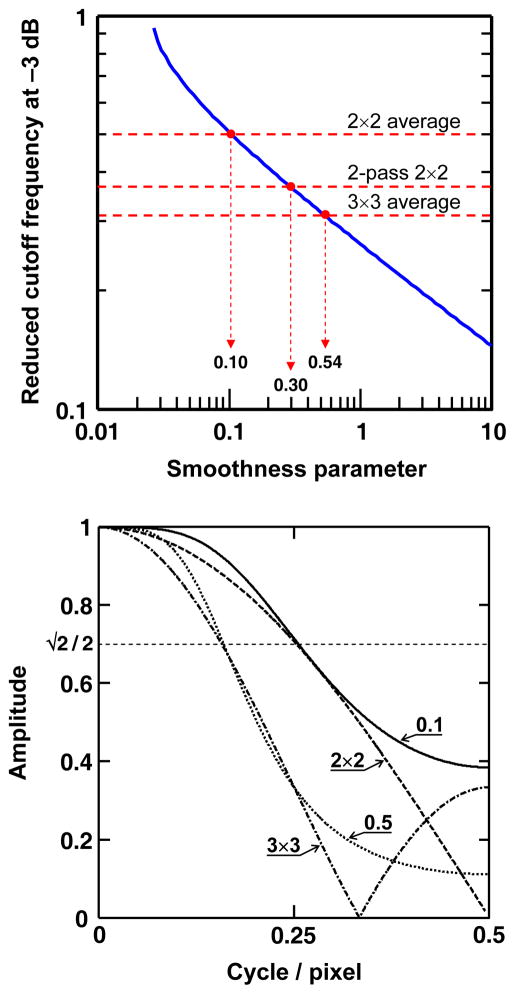
As stated in the latter paragraph, smoothness of the velocity field increases when s increases. When s runs from 0 to ∞, the output runs from the unchanged (original) data to the arithmetic mean of the velocities. In the spectral domain, increasing the smoothness parameter reduces the low-pass filter bandwidth. An exaggeratedly high s can lead to the loss of high spatial frequency components as may occur with turbulence or high shear flow. One thus has to ensure that the optimal s, i.e. the s value that minimizes the GCV score, prevents oversmoothing. Craven and Wahba have shown that the s value that minimizes the GCV score is also a fair minimizer of the mean square error (MSE) between the estimator and the actual value (Craven et al. 1978). In the context of PIV data, the optimal s thus provides the best guess V̂ of V⁰ (see equation 1) in the MSE sense. This assertion is essentially true with a Gaussian white noise process. To better appreciate how s influences the smoothing process, figure 1 (top panel) compares the s-dependent cut-off frequencies at −3dB of the DCT-PLS with those of small kernel average smoothers. As shown in this figure, the DCT-PLS has a cut-off frequency identical to that of 2×2, 2-pass 2×2 and 3×3 kernel average smoothers for s = 0.1, 0.3 and 0.5, respectively. Using a similar approach as in (Foucaut et al. 2002), the spatial frequency response (SFR) of the DCT-PLS was also determined for s = 0.1 and 0.5 and compared with the SFR of 2×2 and 3×3 moving average filters (Fig. 1, bottom panel). Ideally, s should be smaller than 0.5 in order the DCT-PLS to be compatible with the conventional smoothing methods. It is worth mentioning, however, that the optimal s highly depends upon the variance of the additive noise. Optimal values larger than 0.5 are thus expected with low-SNR (signal-to-noise ratio) PIV data. In that case, the smoothness parameter can be set manually at a low level, say smaller than 0.5; one must be aware, however, that this can lead to undersmoothing if the PIV data have a low SNR.

Figure 1.

Top panel: Reduced cut-off frequency of the DCT-PLS (at −3dB) as a function of the smoothness parameter (s). The cut-off frequencies of common average filters are also represented (dashed horizontal lines). Bottom panel: Spatial frequency responses (SFR) of the DCT-PLS for two s values (0.1 and 0.5). The SFR of the 2×2 and 3×3 average filters are depicted for comparison. The dashed horizontal line corresponds to the −3dB limit.

Replacement of the outlying data with the DCT-PLS

Besides experimental noise, PIV data typically contain spurious vectors mostly due to the loss of correlation signal in case of insufficient particle seeding, out-of-plane motions or strong gradients. If neglected, the outlying vectors may make the smoothed PIV field abnormally distorted. To overcome this drawback, the DCT-PLS uses a robust procedure that is very little affected by the outliers. This method consists in constructing weights with a specified weighting function by using the current residuals and updating them, from iteration to iteration, until the residuals remain unchanged. It is worth noting that the DCT-PLS does not contain any “outlier detector” based on a specific predicate such as used in the normalized median test. The algorithm rather assigns a low weight to outlying values in order to reduce their influence. The robust version of DCT-PLS is given by the following implicit formula (see (Garcia 2010b) for more details):

$$\widehat{\mathit{V}}=\text{IDCT}2\left(\mathrm{\Gamma }\circ \text{DCT}2\left(W^{bs}\circ (\mathit{V}-\widehat{\mathit{V}})+\widehat{\mathit{V}}\right)\right),$$ (4)

This equation can be solved using a fixed point iteration with V̂ = V as initial conditions. The matrix W^bs contains the bisquare weights which depend upon the so-called studentized residuals (Heiberger et al. 1992). In the case of the DCT-PLS, the studentized residuals can be extremely simplified to make the algorithm faster (Garcia 2010b).

Dealing with missing values and masks

Missing values can also occur due to masking materials, laser reverberations or defects in the CCD camera sensor. In addition, the region of interest (ROI) and the area enclosed by the PIV raw images do not always coincide. Missing vectors and areas to be masked thus need to be extracted before any postprocessing. The DCT-PLS can easily cope with missing and masked data by introducing a second weight matrix, W^m, defined by $W_{kl}^m=0$ if the velocity in pixel (k,l) is masked or missing, 1 otherwise. Equation (4) thus becomes:

$$\widehat{\mathit{V}}=\text{IDCT}2\left(\mathrm{\Gamma }\circ \text{DCT}2\left(W^m\circ W^{bs}\circ (\mathit{V}-\widehat{\mathit{V}})+\widehat{\mathit{V}}\right)\right).$$ (5)

Equation (5) is the generalized equation of the robust DCT-PLS applied to PIV velocity data.

Matlab code

The use of equation (5) provides a post-processed velocity field by removing noise, missing data and outliers conjointly and automatically. Further details regarding the smoothing algorithm can be found in (Garcia 2010b). Because the procedure mostly involves DCTs, the numerical scheme can be made very fast. A Matlab code written with Matlab R2008b is given in the supplemental material (see appendix). Updated versions can be downloaded from the author’s personal website (Garcia 2010a). The efficacy of the DCT-PLS is demonstrated in the following sections by post-processing simulated and experimental PIV fields. Several results obtained with the DCT-PLS are compared with those issued from the conventional post-processing methods.

3. Processing of outlying and noisy velocities: conventional methods vs. DCT-PLS

Following Shinneeb et al (Shinneeb et al. 2004), and in order to quantify the accuracy of the proposed method, the DCT-PLS was tested on simulated vortical cellular flows with additional noise and outliers. The original m×n velocity field (V⁰), containing four vortical cells, was defined by the following Cartesian components:

$${\mathit{V}}_{kl}^0=V_{max}\left\{sin\left(2\pi \frac{k-1}{m-1}\right)cos\left(2\pi \frac{l-1}{n-1}\right);-cos\left(2\pi \frac{k-1}{m-1}\right)sin\left(2\pi \frac{l-1}{n-1}\right)\right\},$$ (6)

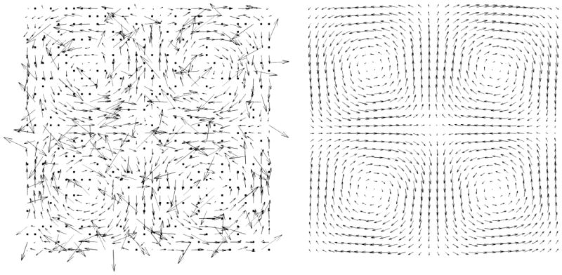
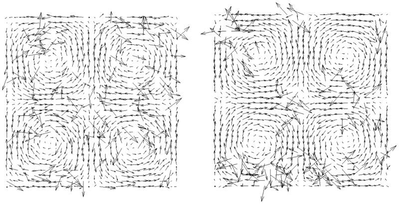
where V_max stands for the maximal velocity. Figure 2 illustrates such a vortical flow in the particular case of (m,n) = (32,32) which has been made exaggeratedly corrupt by the addition of random noise, spurious vectors and missing data (Figure 2, left). Despite high deterioration of the velocity data, the DCT-PLS is clearly able to recover the imprint of the actual flow field (Figure 2, right). To better represent real PIV measurements, numerical tests were performed on 32×32 fields with random noise and spurious vectors as defined below. A value of 10 pixels/pulse-interval was chosen for the maximal velocity V_max. Gaussian noise with mean zero and constant variance was first included on both x- and y-components of the original velocity field. Two variances were tested, (0.01×V_max)² and (0.1×V_max)². Spurious (outlying) velocity vectors were then added using either scattered or clustered patterns (Shinneeb et al. 2004). Spurious data were defined as vectors whose x-and y-components were drawn independently from a uniform distribution on the interval [−2V_max ; 2V_max]. By way of example, two noisy synthetic PIV fields with 15% of spurious vectors in both scattered and clustered configurations are illustrated in Figure 3. In the scattered configuration (Figure 3, left), the spurious velocities were randomly and uniformly distributed throughout the whole field. In practice, however, spurious vectors often appear at the edges of the PIV field, near model surfaces, on low seeded areas, and on regions poorly or highly illuminated. Under these conditions, spurious vectors are found in clusters. In the simulated clustered organizations (Figure 3, right), the groups were positioned randomly and their sizes were chosen from a Poisson distribution with mean six. Four scenarios were thus analyzed: 2 Gaussian noises × 2 spurious arrangements. For each scenario, the relative amount of spurious vectors was ranged from 0 to 25% with an increment of 2.5% which represented a total of 4×11 = 44 cases. Finally, 100 PIV fields were created based on a Monte-Carlo method for each of these cases. The simulated PIV data were analyzed using both a conventional post-processing and the DCT-PLS described in this paper. The conventional method consisted in 1) validating the data by means of the normalized median test using 2.0 for the threshold and 0.1 for the noise level, as recommended (Raffel et al. 2007; Westerweel et al. 2005), 2), replacing the invalid vectors by the median of the 3×3 neighborhood and, 3) smoothing the entire field using a 3×3 averaging kernel. These successive conventional processes were performed with the free package for particle image velocimetry, JPIV, written by P. Vennemann (Vennemann 2008; Vennemann 2009). The simulated PIV fields were also post-processed by means of the new DCT-PLS technique which was made fully automated using the abovementioned GCV score. The DCT-PLS was entirely programmed in Matlab language (The MathWorks, Natick, MA, USA; see also appendix). The performances of the two methods were compared by using the normalized root mean squared error (NRMSE) between the original (V⁰) and the post-processed (V̂) velocity fields given by:

$$\mathit{NRMSE}=\frac{{\Vert \widehat{\mathit{V}}-{\mathit{V}}^0\Vert }_F}{{\Vert {\mathit{V}}^0\Vert }_F}\times 100,$$ (7)

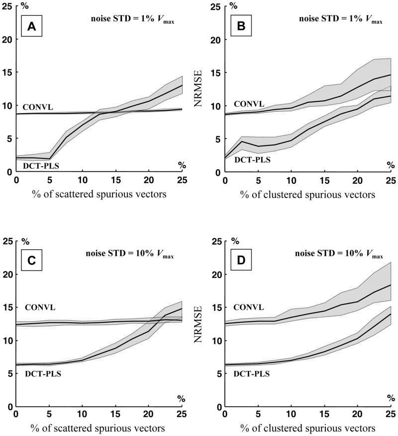
where || ||_F denotes the Frobenius norm. The median, lower and upper quartiles of the NRMSE were plotted as a function of the percentage of spurious vectors for each of the four scenarios (Figure 4).

Figure 2.

Vortical cellular flow (32×32) corrupted by Gaussian noise, outliers and missing data before (left) and after (right) smoothing by the DCT-PLS. The normalized root mean squared error (NRMSE, see equation 7) was 14% here.

Figure 3.

Vortical cellular flow (32×32) corrupted by a Gaussian noise of variance (0.01×V_max)² and 15% of outlying vectors. Two configurations were tested in this study: scattered (left) and clustered (right) spurious vectors.

Figure 4.

Normalized root mean squared errors (NRMSE, see equation 7) between the original and the post-processed vortical flow fields, as a function of the percentage of outlying vectors, in the following situations: A and B: Gaussian noise with standard deviation (STD) 1% V_max, with scattered (A) and clustered (B) spurious vectors; C and D: Gaussian noise with standard deviation 10% V_max, with scattered (C) and clustered (D) spurious vectors. CONVL stands for the conventional method while DCT-PLS represents the DCT-based penalized least squares method.

Figures 4A and 4C show that the conventional method resulted in ~8% and ~12% errors with the scattered patterns and noise variances of (0.01×V_max)² and (0.1×V_max)², respectively. In the scattered configuration, the errors related to the conventional method (CONVL) were independent of the number of spurious vectors. This means that the normalized median test (Westerweel et al. 2005) was highly efficient in detecting the scattered spurious vectors, even in large number. The remaining errors were thus mostly due to the noise which was not completely removed by the smoothing kernels. Because the normalized median test identifies the outliers by comparing the vectors with their neighbors, it lost some effectiveness with the clustered arrangements beyond 10% of outliers (Figures 4B and 4D). The normalized errors with the DCT-PLS method increased when increasing the percentage of spurious vectors. The DCT-PLS provided better results than the conventional method with the clustered outlying vectors (Figures 4B and 4D). With scattered outliers and low-variance noise, the conventional method yielded lower errors beyond 15% of spurious data (Figure 4A). High-quality PIV fields, however, typically contain no more than 10% of spurious velocities, in which case the DCT-PLS provides improved post-processed velocity fields in comparison with the conventional method (<7% vs. <13% see Figures 4A-D). It is worth noting that the DCT-PLS method does not consider only the neighborhood of the data to be replaced but actually takes the entire field into account. This makes the DCT-PLS little dependent upon the outliers’ distribution.

4. The DCT-PLS with missing values and masks

Dealing with occurrence of missing data

Dropouts or missing data can sometimes occur in PIV measurements due to experimental hazards or minor material defects. How the DCT-PLS can deal with missing values was analyzed on the 32×32 vortical flow (equation 6) with additive Gaussian noise of variance (0.1×V_max)². An amount of 0 to 50% (using an increment of 5%) of clustered missing data was included within the original PIV field using random Poisson distributions with mean six, as described in the previous section. One hundred Monte-Carlo simulations per configuration were performed. The median, lower and upper quartiles of the corresponding NRMSE (see equation 7) are given in Figure 5. The NRMSE remained relatively low (<8%) even with 50% of missing vectors and was mostly influenced by the additive noise. These results confirm that the DCT-PLS is highly robust to missing data.

Figure 5.

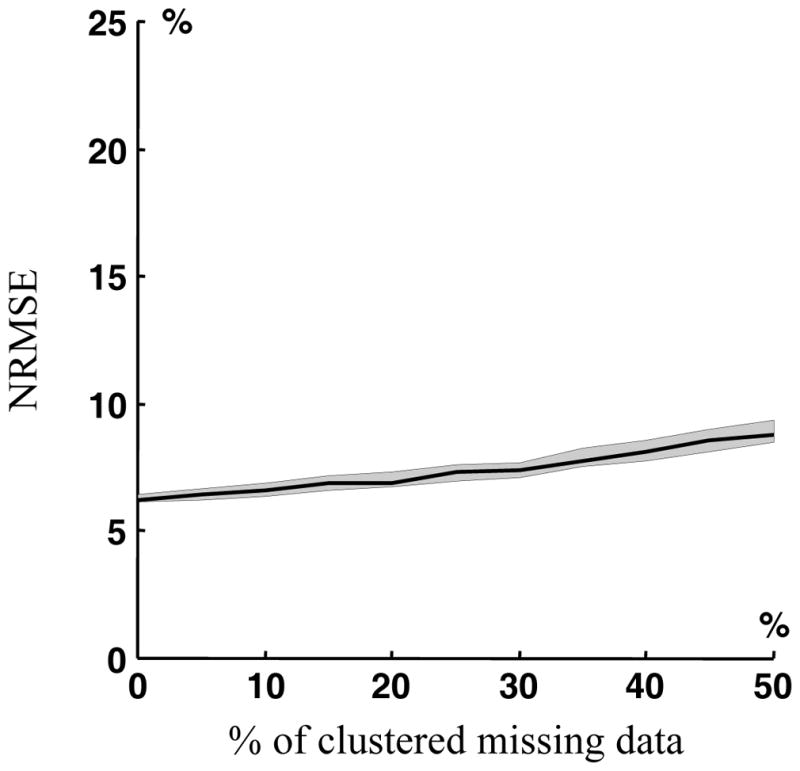
Effect of clustered missing data on the post-process of the vortical flow (noise STD = 10% V_max) with the DCT-PLS: normalized root mean squared errors (between the post-processed and original velocity fields) as a function of percentage of missing vectors.

Application of the DCT-PLS with masks

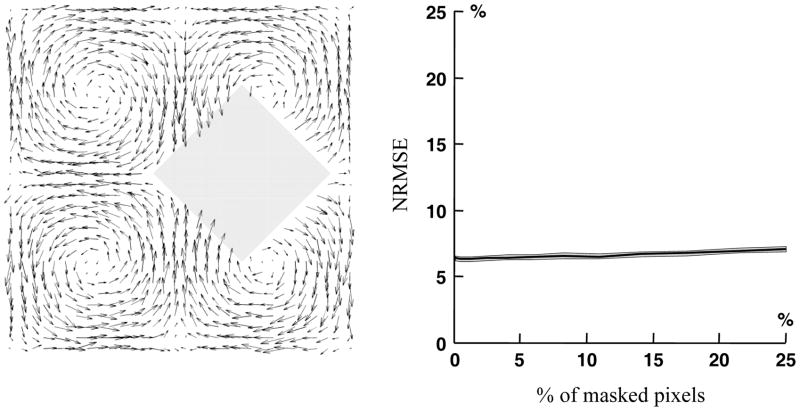
The fast DCT and inverse DCT transforms only work with data gridded evenly on rectangles (or N-orthotopes in N dimensions). In the case of a masked PIV field, the region of interest becomes non rectangular (or non orthotopic). However, as described by equation (5), masking can be taken into account by associating nil weights to masked pixels so that they do not influence the DCT-PLS process. To illustrate that the DCT-PLS can readily deal with masks, several series of Monte-Carlo simulations were completed as described in the previous paragraph. Instead of including missing values, however, randomly positioned diamond-shaped masks of varying radii (from 0 to 11 pixels) were added. Figure 6A illustrates such a PIV field with a diamond-shaped mask of radius 8. The NRMSE obtained with masked PIV fields (figure 6B) shows that the masks have very little effect on the smoothing process.

Figure 6.

Effect of masks on the post-process of the vortical flow (noise STD = 10% V_max) with the DCT-PLS. Left panel: one example with a diamond-shaped mask of radius 8 pixels. Right panel: normalized root mean squared errors (between the post-processed and original velocity fields) as a function of percentage of masked pixels.

5. The DCT-PLS method with experimental PIV data

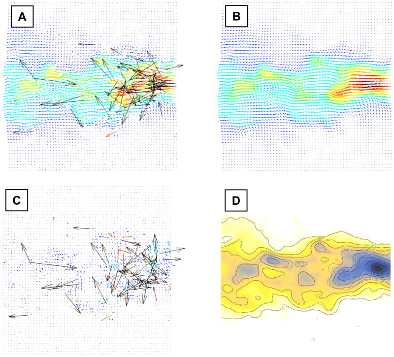
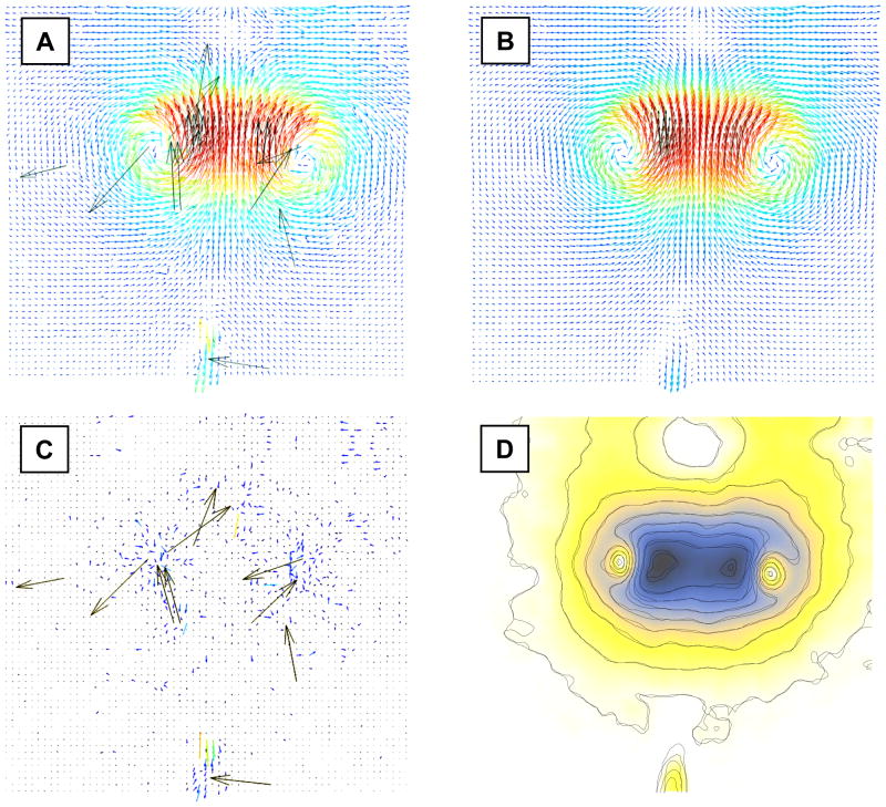
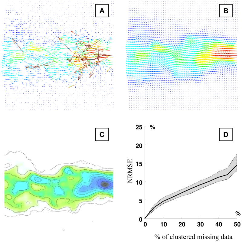
To verify that the new method proposed in this paper is also suitable to real PIV data, the DCT-PLS was tested on two experimental PIV image series freely accessible online. The first image pair, provided by J. Westerweel (Westerweel et al. 2005), represents a free turbulent jet and is available from PIV challenge (Okamoto 2003). The second image series was acquired in a vortex pair (Willert et al. 1997) and is downloadable from the PIVTEC website (PIVTEC 2009). The image pairs were evaluated by PIVview2C Demo (version 2.4, PIVTEC GmbH, Göttingen, Germany) with a 32×32 (turbulent jet, Figure 7A) or 16×16 (vortex pair, Figure 8A) interrogation window using a standard single-pass cross-correlation and a 50% window overlap. The raw pixel shift data were saved in ASCII files and post-processed with the DCT-PLS. As illustrated by Figures 7A and 8A, the raw PIV fields contained spurious vectors that were all eliminated by the DCT-PLS (Figures 7B and 8B). A closer look at the residuals (Figures 7C and 8C) reveals that the DCT-PLS method also removed spurious velocity components of small magnitude. It is worth noticing (Figures 7D and 8D) that significant differences appeared between the smoothed fields returned by the DCT-PLS and the conventional method (normalized median filter + 3×3 average kernel). This difference is particularly notable in the jet inflow (Figure 7D), which is likely due to the presence of numerous outliers (see Figure 7A). The overall normalized differences between the two methods (defined as: 2||V_DCT-PLS – V_CONVL||_F / [||V_DCT-PLS||_F + ||V_CONVL||_F]) were 7.6% and 3.6% for the jet and vortex patterns, respectively.

Figure 7.

Experimental PIV data measured in a turbulent jet (from Westerweel et al., see text for details). A) Raw PIV velocities. B) PIV velocities post-processed with the DCT-PLS. C) Residuals (velocities in A – velocities in B). D) Contour plots of the velocity magnitudes (solid lines: using the DCT-PLS, dashed lines: using the conventional method). The background represents the velocity magnitudes obtained with the DCT-PLS (Fig. 7B).

Figure 8.

Experimental PIV data of a vortex pair (from Willert et al., see text for details). A) Raw PIV velocities. B) PIV velocities post-processed with the DCT-PLS. C) Residuals (velocities in A – velocities in B). D) Contour plots of the velocity magnitudes (solid lines: using the DCT-PLS, dashed lines: using the conventional method). The background represents the velocity magnitudes obtained with the DCT-PLS (Fig. 8B).

Missing data

As in section 4, an amount of 5 to 50% (with an increment of 5%) of clustered missing data was included within the original PIV data of the turbulent free jet using random Poisson distributions with mean six. Again, 100 Monte-Carlo simulations per arrangement were carried out. The post-processed PIV fields (V̂) with missing vectors were compared to the post-processed PIV field without missing data (V̂_0%) by means of the following NRMSE:

$$\mathit{NRMSE}=\frac{{\Vert \widehat{\mathit{V}}-{\widehat{\mathit{V}}}_{0\%}\Vert }_F}{{\Vert {\widehat{\mathit{V}}}_{0\%}\Vert }_F}\times 100.$$ (8)

The median, lower and upper quartiles of the NRMSE were plotted as a function of the percentage of missing data. An example with 50% of missing values is given by Figure 9A (see also Figure 7A for comparison). Although this case represents an unrealistic PIV pattern, it clearly illustrates that the DCT-PLS can efficiently cope with missing vectors. In spite of high degradation, the velocity field was indeed reconstructed with reasonable accuracy (Figures 9B–C). As expected, the normalized error increased when increasing the number of missing vectors but remained less than 10% with an amount of missing velocities as large as 30% (Figure 9D).

Figure 9.

Efficiency of the DCT-PLS with missing data. A) 50% of vectors have been randomly removed from the raw PIV velocities illustrated in Fig. 7A. B) The DCT-PLS reconstructed the velocity field with reasonable accuracy (compare with Fig. 7B). C) Contour plots of the velocity magnitudes (solid lines: using the DCT-PLS on the raw PIV data of Fig. 7A, dashed lines: using the DCT-PLS on the modified raw PIV data of Fig. 9A). The background represents the velocity magnitude obtained with the original raw data (Fig. 7B). D) Effect of the percentage of missing vectors on the normalized root mean squared error (NRMSE, see equation 8) between the post-processed PIV fields with missing vectors (turbulent jet, see Fig. 9B) and the post-processed PIV field without missing data (see Fig. 7B).

Masked region-of-interest

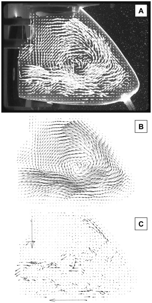
The DCT-PLS was finally used to post-process PIV raw velocities measured in an in vitro left ventricle, supplied by the cardiovascular biomechanics team of the IRPHE (Institut de recherche sur les phénomènes hors équilibre, Marseilles, France) (Garcia et al. 2010; Tanné et al. 2010). These PIV data decipher the intraventricular velocity field during early diastole (ventricular relaxation). As depicted in Figure10A, we were interested in the flow delimited by the left ventricular wall. The blood-mimicking fluid enters the left ventricle through the mitral valve and forms a large vortex that remains until the onset of left ventricular contraction. Figures 10B and 10C represent the smoothed velocity field resulting from the DCT-PLS and the residuals, respectively. These results demonstrate that the DCT-PLS worked rightly within the non rectangular cardiac cavity.

Figure 10.

Application of the DCT-PLS approach with PIV measurements performed in a left ventricular model (IRPHE, Marseilles, France). From top to bottom: A) raw PIV data, B) PIV velocity field post-processed with the DCT-PLS, C) residuals.

6. Limitation of the DCT-PLS and application to 3-D data

The DCT-PLS with high velocity gradients

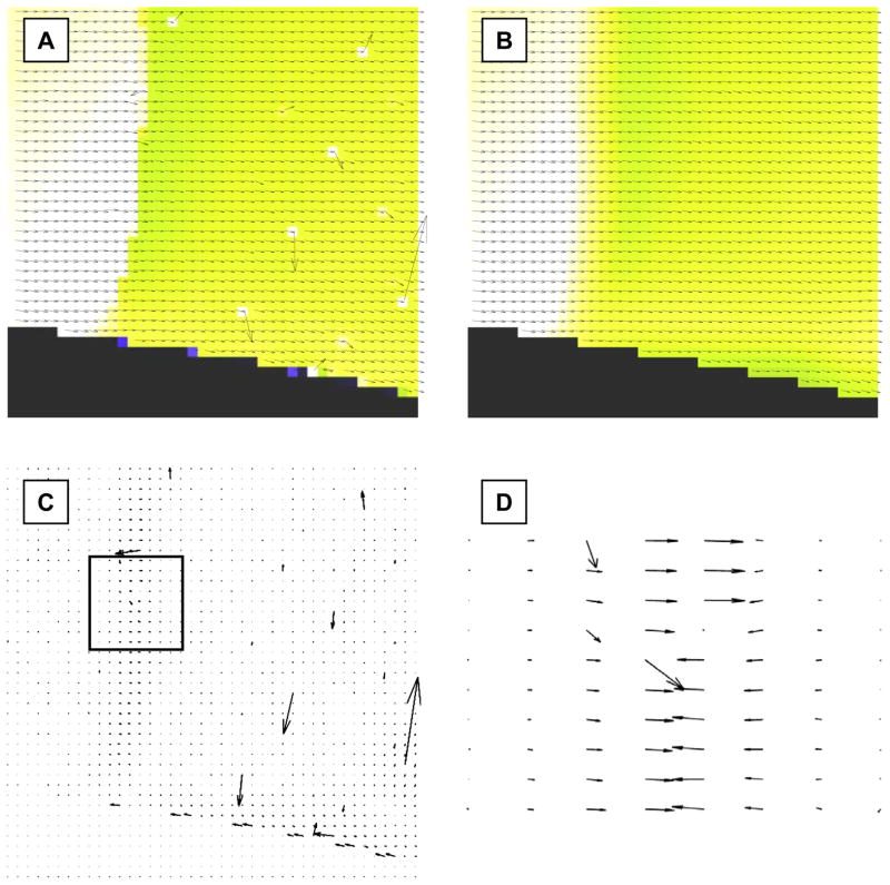
The examples provided in the present manuscript show that the DCT-PLS can post-process PIV fields very efficiently in numerous instances. One noteworthy limitation of the algorithm, however, should be addressed: better results will be obtained if the velocity field to be sought (V⁰, see equation 1) is sufficiently smooth (i.e. if it contains continuous derivatives in both directions up to some order over the whole domain of interest). This may not be the case in the presence of supersonic flows where velocity discontinuities may occur. In such situation, the DCT-PLS can tend to over-smooth the velocity step gradients that appear along the shock waves. As depicted in Fig 1 and discussed above, the DCT-PLS behaves similarly to a 2×2 or 3×3 moving average (in terms of cut-off frequency) when s is in the range [0.1–0.5]. As a consequence, the original PIV field must preferably not be too noisy so that the optimal smoothness parameter remains lower than 0.5. The optimal s (issued from the GCV score minimization) calculated with the three experimental data (Figures 7, 8 and 10) were all less than 0.5 (0.18, 0.38 and 0.21). Although this remains to be confirmed with more velocity fields, the results reported in this study tend to show that the optimal s values are in the range [0.1–0.5] for experimental subsonic PIV data, which ensures that oversmoothing should be avoided in most cases. Alternatively, the DCT-PLS can be used with a very low smoothness parameter (without GCV score minimization) to reduce the effect of smoothing. Nonetheless, even with a low s value, the DCT-PLS may oversmooth high step gradients. As an example, Figure 11A depicts a transonic flow containing velocity discontinuities (courtesy of Dr. Kompenhans and Dr. Schroeder from DLR’s institute of aerodynamics and flow technology, Göttingen, Germany), and illustrates the effect of the DCT-PLS on such PIV data (Fig. 11B). Oversmoothing clearly appears along the shock wave (Figures 11C-D), which may limit the use of the DCT-PLS in the presence of supersonic flows.

Figure 11.

Oversmoothing due to the DCT-PLS with a supersonic flow (courtesy of Dr. Kompenhans and Dr. Schroeder, DLR’s institute of aerodynamics and flow technology). A) Raw PIV data. B) PIV velocity field post-processed with the DCT-PLS. C) Difference between the raw and post-processed fields. D) Close-up that reveals the presence of oversmoothing along the shock wave.

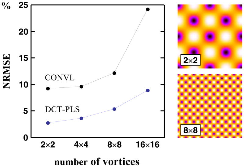
Besides the presence of high step gradients, the DCT-PLS can also be limited if the region of interest is not adequately sampled (i.e. is characterized by a low spatial resolution). As shown in Figure 12, the NRMSE indeed increases as the number of vortices augments for a given resolution (field size = 128×128, noise variance = (0.1×V_max)², 10% of scattered spurious vectors). This result is not surprising since this would occur with any nonparametric smoother, like the 3×3 moving average filter. It must be noticed, however, that the DCT-PLS still provides better outputs than the conventional method (see Fig. 12).

Figure 12.

Left panel: effect of the number of vortices on the normalized root mean squared error (NRMSE): comparison between the DCT-PLS and the conventional method (CONVL). Velocity field size = 128×128, noise standard deviation = 0.1×V_max, percentage of spurious vectors = 10%. Right panels: two velocity amplitude fields (before being corrupted) are represented for an illustrative purpose (2×2 and 8×8 vortices).

Application to volumetric PIV data

Volumetric three-component PIV is now available (Elsinga et al. 2006; Pereira et al. 2006) and can provide a complete three-dimensional velocity field in a rectangular parallelepiped. Although this paper is focused on two-dimensional velocity fields exclusively, the algorithm is immediately applicable to three and higher dimensions (Garcia 2010b). To test its suitability to post-process three-dimensional (3-D) velocity field, the DCT-PLS was finally used on a 3-D mock flow altered by noise, missing data and outliers. This synthetic flow, of size 35×41×15, was created using the “wind” data available in Matlab (Fig 13). Several Monte-Carlo simulations were also performed to quantify the effect of scattered spurious vectors (methodology similar to section 3). As shown on Figures 13 and 14, the new postprocessing method can efficiently smooth 3-D velocity fields as well.

Figure 14.

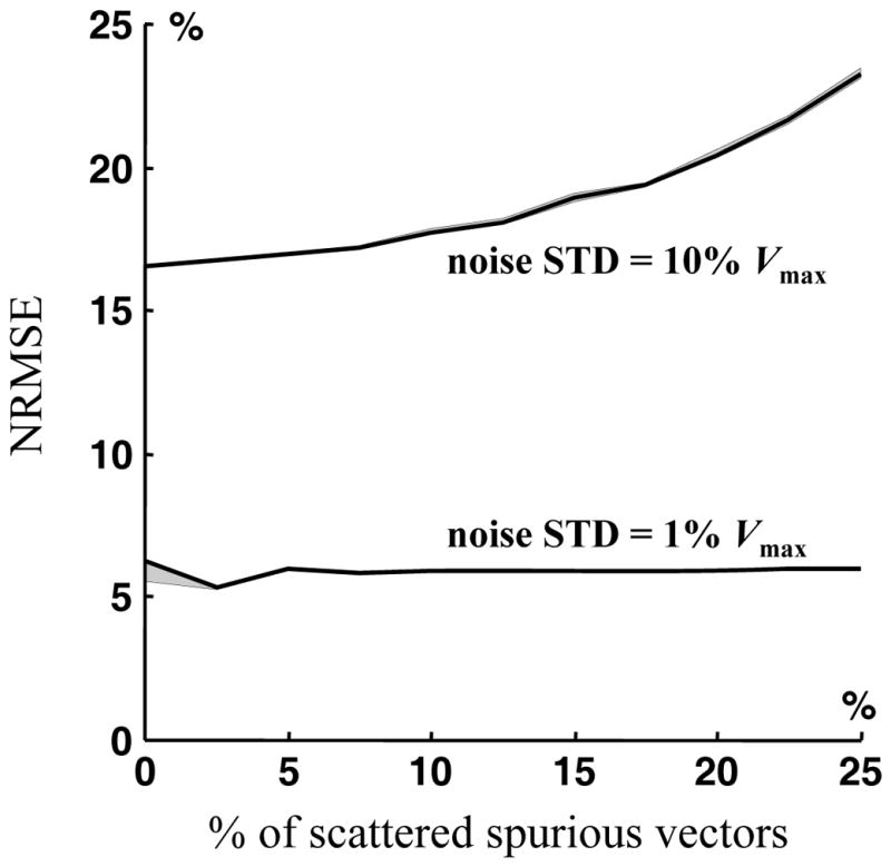
Normalized root mean squared errors between the post-processed and original velocity fields (NRMSE, see equation 7) as a function of percentage of spurious vectors in the 3-D mock flow (see also Fig 13). Two noise standard variations were tested: 0.1 V_max and 0.01 V_max.

7. Conclusion

Conventional post-processing of PIV velocity fields typically requires three consecutive steps, namely, validation, replacement of the incorrect data, and smoothing. The DCT-based penalized least squares (DCT-PLS) method described in this paper can handle experimental noise, outliers and missing data, simultaneously. As demonstrated by our results, the DCT-PLS is very well adapted to raw PIV data due to its efficiency, accuracy and rapidness. In addition, contrary to other methods, the DCT-PLS is an automatic all-in-one process and does not require any subjective adjustment of thresholding parameters or kernel sizes. More importantly, the DCT-PLS is independent of the outliers’ distribution while the conventional median test is less efficient when the spurious vectors are clustered, as often occurs in practice. Because it makes use of the fast discrete cosine transform, the DCT-PLS is as computationally fast as the conventional methods and much faster than alternative methods recently published.

Appendix

The supplemental material contains one Matlab program (pppiv, Post-Processing of PIV data) that includes all the properties described in this paper. It carries out automatic and robust post-processing of 2-D PIV data. Enter “help pppiv” in the Matlab command window to obtain a detailed description, the syntax for pppiv and one example. Updated versions of pppiv are also downloadable from the author’s personal website (Garcia 2010a).