FRACTIONAL INTEGRATION TOOLBOX

Abstract

The problems formulated in the fractional calculus framework often require numerical fractional integration/differentiation of large data sets. Several existing fractional control toolboxes are capable of performing fractional calculus operations, however, none of them can efficiently perform numerical integration on multiple large data sequences. We developed a Fractional Integration Toolbox (FIT), which efficiently performs fractional numerical integration/differentiation of the Riemann-Liouville type on large data sequences. The toolbox allows parallelization and is designed to be deployed on both CPU and GPU platforms.

1. Introduction

In the last several decades many processes in biology, pharmacology, chemistry, physics, engineering and finances have been formulated in the firamework of fractional calculus [1], [2], [7], [8], [18]-[20].

Systems involving fractional processes exhibit residual memory and their fractional order is interpreted ([12], [13], [15]) as a measure of the memory strength, which depending on the fractional order α, positions them somewhere between complete memory and Markovian systems [13].

For practical applications such as fractional diffusion-reaction or other fractional dynamical systems simulations, it is sometimes necessary to calculate the fractional Riemann-Liouville (RL) integral of a function f(τ), given by:

$${\mathrm{I}}_t^{\alpha }f\left(t\right)=\frac{1}{\Gamma \left(\alpha \right)}{\int }_0^t{(t-\tau )}^{\alpha -1}f\left(\tau \right)d\tau$$ (1.1)

where Γ(α) is Euler’s gamma function and α is positive real number.

For each spatial point x_i at each time step τ_j of the simulation, one needs to estimate numerically eq.(1.1) given the sequence f (τ₁), f (τ₂),…, f (τ_j) obtained from the previous steps of the simulation. Even for a relatively large spatial discretization step in a one dimensional fractional diffusion-reaction simulation, the numerical evaluation of eq.(1.1) becomes computationally prohibitive in terms of speed and memory requirements due to the increasing size of the input matrix. This problem becomes even more severe in the case of a simulation of multiple fractional diffusion-reaction equations describing the interactions in a biochemical reaction or in the case of multidimensional simulations. Furthermore, achieving higher accuracy of the numerical quadrature of eq.(1.1) involves multistep methods, which require even more computational resources.

While there are several fractional control toolboxes (Crone [11], Fomcon [22], Ninteger [23]) capable of performing fractional calculus operations, none of them is designed to fractionally integrate simultaneously multiple sequences of large length.

Here we report the development of a Fractional Integration Toolbox (available for download at www.cbi.utsa.edu/projects/faculty) which employs an efficient algorithm [5] and allows the user to choose computational platforms (CPU, GPU) and parallelization (openMP). Our Benchmark test shows that integration in High Performance platforms can achieve speed improvement of two orders of magnitude. This enables applications which require simultaneous fractional integration of multiple data sources in real time. For completeness we have included an efficient numerical routine [14] for fractional derivatives of the RL type.

The toolbox is generic. It can be used both in a standalone and in a simulation mode. The standalone mode fractionally integrates an arbitrary set of data. The simulation mode is designed for the case when repeated fractional integration is performed on sets of data, which increase one term at a time. In that case additional performance optimization is possible. This makes FIT a beneficial tool not only in the case of fractional reaction-diffusion studies, but also to other fields formulated in terms of fractional dynamics.

2. Methods

For the fractional integration we consider only fractional integrals of the RL type and employ the numerical algorithm provided in [5]. This algorithm is valid for any α > 0. On the interval [0,T] with equally spaced points t_n = nh : n = 0, 1…, N , where h = T/N , the integral’s (eq.(1.1)) leading order approximation is given by

$$\begin{array}{cc}\hfill I^{\alpha }fN\left(h\right)& =\frac{h^{\alpha }}{\Gamma (2+\alpha )}\sum _{n=0}^N{c}_n,Nfn\hfill \\ \hfill I^{\alpha }f\left(T\right)& =I^{\alpha }fN\left(h\right)+O\left(h^2\right)\hfill \end{array}$$ (2.1)

where f_n = f (t_n) and c_n,N are the quadrature weight coefficients

$$c_n,N=\{\begin{array}{cc}(1+\alpha )N^{\alpha }-N^{1+\alpha }+{(N-1)}^{1+\alpha }\hfill & n=0;\hfill \\ {(N-n+1)}^{1+\alpha }-2{(N-n)}^{1+\alpha }+{(N-n-1)}^{1+\alpha }\hfill & 1<n<N;\hfill \\ 1\hfill & n=N;\hfill \end{array}\phantom{\}}$$ (2.2)

derived from a product trapezoidal rule.

Further refinement is possible by using the Richardson extrapolation:

$$\begin{array}{cc}\hfill I^{\alpha }{f}_v^u\left(T\right)& =(I^{\alpha }{f}_{v-1}^{u-1}\left(T\right)-2^{r_{u-1}}{I}^{\alpha }{f}_v^{v-1}\left(T\right))∕(1-2^{r_{u-1}}),\hfill \\ \hfill I^{\alpha }f\left(T\right)& =I^a{f}_v^u\left(T\right)+O\left(h^{r_u}\right),\hfill \end{array}$$ (2.3)

where

$$\begin{array}{cc}\hfill & I^{\alpha }{f}_0^0\left(T\right)=I^{\alpha }fN\left(h\right)\hfill \\ \hfill & I^{\alpha }{f}_1^0\left(T\right)=I^{\alpha }fN\left(\frac{h}{2}\right)\hfill \\ \hfill & .\hfill \\ \hfill & .\hfill \\ \hfill & .\hfill \end{array}$$ (2.4)

and the exponents r₀, r₁, r₂, … have to be ordered in a monotonic sequence, i.e.

$$\begin{array}{cc}\hfill & r_0=2,r_1=2+\alpha ,r_2=3,r_3=3+\alpha ,\dots \mathrm{for}0<\alpha <1,\hfill \\ \hfill & r_0=2,r_1=3,r_2=2+\alpha ,r_3=4,\dots \mathrm{for}1<\alpha <2,\hfill \\ \hfill & .\hfill \\ \hfill & .\hfill \\ \hfill & .\hfill \end{array}$$ (2.5)

Thus for a leading order and a first correction approximation:

$$\begin{array}{cc}\hfill I^{\alpha }{f}_1^1\left(T\right)& =\frac{I^{\alpha }{f}_0^0\left(T\right)-2^2{I}^{\alpha }{f}_1^0\left(T\right)}{1-2^2},\hfill \\ \hfill I^{\alpha }f\left(T\right)& =I^{\alpha }{f}_1^1\left(T\right)+O\left(h^{r_1}\right).\hfill \end{array}$$ (2.6)

The discretization of the function f (τ) depends on the chosen time step h. However, the calculation of the first correction requires the evaluation of f (τ) at the midpoints of each interval, i.e. at a time step h/2. Since the leading order is the exact solution of eq.(1.1), provided that f (τ ) is linearly interpolated in each of the intervals, there will be no gain in accuracy that could come from the calculation of the first correction based on resampled data from piecewise linear interpolation. In order to increase accuracy we use spline interpolation.

The FIT allows the user to choose between two types of spline interpolation, i.e. regular cubic splines and piecewise cubic Hermite interpolation. Cubic splines interpolate smooth functions very well due to the fact that they are constructed by piecewise smooth functions, matched at the nodes to preserve smoothness (matching both first and second derivatives). The piecewise cubic Hermite interpolation, on the other hand, is well suited to handle noisy data. It has minimal overshoots and undershoots and in general it follows better the behavior of piecewise continuous functions.

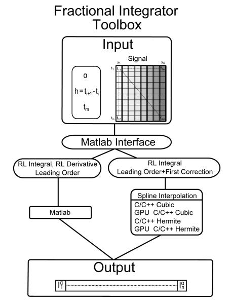
The data flow of the FIT is shown on Figure 1. The input for the toolbox includes the fractional order α, the discretization time step h, the integration limit t_m, as well as a m × n data matrix. Each of the columns of the data matrix represents a sequence of discrete values of the integrand f ( f_1i, f_2i,…,f_mi), which is to be numerically integrated/differentiated. As a result, the toolbox returns n integral/derivative values-one for each sequence of data points.

Figure 1.

Block diagram of the Fractional Integral Toolbox

The properties of the function to be integrated, such as size, stiffness or noise require the use of different integration algorithms. In order to provide a generic toolbox we have implemented multiple algorithms that can be chosen at the time of setup:

• Linear− leading order (LO)

• Cubic spline− leading order+correction

• Hermite spline− leading order+ correction

All of the integration algorithms are based on [5], however their implementations vary. The leading order approximation (eq.(2.1)) does not require interpolation and is implemented efficiently in MATLAB (Natick, MA) as a dot product of the vector containing the integration weights (eq.(2.2)) and the input matrix containing all the time signals. Since MATLAB supports implicit multithreading, the computation takes advantage of multicore computer architectures automatically. Additional acceleration is achieved through the use of highly efficient MATLAB vectorized notation.

The leading order+first correction approximation (eq.(2.6)) requires sampling at a time step h/2, i.e. interpolation is necessary. The FIT provides two separate interpolation methods- a regular cubic spline as well as Hermite piecewise cubic interpolation. For the setup of the cubic spline coefficients and the numerical solution of the resulting tridiagonal system we employ [3], [4], [21].

In the case of the Hermite piecewise cubic interpolation we obtain monotonic cubic polynomials by employing the algorithm described in [10]. Both the regular cubic and the Hermite piecewise cubic interpolation algorithms are implemented in C++ and are integrated with MATLAB via a MEX interface with OpenMP multithreading. For better performance the interpolated data needed for the calculation of the correction is not stored, but is generated and used dynamically. Additional simplification and improvement of efficiency is possible by taking advantage of the fixed time step in the spline midpoint evaluation. The FIT provides two more fractional integration options- a hybrid GPU+CPU Cubic and a hybrid GPU+CPU Hermite integration routines. In both cases, the interpolated data is generated on a CPU (C++ Cubic or C++ Hermite, OpenMP multithreading) and passed to the GPU, where both $I^{\alpha }{f}_0^0\left(T\right)$ and $I^{\alpha }{f}_1^0\left(T\right)$ in eq.(2.6) are computed as dot products, similarly to the leading order case in MATLAB.

For the fractional derivative we consider only the fractional RL type and employ the L1 numerical algorithm provided in [14]. The fractional RL derivative of a function y = f (t) is given by:

$$\frac{d^{\alpha }f}{d{t}^{\alpha }}\approx \frac{h^{-\alpha }}{\Gamma (2-\alpha )}\left[\frac{(1-\alpha )f\left(0\right)}{N^{\alpha }}+\sum _{n=1}^N{a}_n(f(t_n+1)-f\left(t_n\right))\right],$$ (2.7)

where Γ(α) is Euler’s gamma function, α is a fractional order and the weights a_n for n = 1, …, N are given by

$$a_n={(N-n+1)}^{1-\alpha }-{(N-n)}^{1-\alpha }.$$ (2.8)

Analogously to the leading order RL integration, the sum is implemented efficiently in MATLAB as a dot product.

Frequently, fractional integration is necessary in the context of a simulation. In that case additional performance improvements are possible. One such possible improvement is reusing the calculated weights (eq.(2.2) and eq.(2.8)). This is based on the observation that as N increases by one at each time step of the simulation, at the timestep N + 1 we need to calculate only two new values, i.e. c_{0,N +1} and c_{1,N +1} and reuse c_n,N for n = 2, …, N.

Another approach in the case of RL fractional integration is the nested mesh technique in [9] and [6]. It is based on the scaling property of the fractional integral, i.e. for any w > 0 and p ∊ ℝ

$${\mathrm{I}}_t^{\alpha }f\left(w^{p}t\right)=\frac{w^{pa}}{\Gamma \left(\alpha \right)}{\int }_0^t{(t-\tau )}^{a-1}f\left(w^p\tau \right)d\tau .$$ (2.9)

For a fixed T₀ > 0 and a given w > 0, we can decompose the interval [0,T ] as

$$[0,T]=[0,T-w^m{T}_0]\cup [T-w^m{T}_0,T-w^{m-1}{T}_0]\cup \dots \cup [T-w{T}_0,T-T_0]\cup [T-T_0,T].$$ (2.10)

As a result, the RL fractional integral can be written as

$${\mathrm{I}}_{[0,T]}^{\alpha }f\left(t\right)={\mathrm{I}}_{[T-T_{0}T]}^{\alpha }f\left(t\right)+\sum _{i=0}^{m-1}{w}^{i\alpha }{I}_{[T-w^{i+1}{T}_0,T-w^i{T}_0]}^{\alpha }f\left(w^{i}t\right)+w^{ma}{I}_{[0,T-w^m{T}_0]}^{\alpha }f\left(w^{m}t\right).$$ (2.11)

The weights for calculating the integrals in eq.(2.11) are given by [6].

3. Results and Discussion

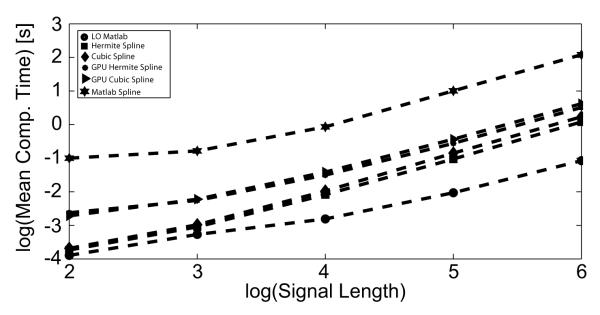
The results of the performance tests are given on Figure 2, Figure 3 and Figure 4. All the tests were performed on a GPU enabled node with 12 CPU cores (2 × Intel Xeon X5680, 3.33GHz processors), 195GB total RAM and a Tesla M2070 GPU with 4GB RAM. Figure 2 shows the mean computational time in seconds as a function of the sequence (signal) length for various implementations in the standalone mode. The tests were performed on one hundred signals with lengths ranging from 10, 10²,…, 10⁶, i.e. input matrices with size 100 × 10, 100 × 100,…, 100 × 10⁶, correspondingly.

Figure 2.

Fractional integration benchmark test: Mean computational time in seconds as a function of the signal length

Figure 3.

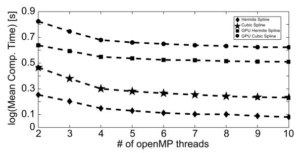
Parallelization benchmark test: Mean computational time in seconds as a function of number of threads

Figure 4.

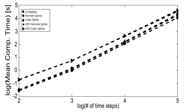
Diffusion simulation benchmark test: Mean computational time in seconds of the diffusion simulations in a standalone mode as a function of the number of time steps

The difference between the best performing implementation- linear-leading order (MATLAB, implicit multithreading) and the cubic spline-leading order+correction(MATLAB, built in cubic spline routine) is three orders of magnitude for signal lengths ~ 10⁶. The increase in computational efficiency comes from the custom implementation of the algorithm [5], the interpolation, as well as the OpenMP multithreading. The difference between the linear-leading order (MATLAB, implicit multithreading) and the more accurate higher order C++ Cubic spline implementation(MEX interface, openMP) is an order of magnitude for signal lengths ~ 10⁶. This makes the employment of accurate higher order methods plausible in the case of fractional dynamical systems simulations.

For any type of numerical integration algorithm it is imperative to quantify the numerical error. In this case we use test functions for which eq.(1.1) results in an explicit expression (f (t) = t, f (t) = t², f (t) = t³ and f (t) = √t). We evaluate the relative error given by

$$RE=\mid \frac{I_{comp}^{\alpha }f\left(t\right)-I_{analytic}^{\alpha }f\left(t\right)}{I_{analytic}^{\alpha }f\left(t\right)}\mid .$$ (3.1)

The results are shown in Table 1.

Table 1.

Relative Error for 10⁴ signal points, α = 0.5

	t	t 2	t 3	√ t
LO	8.96 * 10−16	3.12 * 10−9	7.27 * 10−9	1.32 * 10−7
Cubic	-	8.55 * 10−12	2.98 * 10−11	7.13 * 10−8
Hermite	-	1.29 * 10−11	4.49 * 10−11	7.93 * 10−8
GPUCubic	-	8.55 * 10−12	2.98 * 10−11	7.13 * 10−8
GPUHermite	-	1.29 * 10−11	4.49 * 10−11	7.93 * 10−8
RL Derivative	2.74 * 10−15	3.11 * 10−7	7.76 * 10−7	1.32 * 10−7

The higher order methods outperform the linear leading order implementation in terms of accuracy, justifying the use of spline interpolation for resampling of the interpolation data. Additionally, the integration using splines in High Performance mode is two orders of magnitude faster than the integration using the MATLAB built in spline routine. Thus the use of spline interpolation is feasible for large data sets, which makes sufficiently large real time simulations possible.

Since the FIT supports OpenMP multithreading, it is important to test the scalability of the toolbox. Figure 3 shows the mean performance speed in a standalone mode for the different implementations as a function of the number of openMP threads for 100 input signals of length 10⁶ for the four different implementations. The results (Figure 3) demonstrate a two-fold performance improvement due to multithreading and thus justify the parallelization paradigm employed in the development of the FIT. Depending on available machine configuration (number of processor cores, hyperthreading capability), the user can adjust the number of openMP threads in order to optimize performance.

Another benchmark test we performed is a one dimensional fractional diffusion simulation. Fractional diffusion simulations provide a computational framework for studying anomalous diffusion. Anomalous diffusion plays a significant role in biochemical processes, including molecular signaling in neurons [16], [17]. Figure 4 shows the average computational time for all different implementations in FIT in a standalone mode for a system with 200 spatial points and 10², 10³, 10⁴ and 10⁵ time steps, respectively. At each time step the FIT is called to fractionally integrate the time signal for each space point. All the implementations were numerically stable.

Additional comparison between the standalone (LO) mode and the simulation mode (nested mesh and weight optimization) in a one dimensional fractional diffusion simulation for a system with 200 spatial points and 10⁵ time steps shows performance improvement by a factor of two (not shown).

The results show that for all the implementations in the FIT, one can perform fractional diffusion simulations in real time. Furthermore, due to the independence of time signals in the input matrix, the FIT can be used in any fractional dynamics simulation with no (or minimal) modifications.

References

- 1.Anastasio TJ. The fractional-order dynamics of brainstem vestibulo-oculomotor neurons. Biol. Cybern. 1994;72:69–79. doi: 10.1007/BF00206239. [DOI] [PubMed] [Google Scholar]
- 2.Assaleh K, Ahmad WM. Modeling of speech signals using fractional calculus. 9th International Symposium on Signal Processing and Its Applications, ISSPA 2007, 12-15 Feb..2007. pp. 1–4. [Google Scholar]
- 3.deBoor C. Practical Guide to Splines. Springer; New York: 2001. [Google Scholar]
- 4.Conte SD, deBoor C. Elementary Numerical Analysis. McGraw-Hill; New York: 2002. [Google Scholar]
- 5.Diethelm K, Ford NJ, Freed AD, Luchko Yu. Algorithms for the fractional calculus: A selection of numerical methods. Comput. Methods Appl. Mech. Engrg. 2005;194:743–773. [Google Scholar]
- 6.Diethelm K. The Analysis of Fractional Differential Equations. Springer; Berlin: 2010. [Google Scholar]
- 7.Dokoumetzidis A, Magin R, Macheras P. Fractional kinetics in multi-compartmental systems. J. Pharmacokinet. Pharmacodyn. 2010;37(5):507–524. doi: 10.1007/s10928-010-9170-4. [DOI] [PubMed] [Google Scholar]
- 8.Douglas JF. Some applications of fractional calculus to polymer science. Advances in Chemical Physics. 2007;102:121–191. [Google Scholar]
- 9.Ford NJ, Simpson AC. The numerical solution of fractional differential equations: speed versus accuracy. Numerical Algorithms. 2001;26:333–346. [Google Scholar]
- 10.Fritsch FN, Carlson RE. Monotone piecewise cubic interpolation. SIAM J. Numer. Anal. 1980;17(2) [Google Scholar]
- 11.Melchior P, Orsoni B, Lavialle O, Oustaloup A. The CRONE toolbox for Matlab: Fractional Path Planning Design in Robotics. http://www.ims-bordeaux.fr/CRONE/toolbox.
- 12.Monsrefi-Torbati M, Hammond JK. Physical and geometrical interpretation of fractional operators. J. Franklin Inst. 1998;335B(6):1077–1086. [Google Scholar]
- 13.Nigmatullin RR. Fractional integral and its physical interpretation. Teoret. Mat. Fiz. 1992;90(3):354–368. [Google Scholar]
- 14.Oldham KB, Spanier J. The Fractional Calculus: Theory and Applications of Differentiation and Integration to Arbitrary Order. Dover; Mineola, New York: 2006. [Google Scholar]
- 15.Podlubny I. Geometric and physical interpretation of fractional integration and fractional differentiation. Fract. Calc. Appl. Anal. 2002;5(4):367–386. [Google Scholar]
- 16.Santamaria F, Wils S, de Schutter E, Augustine GJ. Anomalous diffusion in Purkinje cell dendrites caused by spines. Neuron. 2006;52:635–648. doi: 10.1016/j.neuron.2006.10.025. [DOI] [PMC free article] [PubMed] [Google Scholar]
- 17.Santamaria F, Wils S, de Schutter E, Augustine GJ. The diffusional properties of dendrites depend on the density of dendritic spines. Eur. J. Neurosci. 2011;34(4):561–568. doi: 10.1111/j.1460-9568.2011.07785.x. [DOI] [PMC free article] [PubMed] [Google Scholar]
- 18.Sebaa N, Fellah ZEA, Lauriks W, Depollier C. Application of fractional calculus to ultrasonic wave propagation in human cancellous bone. Signal Processing Archive. 2006;86(10):2668–2677. [Google Scholar]
- 19.Soczkiewicz E. Application of fractional calculus in the theory of viscoelasticity. Molecular and Quantum Acoustics. 2002;23:397–404. [Google Scholar]
- 20.Sokolov IM, Klafter J, Blumen A. Fractional kinetics. Physics Today. 2002;55(11):48–54. [Google Scholar]
- 21.Stoer J, Bulirsch R. Introduction to Numerical Analysis. Springer; New York: 1980. [Google Scholar]
- 22.Tepljakov A, Petlenkov E, Belikov J. FOMCON: Fractional-Order Modeling and Control, Toolbox for MATLAB. 18th International Conf. “Mixed Design of Integrated Circuits and Systems”; Gliwice, Poland. Jun 16-18, 2011. [Google Scholar]
- 23.Valerio D, da Costa JS. Ninteger: a non-integer control toolbox for Matlab. http://web.ist.utl.pt/duarte.valerio/FDA04T.pdf.