On the assessment of time-resolved diffraction results

Agreement factors based on the ratio of intensities R collected in dynamic structure pump–probe crystallography experiments are shown to be analogous to the factors widely used in standard crystallographic refinements. Fourier photodifference maps allow the visualization of the externally induced structural changes in the crystal, but also can be used during refinement to monitor its progress. Photodeformation maps are modified to separate the photo-induced structural change from the effect of the temperature increase on laser exposure.

Abstract

Data collected during dynamic structure pump–probe crystallography experiments require appropriate indicators of agreement and tools to visualize the electron-density distribution changes. Agreement factors based on the ratio of intensities R with and without the external perturbation are shown to be analogous to the ₁ and w ₂ factors widely used in standard crystallographic refinements. The η-based factors, normalized by the average relative intensity change, are significantly larger than R-based values. It is shown that the relative intensity change η-based factors are not suitable for comparing different data sets. Fourier photodifference maps allow the visualization of the externally induced structural changes in the crystal, but also can be used during refinement to observe residual peaks not yet accounted for by the model and thus monitor the progress of the refinement. The photodeformation maps are a complementary tool to confirm the validity of the final model. Photodeformation maps with equalized laser-on and laser-off thermal motion are used to highlight the structural changes.

1. Introduction  

Dynamic structure crystallography, and in particular photocrystallography, is a field of great interest because of its numerous applications. The field covers the studies of reactions in crystals including non-reversible reactions, phase transitions and the structural change on excitation leading to short-lifetime species. Such species can serve as light emitters or photosensitizers of semiconductors. Data collected during dynamic structure crystallography experiments require appropriate indicators of agreement and tools to visualize the electron-density distribution changes. The visualization of the externally induced structural changes in the crystal environment is of importance before initiating a structure refinement. It is necessary to check the presence of a structural response and to define a starting point for the structure refinement. In this publication, all the indicators and tools are based on the Ratio method (Coppens et al., 2009 ▶) in which the analysis uses the ratio of the laser-on and laser-off intensities. The method eliminates dependence on the wavelength when using the pink-Laue technique, the need for absorption corrections (Šrajer et al., 2000 ▶; Ren & Moffat, 1995 ▶) and the effect of all but very short-range fluctuations in the source intensity. Indicators of agreement and Fourier difference maps for dynamic structure crystallography previously defined (Coppens et al., 2008 ▶, 2010 ▶) are discussed and complementary new definitions proposed.

2. Agreement factors  

2.1. factors for photocrystallography  

The relative change of intensity of a reflection , , under light exposure is defined as

in which and are, respectively, the laser-on and laser-off intensities, and , the relative intensity under light exposure, is the ratio of the laser-on and laser-off intensities.

In the Ratio method (Coppens et al., 2009 ▶), the refinement of the laser-on structure model is performed against the experimental R ratios while the laser-off model, determined in a prior experiment, is not modified at any refinement step. The calculated ratio of the reflection is defined as the ratio of the calculated squared structure factor with and without light exposure and deduced, respectively, from the laser-on refined model and the laser-off reference model already known:

and the observed ratio, , is the corresponding ratio of the experimental squared structure factors.

The factors for dynamic structure crystallography have been defined by Coppens et al. (2010 ▶), and can be based either on the ratio R values [equation (3)] or on η values [equation (4)]:

In the same way, factors can be adapted and defined based on R [equation (5)] and η values [equation (6)],

in which, for each reflection , = = .

2.2. Comparison with the conventional agreement factors  

In the limiting case in which all structure factors are equal, the R-based and -based factors are similar (Coppens et al., 2010 ▶). It is easier to emphasize this relationship by starting from the factors.

The weighted least-squares (WLS) error function is defined in the Ratio method (Vorontsov et al., 2010 ▶) as follows:

Using equation (2), a semi-experimental estimate of the laser-on squared structure factor, , its standard deviation and the corresponding weight can be defined for each reflection as

Then, the error function can be rewritten as

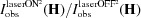
Thus, the R-based (or η-based) WLS minimization is strictly equivalent to an -based WLS minimization. The corresponding factors can be rewritten by combining equations (2) and (8a), (8b) with (5) and (6) to give:

and

Whatever the nature of the used observation, such as intensity I, ratio R or η, if the refined structural model is well defined and the observations and standard deviations properly estimated, the function should follow at the convergence of the model a -distribution function with degrees of freedom, with N the number of observations and V the number of model variables. This implies that its expected value is equal to and the corresponding goodness-of-fit factor will tend to 1.0. Thus, the range of values of these factors will accordingly only depend on the definition of their denominators.

The quantity of interest in the R-based factor is in its original definition [equation (5)], the ratio R, and in its rewritten expression [equation (10)], which is similar to an -based factor, the semi-experimental estimates of the laser-on diffraction intensities. In the following we examine the relation between expressions of the R-based [equation (5)] and -based factors. Assuming and , Coppens et al. (2010 ▶) deduce from the theory of error propagation:

which can be rewritten by dividing by the factor = :

assuming

It follows that the denominator of the R-based factor [equation (5)] is related to the -based -factor denominator:

and thus, considering that the numerators of the R-based [equation (5)] and -based factors should tend to 1.0 while their denominators differ,

A range of values larger but of the same order as the -based factors can be expected for the R-based factors (Coppens et al., 2010 ▶).

On the other hand, the η-based factor cannot be rewritten as a -based one. Its distinct denominator is the weighted quadratic mean of the η values in its original definition [equation (6)], or of the difference − in its rewritten expression [equation (11)]. Thus, the η-based factor is normalized by the average change in intensity rather than the average intensity. In photocrystallography studies, we usually expect to observe excited-state structural changes with small conversion populations to preserve crystal sample integrity, which means the diffraction signal change would be small relative to the absolute diffraction signal. For this reason, the η-based factor will have larger values than the R-based ones. Furthermore, the light-induced changes in the observed intensities consist of two contributions: the light-induced structural conformation changes and the increase of the thermal atomic displacements. The latter become dominant when the laser exposure results in significant heating of the sample, resulting in an increase in the η-based denominator and therefore a decrease in the values of η-based factor. This interferes with the validity of using this R factor in comparing the refinement of different data sets.

3. Difference maps  

The dynamic factors can be easily monitored during the refinement of the laser-on structure model using the software LASER (Vorontsov et al., 2010 ▶) thus allowing step-by-step following of the improvement of the refinement model. However, by definition, the agreement factors do not provide any information about the validity of the refined structure, as a model with a large number of parameters can minimize any factors. An additional analysis tool more suitable for evaluation of the model is required. Fourier difference maps can serve this purpose.

3.1. Prior-refinement photodifference maps  

Difference Fourier maps have been used in our previous studies of molecular excited states (Makal et al., 2011 ▶; Collet et al., 2012 ▶; Coppens et al., 2008 ▶), but for a more restricted purpose than proposed here. All difference Fourier maps share a common general formula:

The photodifference map referred to here as type A has proved to be useful in the previous studies. It is based on the laser-on and laser-off sets of experimental structure factors. Moreover, the phases of the experimental laser-on and laser-off structure factors are assumed equal to the calculated laser-off phases deduced from the structure model refined against an independent data set of optimal quality, preferably collected with monochromatic radiation. This assumption is most appropriate for centrosymmetric structures when conversion percentages are low. In this case, the Fourier summation, equation (16), can be rewritten as follows:

In the particular case of the Ratio method (Coppens et al., 2009 ▶), the observations collected during the pump–probe experiments are the ratios R of laser-on and laser-off intensities for each reflection . Then, the experimental laser-on and laser-off absolute structure factors are expressed for each reflection as:

with the scale factor refined during the refinement of the reference laser-off structure model against the independent data set.

Finally, the laser-off phase is deduced from the reference laser-off model obtained from the same independent diffraction experiment. The photodifference type A expression becomes, using equations (18a), (18b),

Both the laser-on and laser-off structure factors depend on experimental data and thus the residual features will be related to the light-induced changes, although obviously affected by the use of laser-on and laser-off calculated phases, assumed to be equal, data quality and Fourier series truncation.

3.2. Residual maps  

Fourier residual maps are an essential tool in structural and charge-density distribution refinements. In the case of photocrystallography analogous residual maps can be used to confirm the reliability of the model definition and monitor the progress of the refinement.

The least-squares function minimized in the Ratio method is based on the ratio R values but can be rewritten as an -based function as in equation (9). The corresponding difference map, referred to as type B, is defined as:

The type B residual map can be calculated at any refinement step using the laser-on refined structure model obtained at that stage.

The residual map can also be used prior to any laser-on structure model refinement as a photodifference map by substituting the reference laser-off structure model as the initial laser-on model. In that case, the absolute laser-off structure factor can be factored as follows:

It may be noted that the factored expressions of the type A [equation (19)] and type B [equation (21)] photodifference maps are very similar.

3.3. Calculated photodeformation maps  

In high-resolution crystallography, the data quality and resolution allow modeling the non-spherical atomic electron-density distribution. It is common use to illustrate the electron accumulation/depletion by visualizing the difference of the electron-density distributions calculated from the non-spherical model and the corresponding spherical independent atom model (IAM). These maps are referred to in the literature as electron-density deformation maps (Hirshfeld, 1971 ▶; Harel & Hirshfeld, 1975 ▶). In the same vein, we define photodeformation maps which show the light-induced changes representing the difference between the laser-on and reference laser-off IAM electron-density distributions. These deformation maps are calculated with equation (22):

They can be evaluated at different resolution limits. When a full sphere of reflections and/or a different resolution are used, they cannot be compared directly with the more limited experimental maps. To highlight the effect of the structural changes, the effect of a temperature increase in the laser-on IAM can be eliminated by setting the parameter to 1.0, which equates the thermal parameters of the laser-on and laser-off densities. The parameter is used in the program LASER to refine the increase of the thermal effects assuming a proportionality between the laser-on and laser-off atomic displacement parameters such that for all atoms.

4. Application and discussion  

Application of the factors and the difference maps will be illustrated with the case of the α-polymorph of Rh₂(μ-PNP)₂(PNP)₂.BPh₄ where PNP = CH₃N(P(OCH₃)₂)₂ and Ph = phenyl, and referred later to as RhPNP (Makal et al., 2011 ▶). RhPNP crystallizes in the space group with cell parameters a = 13.9783 (3), b = 20.2046 (5) and c = 28.1465 (7) Å and β = 90.8420 (10)°.

4.1. Synchrotron data collection for RhPNP  

Makal et al. (2011 ▶) performed the refinement of the laser-on structure model using the program LASER (Vorontsov et al., 2010 ▶). Time-resolved single-crystal Laue X-ray data were collected on the 14-ID BioCARS beamline at the Advanced Photon Source. For the current study, each raw frame data set has been reprocessed using the last version of the toolkit LaueUtil (Kalinowski et al., 2011 ▶, 2012 ▶) and subsequently analyzed and merged with the program SORTAV (Blessing, 1997 ▶) to improve the quality and completeness. The joint refinement of the RhPNP model under light exposure was performed using the same structural model and refinement program as Makal et al. (2011 ▶), but against the six partial newly processed R data sets and using a random distribution (RD) model of the excited-state compounds.

To calculate a physically correct Fourier difference map, a complete data set is necessary. In practice, this is difficult to achieve in pump–probe experiments. It is a frequent occurrence in data collection with the laser-pump X-ray probe technique that crystals disintegrate before a full data set can be collected. To gain in completeness, it is possible to merge the partial data sets measured on different samples. However, different experimental settings such as pump–probe delay, laser pulse width or power may have been used, and also the samples do not generally share the same size, mosaicity and orientation. For these reasons, a scaling procedure is strongly recommended. In the current study scaling was performed for each merged data set i by multiplying the η values of individual reflections by with, respectively, and the average absolue η values over all measured reflections and over the reflections in the specific data set i (Schmøkel et al., 2010 ▶; Makal et al., 2011 ▶).

The six partial data sets used are described and the corresponding scaling factor values are specified in Table 1 ▶.

Table 1. Description of the data sets.

Data set	No. of unique reflections	Completeness (%)	Maximal resolution (Å−1)	Undulator setting (keV)	Laser power (mJ mm−2)
19	1813	35.90	0.423	12	0.60	−0.0313	0.0491	1.165
20	1210	24.30	0.419	12	0.60	−0.0648	0.0799	0.717
24	1116	21.80	0.424	12	0.55	−0.0732	0.0891	0.642
27	1453	15.30	0.522	15	0.45	−0.0367	0.0561	1.020
28	2668	27.60	0.525	15	0.45	−0.0248	0.0484	1.182
29	2440	24.30	0.532	15	0.45	−0.0217	0.0477	1.199

After applying the scaling procedure, the ratio R values of all reflections are merged with the program SORTAV (Blessing, 1997 ▶). The merged data set obtained counts 4008 unique reflections for a completeness of 39.9%.

4.2. -factor values at the end of the structural refinement  

The behavior of the laser-on structural model has been monitored during the progress of the joint refinement using the four different factors (see §2.1 for definitions). The final values of the indicators of quality are provided per data set in Table 2 ▶ with their thermal scale factor (see §3.3 for the definition).

Table 2. -factor values and parameters for each data set used in the joint refinement of the compound RhPNP.

Data set
19	0.0316	0.6227	0.0254	0.5112	1.0786
20	0.0388	0.4541	0.0333	0.3929	1.1684
24	0.0436	0.4536	0.0375	0.4010	1.1969
27	0.0399	0.6854	0.0304	0.5572	1.0717
28	0.0364	0.7329	0.0271	0.5765	1.0582
29	0.0359	0.7360	0.0279	0.6261	1.0483

As expected, according to the preceding discussion (see §2.2), the η-based factors have larger values than the R-based ones. The R-based factors have a similar range of values to the conventional ones, while the -based factors, normalized by the average relative intensity change, have a range of values larger by one order of magnitude.

The plot of the η-based -factor values (Fig. 1 ▶) shows a decrease with increasing values. This dependence is expected considering the η-based -factor definitions [equations (4), (6)]. The increase of the thermal effect leads to the increase of the number of negative η. Then, the arithmetic average absolute η, , and the quadratic weighted average absolute η, , respectively, denominators of and , become larger, leading to a decrease of these indicators. Conversely, the R-based -factor values show a weak tendency to increase with the values (Fig. 1 ▶). This tendency may be attributed to the correlation between the different and R-based factors resulting from the joint refinement being performed using the program LASER (Vorontsov et al., 2010 ▶; Schmøkel et al., 2010 ▶).

Figure 1.

-factor values for the different data sets plotted against the corresponding . The top figure shows the plot of the η-based values with as blue filled circles and as blue open circles, and the lower figure the R-based values with as red filled squares and as red open squares. Note the difference between the vertical scales of the two plots. Plots made using the program GNUPLOT (Williams & Kelley, 2010 ▶).

4.3. Prior refinement photodifference maps  

As expected, the photodifference maps type A (Fig. 2 ▶ a) and type B (Fig. 2 ▶ b) calculated prior to the refinement are in very good agreement. Their discrepancies are not detectable in the figures.

Figure 2.

Photodifference maps type A (a) and type B (b) with isosurfaces (blue positive, red negative) of 0.25 e Å⁻³. Maps calculated with the program OLEX2 (Dolomanov et al., 2009 ▶).

Only the nature of the laser-off structure-factor amplitude, experimental or calculated, changes in the expressions of the maps type A and B [equations (19), (21)]. This implies the Fourier series of the photodifference maps type A and B share the same phases. Moreover, the monochromatic data set used to refine the laser-off IAM has better statistics than the ratio data set especially with its completeness of 97.2% and its resolution limit of 0.6450 Å⁻¹. Thus, the disagreement between the observed and calculated structure-factor amplitudes of the reference data set is relatively minor.

4.4. Residual maps for validation of refined models  

The residual map calculated using the refined laser-on model obtained by joint refinement against all data sets, and the scaled/merged data set requires a supplementary step. This step consists of refining exclusively the excited-state (ES) population P and the thermal factor of the laser-on structure model against the scaled/merged data set. The residual maps type B are calculated and illustrated (Fig. 3 ▶) at an isomesh level of 0.15 e Å⁻³. The residual map (Fig. 3 ▶ a) is obtained after a partial model refinement, considering only the Rh-atom positions and data-set variables (, population P). Positive peaks are visible in the vicinity of the Rh atoms. Residual peaks can be seen near the P atoms too, and even for two of them positive/negative dipole-like features, which supports the refinement of position/orientation of the PNP chemical moieties.

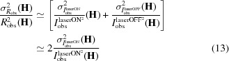
Figure 3.

Residual maps type B (a) after refinement of Rh-atom positions and data-set variables (, P) and (b) after refinement of all model parameters adding the position/rotation variables of the four PNP rigid bodies, with isosurfaces of 0.15 e Å⁻³. Maps calculated with the program OLEX2 (Dolomanov et al., 2009 ▶).

The residual map (Fig. 3 ▶ b) is obtained after the complete refinement of the model defined by Makal et al. (2011 ▶) which considers the two Rh atoms as independent atoms and the four PNP moieties as rigid bodies. Only two elongated and almost parallel peaks are visible on the left sides of each of the Rh atoms plus a density feature on Rh2, indicating the improvement in the model.

4.5. Photodeformation maps  

As explained in §3.3, photodeformation maps based on the model parameters and calculated by inverse Fourier transform allow selection of a partial set of hkl indices for direct comparison with the photodifference maps. Several photodeformation maps computed considering different sets of hkl are illustrated (Fig. 4 ▶).

Figure 4.

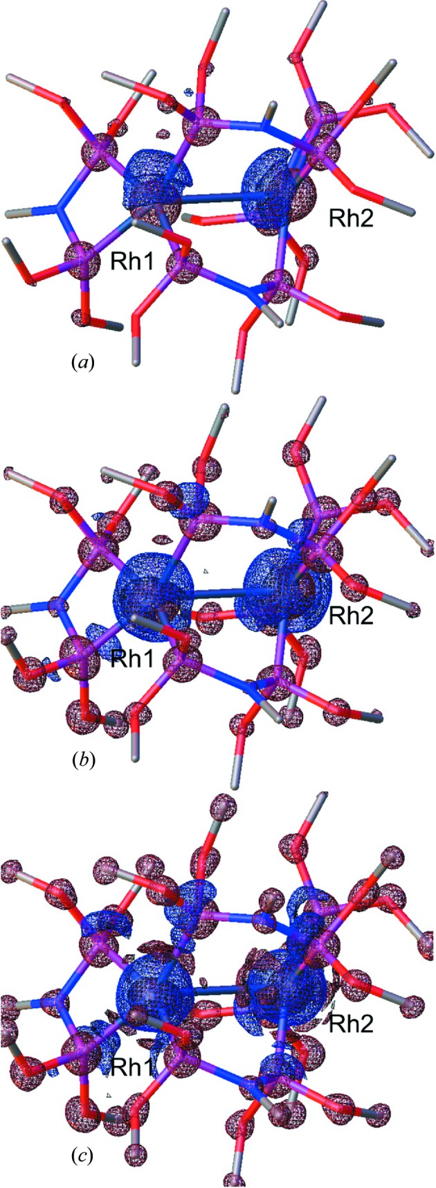
Three-dimensional photodeformation maps of electron-density distribution with isosurfaces (blue positive, red negative) of 0.25 e Å⁻³. Maps obtained using the hkl set of the merged ratio data set (a), using all hkl with maximal resolution 0.5317 Å⁻¹ (b) and 0.6450 Å⁻¹ (c). Illustrations made using the program OLEX2 (Dolomanov et al., 2009 ▶).

The first map (Fig. 4 ▶ a ▶) is calculated based on the same set of hkl indices as the merged ratio data set and illustrated with the same isomesh level of 0.25 e Å⁻³ as the experimental photodifference maps (Fig. 2 ▶). This photodeformation map globally agrees with the photodifference maps type A and B. Similar large positive peaks localized near the Rh atoms can be noticed, although the Rh1-atom peak embeds the atom less. The two other maps (Figs. 4 ▶ b and 4 ▶ c) are calculated with complete sets of hkl with, respectively, the same resolution limit as the ratio data set (0.5317 Å⁻¹) and that of the monochromatic reference data set (0.6450 Å⁻¹). Comparing Figs. 4 ▶(a) and 4 ▶(b) illustrates how the dramatic increase of the completeness from 40% to 100% reveals more details. The strong positive deformation peaks almost completely enclose the Rh atoms while the positive peaks near the P atoms resulting from their translations on excitation become clearly visible. Extra negative peaks, related to the thermal effect, are observed on the lighter atom (N and O) positions especially at the highest resolution of 0.6450 Å⁻¹.

The enhancement of localized electron concentrations/depletions with the increase in completeness and resolution limit of the hkl set is also visible in the two-dimensional photodeformation maps made in the plane of the two Rh atoms and the P4 atom (Fig. 5 ▶).

Figure 5.

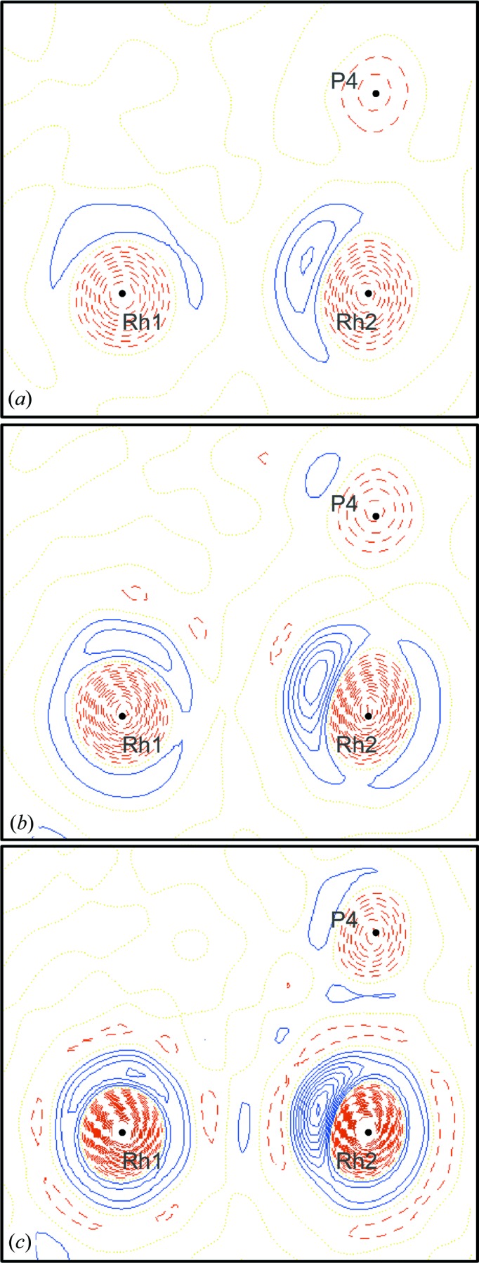
Two-dimensional photodeformation maps of electron-density distribution in the plane of the Rh1, Rh2 and P4 atoms. Drawn with an isocontour step of 0.20 e Å⁻³, positive isocontours in blue solid lines, negative in red dashed lines and neutral in yellow dot lines. Map obtained using the hkl set of the merged ratio data set (a), using all hkl with maximal resolution 0.5317 Å⁻¹ (b) and 0.6450 Å⁻¹ (c). Illustrations made using the program XD2006 (Volkov et al., 2006 ▶).

As in the three-dimensional maps, the positive deformation peaks of the Rh atoms become larger and a positive peak of the P4 atom becomes visible with the improvement of the completeness (Fig. 5 ▶ b). Spherical-like shells of positive electron density become increasingly visible around both Rh atoms when the resolution increases (Fig. 5 ▶ c).

The deformation shells surrounding the Rh atoms result from the temperature increase. The lack of sphericity of these shells is mostly due to the atomic shift of the Rh atoms on excitation. This is confirmed by the photodeformation maps calculated after setting the thermal factor to 1.0 and considering the same set of hkl as the merged ratio data set (Fig. 6 ▶ a) or the set of hkl with a full completeness and the same resolution limit as the monochromatic data set (Fig. 6 ▶ b). Dipole deformation features can be seen on these equal-temperature photodifference maps. Extra dipoles become visible with the gain in completeness and resolution (Fig. 6 ▶ b). The axis of each observed dipole matches the direction of the corresponding atomic shift (Fig. 6 ▶ c).

Figure 6.

Photodeformation maps eliminating the thermal increase by setting to 1.0 and considering the same set of hkl as the merged ratio data set (a) and a full set of hkl with a resolution limit of 0.6450 Å⁻¹ (b), with isosurfaces (blue positive, red negative) of 0.15 e Å⁻³ visualized with the program OLEX2 (Dolomanov et al., 2009 ▶). Illustration of the RhPNP conformations (c) with ground state in blue and excited state in red visualized with the program PyMOL (DeLano Scientific, 2009 ▶).

The extended resolution photodeformation maps highlight the value of a gain in experimental resolution. This was not possible for instrumental reasons in the RhPNP experiment, but is highly desirable in future experimental studies.

5. Conclusion  

The and factors widely used in standard crystallographic refinements can be calculated based on the ratio of intensities R or the relative intensity difference η for dynamic crystallographic studies especially photocrystallography. factors based on R values tend to be of the same order as conventional -based ones. The η-based factors, normalized by the average relative intensity, are significantly larger than R-based ones. Their range of values is even of a different order of magnitude in the example provided in this paper. The η-based factors are not suitable for comparison of refinements against different data sets. Fourier photodifference maps allow the visualization of the externally induced structural changes in the crystal, but also can be used during refinement to observe residual peaks not yet accounted for by the model. The photodeformation maps are a complementary tool to confirm the validity of the final model.

References

- Blessing, R. H. (1997). J. Appl. Cryst. 30, 421–426.
- Collet, E., Moisan, N., Balde, C., Bertoni, R., Trzop, E., Laulhe, C., Lorenc, M., Servol, M., Cailleau, H., Tissot, A., Boillot, M.-L., Graber, T., Henning, R., Coppens, P. & Cointe, M. B.-L. (2012). Phys. Chem. Chem. Phys. pp. 6192–6199. [DOI] [PMC free article] [PubMed]
- Coppens, P., Kamiński, R. & Schmøkel, M. S. (2010). Acta Cryst. A66, 626–628. [DOI] [PubMed]
- Coppens, P., Pitak, M., Gembicky, M., Messerschmidt, M., Scheins, S., Benedict, J., Adachi, S., Sato, T., Nozawa, S., Ichiyanagi, K., Chollet, M. & Koshihara, S. (2009). J. Synchrotron Rad. 16, 226–230. [DOI] [PMC free article] [PubMed]
- Coppens, P., Zheng, S.-L. & Gembicky, M. (2008). Z. Kristallogr. 223, 265–271.
- DeLano Scientific (2009). The PyMOL Molecular Graphics System, version 1.2r2. Schrödinger, LLC.
- Dolomanov, O. V., Bourhis, L. J., Gildea, R. J., Howard, J. A. K. & Puschmann, H. (2009). J. Appl. Cryst. 42, 339–341.
- Harel, M. & Hirshfeld, F. L. (1975). Acta Cryst. B31, 162–172.
- Hirshfeld, F. L. (1971). Acta Cryst. B27, 769–781.
- Kalinowski, J. A., Fournier, B., Makal, A. & Coppens, P. (2012). J. Synchrotron Rad. 19, 637–646. [DOI] [PMC free article] [PubMed]
- Kalinowski, J. A., Makal, A. & Coppens, P. (2011). J. Appl. Cryst. 44, 1182–1189. [DOI] [PMC free article] [PubMed]
- Makal, A., Trzop, E., Sokolow, J., Kalinowski, J., Benedict, J. & Coppens, P. (2011). Acta Cryst. A67, 319–326. [DOI] [PMC free article] [PubMed]
- Ren, Z. & Moffat, K. (1995). J. Appl. Cryst. 28, 482–494.
- Schmøkel, M. S., Kamiński, R., Benedict, J. B. & Coppens, P. (2010). Acta Cryst. A66, 632–636. [DOI] [PubMed]
- Šrajer, V., Crosson, S., Schmidt, M., Key, J., Schotte, F., Anderson, S., Perman, B., Ren, Z., Teng, T., Bourgeois, D., Wulff, M. & Moffat, K. (2000). J. Synchrotron Rad. 7, 236–244. [DOI] [PubMed]
- Volkov, A., Macchi, P., Farrugia, L. J., Gatti, C., Mallinson, P. R. & Richter, T. K. T. (2006). XD2006 – a computer program package for multipole refinement, topological analysis of charge densities and evaluation of intermolecular energies from experimental and theoretical structure factors. State University of New York at Buffalo, Buffalo, NY 14260-3000, USA.
- Vorontsov, I., Pillet, S., Kamiński, R., Schmøkel, M. S. & Coppens, P. (2010). J. Appl. Cryst. 43, 1129–1130.
- Williams, T. & Kelley, C. (2010). GNUPLOT An interactive plotting program, version 4.4. Duke University, Durham, NC, USA.