Abstract
A new approach based on nonlinear inversion for autocalibrated parallel imaging with arbitrary sampling patterns is presented. By extending the iteratively regularized Gauss–Newton method with variational penalties, the improved reconstruction quality obtained from joint estimation of image and coil sensitivities is combined with the superior noise suppression of total variation and total generalized variation regularization. In addition, the proposed approach can lead to enhanced removal of sampling artifacts arising from pseudorandom and radial sampling patterns. This is demonstrated for phantom and in-vivo measurements.
Keywords: Parallel Imaging, Radial Sampling, Pseudorandom Sampling, Nonlinear Inversion, Total Variation, Total Generalized Variation
INTRODUCTION
It was shown recently (1-4) that nonlinear inversion can be applied successfully to image reconstruction of undersampled data from multiple coils, i.e., parallel imaging (5-7). The joint estimation of images and coil sensitivities, which can be achieved with an iteratively regularized Gauss–Newton (IRGN) method, leads to more accurate estimation of the coil sensitivities, and therefore yields results with improved image quality. It was also demonstrated that this method can be extended to non-Cartesian imaging (8,9). In particular, radial sampling has the advantage that the sampling pattern automatically leads to an oversampling of the central frequencies of k-space, which eliminates the need to acquire additional reference lines when performing auto-calibrated parallel imaging. Another important characteristic of radial sampling is the fact that aliasing artifacts, which are introduced by under-sampling, have a distinctively regular appearance which is usually different from the image content. For this reason, it is possible to remove these so-called streaking artifacts during reconstruction with the integration of suitable penalties on the reconstructed image, with total variation (TV) proving particularly effective in the radial case (10,11). Successful application of TV regularization to conventional Cartesian subsampling had been reported as well (12). This interest in total variation-type regularization has been stimulated by the success of compressed sensing (13, 14) in MRI (15-17), which is often used in combination with pseudorandom sampling (i.e., randomly selecting sampling points from a regular Cartesian grid); see also (18) for a related idea. Recently, compressed sensing has also been used for parallel imaging with unkown coil sensitivies by formulating the reconstruction as a low-rank matrix completion problem (19).
The purpose of this work is to demonstrate that the formulation of autocalibrated parallel imaging as a nonlinear inverse problem yields a general framework that allows the joint estimation of coil sensitivities and image content in combination with arbitrary sampling patterns and variational penalties. This is illustrated via the integration of a TV penalty in the IRGN method. The immediate benefit is that TV regularization helps to suppress the noise amplification (20) that seriously limits parallel imaging with conventional methods (for linear reconstruction methods, the effect of noise suppression due to regularization is well known (21-24)). When applied to data sets obtained with radial or pseudorandom sampling patterns, TV also leads to enhanced removal of artifacts. The flexibility is further shown by replacing TV with a different convex regularization functional that is more suitable in cases when the assumption of piecewise constant images is not reasonable: total generalized variation (TGV) of second order (25,26). A similarly general approachin terms of sampling patterns and variational penalties is followed in SPIRiT (27), which can also be formulated as a nonlinear minimization problem. In contrast to the approach considered here, calibration is carried out in a separate step, and the corresponding variant with non-quadratic regularization (L1 SPIRiT) is based on compressed sensing using a wavelet transform.
THEORY
Mathematically, parallel MR imaging can be formulated as a nonlinear inverse problem where the sampling operator (defined by the k-space trajectory, e.g., Fourier transform followed by multiplication with a binary mask in the case of standard Cartesian subsampling) and the correspondingly acquired k-space data g = (g1, …, gN)T from N receiver coils are given, and the spin density u and the unknown (or not perfectly known) set of coil sensitivities c = (c1, …, cN)T have to be found such that
| [1] |
holds. As was shown in (3, 8), this problem can be solved using the iteratively regularized Gauss–Newton (IRGN) method (28-31), i.e., computing in each step k for given xk:= (uk, ck) the solution δx:= (δu, δc) of the minimization problem
| [2] |
for given αk, βk > 0, and then setting xk+1:= xk + δx, αk+1 := qα αk and βk+1 := qβ βk with 0 < qα, qβ < 1. Here, F′(xk) is the Fréchet derivative of F evaluated at xk. The term is a penalty on the high Fourier coefficients of the sensitivities and is a regularization term for the image. So far, the application of the IRGN method to parallel imaging has been formulated with a conventional L2 penalty (3,8) (i.e., ). As demonstrated in this work, the IRGN method can also be used with other regularization terms, which can be chosen dependent on the application. For example, the stability of the method with respect to noise can be improved: Since αk and βk are decreasing during the iteration, the problem in Eq. 2 will become increasingly ill-conditioned. This leads to noise amplification, which can be counteracted by using a regularization term with stronger noise removal properties than the L2 penalty. A possible choice is the total variation (TV) of the image, i.e.,
| [3] |
 |
where |·|2 denotes the Euclidean norm in . To calculate the solution of Eq. 2, we make use of the dual characterization of the TV semi-norm:
| [4] |
where p = (p1, p2)T, div p = ∂xp1 + ∂yp2 with appropriate boundary conditions and
| [5] |
The problem in Eq. 2 then becomes a non-smooth convex-concave saddle-point problem,
| [6] |
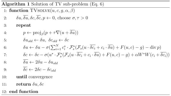
which can be solved efficiently using a projected primal-dual extra-gradient method (32,33), given as Algorithm 1. Since this requires only application of F′(xk) and its adjoint F′(xk)*, the algorithm can be implemented efficiently on modern multi-core hardware such as graphics processing units (GPUs). Due to the bilinear structure of F, the action of F′(xk) and F′(xk)* can be calculated explicitly in terms of the subsampling operator and its adjoint . The projection onto the convex set Cβ can be calculated pointwise by setting for all x ∈ Ω
| [7] |
Since TV regularization is known to introduce staircasing artifacts if the penalty parameter is large, we also consider second order total generalized variation (TGV),
 |
which is a generalization of TV that avoids the staircasing in regions of smooth signal change (25,26). This amounts to setting
| [8] |
where denotes the symmetrized gradient of the complex-valued vector field . We refer to (25, 26) for a detailed description of this functional and an explanation of its properties. Using again the dual representation of the norms, the Gauss–Newton step (Eq. 2) is equivalent to the saddle point problem
| [9] |
where
| [10] |
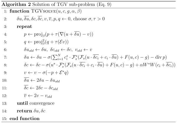
and denotes the set of symmetric complex matrices. The corresponding extragradient method is given as Algorithm 2, where the projection onto can again be computed pointwise.
MATERIALS AND METHODS
Data Acquisition
Experiments were performed for 3D pseudorandom as well as 2D radial sampling patterns. All measurements were performed on a clinical 3T system (Siemens Magnetom TIM Trio, Erlangen, Germany). Written informed consent was obtained from all volunteers prior to the examination.
Accelerated acquisition with pseudorandom sampling was tested with phantom experiments. A receive-only 12-channel head coil was used, and an SVD based coil compression (34) was applied to reduce the data to 8 virtual channels. Measurements were performed with a 3D FLASH sequence with the following sequence parameters: TR=20ms, TE=5ms, flip angle 18°, matrix size 256×256×256. The pulse sequence was modified to include a binary 2D mask defining the subsampling of both phase-encoding directions. A resolution of 1mm×1mm×5mm was used. Raw data was exported from the scanner, a 1D Fourier transform was performed along the readout direction, and partitions orthogonal to this axis were reconstructed.
Additionally, a fully sampled T2 weighted 2D turbo spin echo data set of the brain of a healthy volunteer was acquired with a 32-channel receive coil. The data was compressed to 12 virtual channels. Sequence parameters were TR=5000ms, TE=99ms, turbo factor 10, matrix size 256×256, slice thickness 4mm and an in-plane resolution of 0.86mm×0.86mm. Raw data was exported from the scanner and then subsampled retrospectively with an adapted pseudorandom sampling pattern (16), where sampling points on a regular Cartesian grid are randomly selected according to a specified probability density function which is based on the energy distribution in k-space of medical images (35).
For comparison, conventional TV filtering was applied to the magnitude images obtained from standard IRGN reconstruction of the T2 weighted data set of the brain. This experiment was repeated for an accelerated pseudorandom in-vivo measurement of the brain of a different volunteer. The same experimental setup was used as in the accelerated phantom experiments, except that 9 SVD compressed virtual channels were used and an isotropic spatial resolution of 1mm was achieved.
Radial sampling experiments were performed with an rf-spoiled radial FLASH sequence with sequence parameters TR=2.0ms, TE=1.3 ms, and a flip angle of 8°. Images of a water phantom and of the heart of a healthy volunteer were made. Invivo data was acquired with a 32-channel body array coil, and data acquisition was performed with a protocol designed for real-time imaging (36-38) without cardiac gating and during free breathing (39). After the acquisition, the data was compressed to 12 virtual channels for the in-vivo experiments and 8 virtual channels for the phantom experiments. An in-plane resolution of 2mm×2mm and a slice thickness of 8mm was used in combination with 128×128 image matrices. Due to the two-fold oversampling, this resulted in 256 sample points for each radial spoke.
Nonlinear reconstruction
All reconstructions were performed offline using a Matlab (R2010a, The MathWorks, Natick, MA, USA) implementation of the described nonlinear inversion method. For the reconstruction of radial data sets, Fessler and Sutton’s NUFFT (40) code was used. To facilitate comparison, the solution of Eq. 2 with was computed using the same extra-gradient scheme, which can be obtained from Algorithm 1 by removing step 4 and replacing the term − div p with in step 6. In the following, we will refer to the Gauss–Newton reconstruction using an L2-penalty simply as IRGN, while the reconstruction using TV and TGV penalties will be denoted by IRGN-TV and IRGN-TGV, respectively.
Parameter Choice
The parameters in Algorithm 1 were chosen according to the convergence theory for the projected extra-gradient scheme. The step lengths σ and τ were selected such that στL2 < 1 holds, where L is the Lipschitz constant of the gradient of the functional to be minimized. This constant depends on the subsampling strategy and the iterates uk, ck, but can be estimated using a few iterations of the power method to approximately compute the norms of the partial Fréchet derivatives of the linearized operator F′(x). As the norm of the finite difference approximation of the divergence and gradient operators with mesh size 1 is , we set in Algorithm 1, where , are the estimates from the power method. The step lengths in Algorithm 2 were set to based on the norm of the linear operator involving the symmetrized derivative. The iteration was terminated after a fixed number of iterations, since the efficiency estimate for the extra-gradient method gives an upper bound on the required number of iterations to achieve a given accuracy. Since a high accuracy is not necessary during the initial Gauss–Newton iterations with large penalties, we started with N0 = 20 iterations and set Nk = 2Nk+1. These choices were stable and yielded good results for all data sets.
The parameters in the Gauss–Newton iteration were chosen according to a quasioptimality criterion. The initial penalties α0, β0 were chosen such that the norm of the residual ||F (u1, c1) − g|| after the first iteration was roughly 3/4 of the initial residual, and the reduction factors qα, qβ were set such that each further iteration roughly reduced the residual by a factor of 1/2. The iteration was terminated once the achieved reduction factor fell below 3/4. This lead to the choice α0 = 1, β0 = 2, qα = qβ = 1/10, and 5 Gauss–Newton iterations for the radial data set. For the pseudorandom data set, β0 = 1, qβ = 1/5 and 6 Gauss–Newton iterations were used.
Since the TV regularization parameter is continually decreased during the Gauss–Newton iteration, the final reconstruction will typically not show strong signs of TV filtering such as a cartoon-like appearance. A more pronounced TV effect can be achieved if the decrease of the regularization parameter is stopped at the desired level. To illustrate this, we will also show reconstructions where we have set βk+1 = max(βmin, qβ βk) with βmin = 5 · 10−3 for L2, TV and TGV regularization (with otherwise unchanged parameters).
Due to the difference in functionals and normalization of raw data and reconstructed magnitude images, it is not sensible for comparison purposes to use the above values of βmin as regularization parameters for TV filtering. Instead, based on visual inspection, an optimal parameter was chosen for each data set. For the subsampled data with R = 6, this was , while the accelerated in-vivo data with R = 4 required .
RESULTS
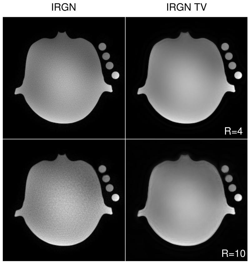
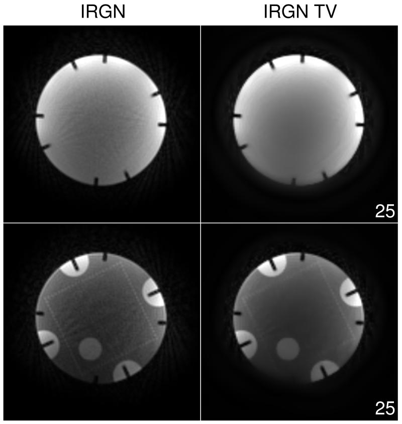
Figure 1 shows a partition of a water phantom reconstructed with IRGN and IRGN-TV from pseudorandomly subsampled 3D data using acceleration factors R = 4 and R = 10. The reduced noise amplification and artifact removal characteristics of IRGN-TV are clearly visible for both acceleration factors. In the case of moderate acceleration with R = 4, the final TV regularization parameterβmin was set to zero. For R = 10, βmin = 5 · 10−3 was used to achieve a stronger TV regularization and a better removal of artifacts. It must be noted that the phantom only consists of regions that are piecewise constant, and therefore the underlying assumption of the TV penalty is fulfilled. However, in the case of R = 10 with increased TV regularization, staircasing artifacts can be observed in regions where modulations caused by the inhomogeneity of the coil sensitivities affect the reconstructed image.
Figure 1.
Comparison of IRGN (left) and IRGN-TV (right) for pseudorandom subsampling of a water phantom. Top: acceleration factor R = 4, βmin = 0; bottom: R = 10, βmin = 5 · 10−3.
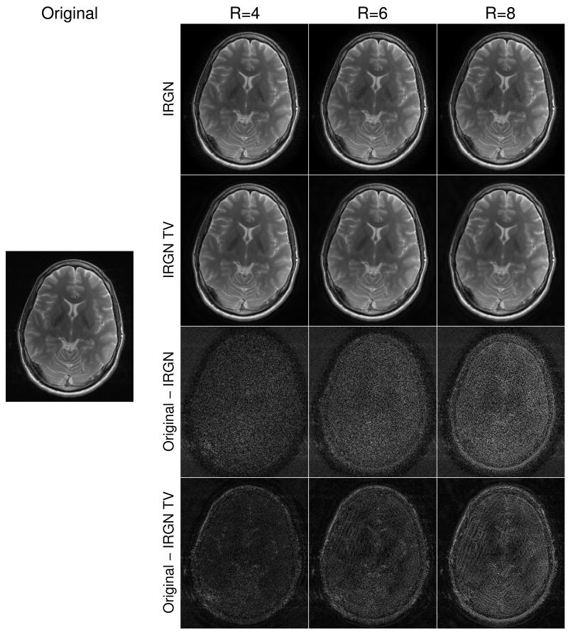
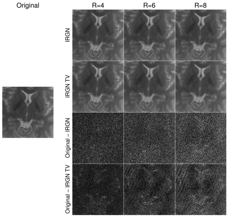
The above findings are confirmed for in-vivo conditions. IRGN and IRGN-TV reconstructions (with βmin = 0) of the retrospectively pseudorandomly subsampled T2 weighted data of the brain are displayed in Fig. 2, together with a sum-of-squares image obtained from the fully sampled data. Shown are results for acceleration factors of R = 4, R = 6 and R = 8 (defined as the ratio of total to acquired points on the underlying Cartesian sampling grid) as well as difference images to the fully sampled SOS image. With larger acceleration factors, an increasing amount of noise amplification and residual incoherent aliasing can be observed in the IRGN reconstructions, while this effect is reduced with IRGN-TV. The difference is especially noticeable in the magnified details shown in Fig. 3.
Figure 2.
Comparison of IRGN (first row) and IRGN-TV (second row) for retrospective pseudorandom subsampling (βmin = 0). From left: fully sampled acquisition, acceleration factors R = 4, R = 6, R = 8. difference images to the fully sampled SOS reconstruction are shown for IRGN (third row) and IRGN-TV (fourth row) and are rescaled individually for IRGN and IRGN-TV to allow better depiction of the pixel differences.
Figure 3.
Magnified detail of Figure 2.
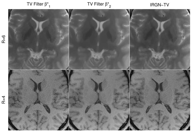
The comparison of IRGN-TV with IRGN followed by TV filtering of the reconstructed magnitude image is shown in Fig. 4. The conventional IRGN reconstruction of the T2 weighted brain data with R = 6 (see Fig. 2) was postprocessed with a TV filter, where an optimal TV parameter was chosen based on visual inspection. To illustrate the robustness of IRGN-TV with respect to different data sets, this procedure was repeated for the accelerated brain scan obtained with the same FLASH sequence as in the phantom experiments (Fig. 1) with R = 4. Although postprocessing using an optimal TV parameter yields results that are comparable to IRGN-TV, it can be seen that this parameter value is specific to each data set: The optimal value for the subsampled data set (left column in Fig. 4) results in insufficient filtering for the accelerated in-vivo scan, while the optimal choice for the in-vivo scan (middle column in Fig. 4) already leads to over-regularization when applied to the first data set. In contrast, the results with IRGN-TV (right column) were obtained using the same parameter set – most notably βmin = 0 – in both cases.
Figure 4.
Comparison of IRGN-TV to TV filtering of conventional IRGN reconstructions for pseudorandom subsampling with R = 6 (top, same data as Fig. 2) and accelerated in-vivo imaging with R = 4 (bottom). For TV filtering, optimal regularization parameters were identified by visual inspection: (left, for T2 weighted TSE data) and (middle, for FLASH data). Both results for IRGN-TV (right) were obtained using the same parameter set, esp. βmin = 0.
Figure 5 shows two slices of a water phantom acquired with subsampled radial measurements and reconstructed with IRGN and IRGN-TV. Here, 25 spokes were acquired to reconstruct a 128×128 matrix, corresponding to an undersampling factor of approximately 8 in comparison to a fully sampled radial data set ( spokes). Because of the high undersampling, an increased value of βmin = 5·10−3 was used in this example. Both slices show reduced noise and streaking artifacts when IRGN-TV is used. However, one of the images (top row in Fig. 5) again exhibits staircasing artifacts for the IRGN-TV solution.
Figure 5.
Comparison of IRGN (left) and IRGN-TV (right) for radial sampling of a phantom (25 spokes, βmin = 5 · 10−3). Shown are two slices.
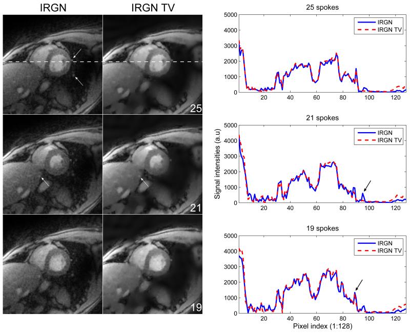
Reconstructions of real-time images of the beating heart are displayed in Fig. 6 together with plots of the signal intensities across an indicated horizontal line. Results for 25 (R ≈ 8.0), 21 (R ≈ 9.6), and 19 (R ≈ 10.6) acquired spokes are shown, corresponding to image acquisition times of 50ms, 41ms, and 38ms. For all reconstructions, βmin = 5 · 10−3 was used. The image reconstructed from the 25 spokes data set does not show streaking artifacts for both IRGN and IRGN-TV. However, noise amplification is much stronger for IRGN. In contrast, reconstructions from 21 and 19 spokes show residual streaking artifacts due to increased subsampling, which are again reduced in the images reconstructed with IRGN-TV.
Figure 6.
Comparison of IRGN (left) and IRGN-TV (middle) for radial sampling of a human heart (βmin = 5·10−3). Top: 25 spokes. Highlighted are structures with little signal intensity that can be lost due to strong TV regularization. Middle: 21 spokes. Highlighted are structures of similar size but slightly higher signal intensity that are preserved even in case of TV regularization. Bottom: 19 spokes. The plots on the right show signal intensities across a horizontal line, indicated in the top row of the reconstruction results. The ability of IRGN-TV to preserve sharp edges is highlighted in the plot of the reconstruction from 19 spokes. The arrow marks the sharp boarder of the ventricle, which is depicted equally well with IRGN and IRGN-TV. The undesired loss of a small structure is highlighted in the plot of the reconstruction from 21 spokes. The plot crosses two adjacent vessels, which are both represented in the IRGN solution, but only the left one appears in the IRGN-TV reconstruction.
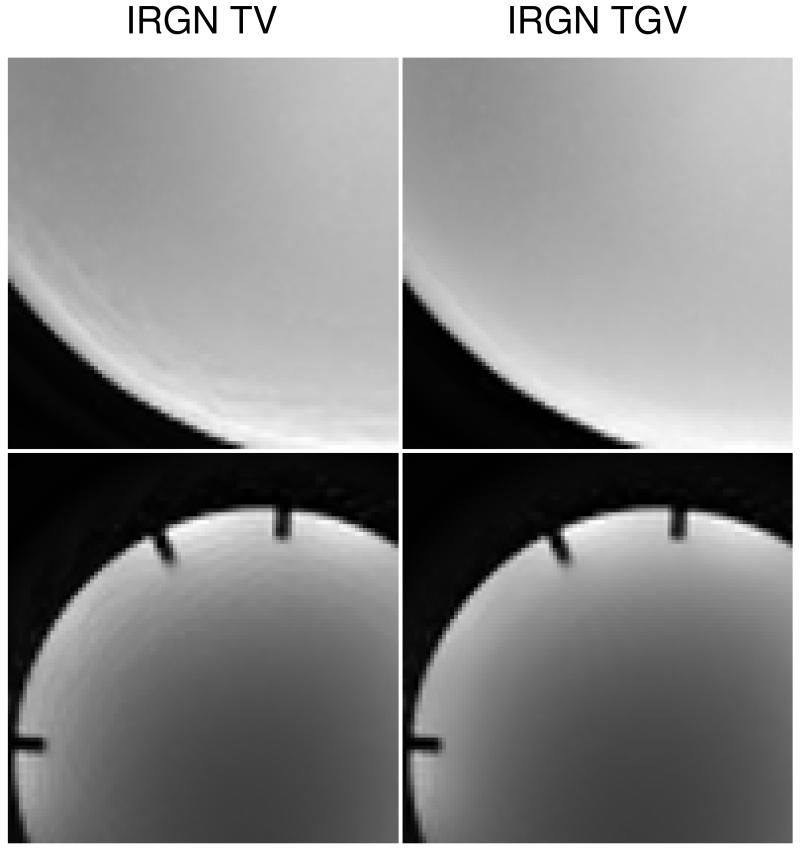
The effect of TGV regularization is demonstrated in Fig. 7. It shows highlighted regions of both phantom images affected by staircasing artifacts (pseudorandom and radial sampling, see Figs. 1 and 5) using TV as well as TGV regularization, both with βmin = 5 · 10−3. The staircasing artifact is completely removed in the reconstruction with the IRGN-TGV method.
Figure 7.
Comparison of IRGN-TV and IRGN-TGV for phantom data (top: pseudorandom sampling; bottom: radial sampling; both: βmin = 5 · 10−3). Left: IRGN-TV (magnified details from Figs. 1, R = 10 and 5). Modulations from the coil sensitivities lead to pronounced staircasing artifacts from TV regularization. Right: IRGN-TGV. Staircasing artifacts are completely removed for TGV regularization.
DISCUSSION
The results from this work demonstrate that pronounced improvements in reconstruction quality of parallel imaging with nonlinear inversion can be achieved with TV and TGV based regularization instead of a simple L2 penalty. If moderate acceleration is used (e.g. Fig. 1, case of R = 4), TV serves as a stabilization term against noise amplification, which otherwise limits the practical use of parallel imaging to low acceleration factors. In cases where acceleration is pushed to its limits (Fig. 1, case of R = 10; Figs. 5 and 6), TV also leads to an additional removal of undersampling artifacts when combined with trajectories that produce incoherent aliasing. However, it must be noted that in this case, small image features with low contrast may also be removed during the reconstruction. This effect can be observed for some smaller structures, which are highlighted in Fig. 6. It can be seen in the top row that structures with low signal, which are still visible in conventional IRGN reconstructions, are removed when TV is applied. However, as indicated by the highlights in the middle row, objects with a slightly higher signal intensity, even though of same size, are preserved in both reconstructions. These effects are also represented in the cross-sectional plots. The elimination of structures like noise or residual streaking artifacts is visible as a reduced amount of high frequency oscillations in the IRGN-TV plots. Note that due to the nature of TV, blurring of sharp edges does not occur. This can be observed, e.g., at the sharp border of the ventricle, which is preserved equally well with IRGN and IRGN-TV.
As can be seen from Fig. 4, the results of IRGN-TV are comparable to those achievable by TV filtering, since the regularization term is the same in both cases. However, this requires (manual) parameter tuning in the case of TV filtering, even though the data sets were very similar in terms of anatomy, sampling pattern and normalization. In contrast, IRGN-TV performed similarly well on both data sets for the same choice of parameters, which can be attributed to the fact that the data fitting term in IRGN-TV considers only the actually acquired k-space coefficients. This allows more accurate discrimination between image content and reconstruction artifacts. On the other hand, the data fitting term in TV filtering is based solely on image-space contrast. Furthermore, due to the iterative nature of the IRGN method, the noise suppression properties of strong TV regularization can take effect even for a small final regularization parameter value.
Our Matlab implementations reconstructed a single slice in a few minutes, where IRGN-TV took roughly 10% more time than IRGN (and similarly, IRGN-TGV was about 10% slower than IRGN-TV). It is possible to exploit the differentiability of the data consistency term to apply more efficient minimization algorithms such as the method of conjugate gradients in the case of IRGN or order optimal convex minimization methods such as those investigated in (33) for IRGN-TV and IRGN-TGV. Because this work focused on the effect of the different regularization techniques on image quality, the same primal-dual extra-gradient method was used as inner algorithm in all cases to allow a direct comparison for identical parameter choices. In this context, it should be noted that the parameters for the iteratively regularized Gauss–Newton method were independent of the chosen regularization term, and only depended on the trajectory type. Similarly, since the norm of the forward operator is estimated in the algorithm, the fixed parameters for the primal-dual extra-gradient methods were independent of the data set.
In this work, the flexibility to include different regularization terms was demonstrated on 2D examples, where each image (slice, i.e., 2D partition of a 3D data set, or frame of a time series) was reconstructed individually. While computationally more demanding, the extension of the penalties into a third space or a time dimension should further improve the image quality due to temporal redundancies in dynamic sequences – an effect that is well described in the literature (41-44). For example, earlier work has shown that residual streaking artifacts in radial imaging can be removed with the use of a median filter in the time dimension when using an interleaved k-space sampling scheme (45). Since the median filter can be interpreted as solving an L1 minimization problem, it is expected that the inclusion of a corresponding penalty – either in the form of an L1 penalty on the difference between the current and previous slice or frame, or of a higher-dimensional T(G)V penalty on the full data set – will yield even better results. The resulting convex minimization problems can be solved using the same primal-dual extra-gradient method as employed in this work.
Another possible extension of this work is the integration of additional information about the physical signal model into the functional in Eq. 2. An important application is mapping of relaxation parameters in multi echo sequences (46, 47). Here, the framework of nonlinear inverse problems makes it straightforward to perform parameter identification during the reconstruction. Since the parameters are thus estimated directly from the raw data, instead of from reconstructed images, better quantification is possible.
CONCLUSIONS
This work describes an approach to include additional variational penalties in parallel imaging with nonlinear inversion. The presented algorithms combine the advantages of nonlinear inversion, i.e., improved image quality through a better estimation of the coil sensitivities, with the advantageous properties of TV-based regularization terms. In addition to reducing the noise, the regularization is able to remove undersampling artifacts when combined with sampling strategies that produce incoherent aliasing, such as radial and pseudorandom sampling. The approach has the additional benefit that the inclusion of physiological parameters, either as additional penalties or as unknown parameters to be reconstructed, is straightforward.
Acknowledgments
Grant sponsor: Austrian Science Fund: Grant number SFB F3209-18.
REFERENCES
- 1.Bauer F, Kannengiesser S. An alternative approach to the image reconstruction for parallel data acquisition in MRI. Math Meth Appl Sci. 2007;30:1437–1451. [Google Scholar]
- 2.Ying L, Sheng J. Joint image reconstruction and sensitivity estimation in SENSE (JSENSE) Magn Reson Med. 2007;57(6):1196–1202. doi: 10.1002/mrm.21245. [DOI] [PubMed] [Google Scholar]
- 3.Uecker M, Hohage T, Block KT, Frahm J. Image reconstruction by regularized nonlinear inversion – joint estimation of coil sensitivities and image content. Magn Reson Med. 2008;60(3):674–682. doi: 10.1002/mrm.21691. [DOI] [PubMed] [Google Scholar]
- 4.Uecker M, Karaus A, Frahm J. Inverse reconstruction method for segmented multishot diffusion-weighted MRI with multiple coils. Magn Reson Med. 2009;62(5):1342–1348. doi: 10.1002/mrm.22126. [DOI] [PubMed] [Google Scholar]
- 5.Sodickson DK, Manning WJ. Simultaneous acquisition of spatial harmonics (SMASH): fast imaging with radiofrequency coil arrays. Magn Reson Med. 1997;38(4):591–603. doi: 10.1002/mrm.1910380414. [DOI] [PubMed] [Google Scholar]
- 6.Pruessmann KP, Weiger M, Scheidegger MB, Boesiger P. SENSE: sensitivity encoding for fast MRI. Magn Reson Med. 1999;42(5):952–962. [PubMed] [Google Scholar]
- 7.Griswold MA, Jakob PM, Heidemann RM, Nittka M, Jellus V, Wang J, Kiefer B, Haase A. Generalized autocalibrating partially parallel acquisitions (GRAPPA) Magn Reson Med. 2002;47(6):1202–1210. doi: 10.1002/mrm.10171. [DOI] [PubMed] [Google Scholar]
- 8.Knoll F, Clason C, Uecker M, Stollberger R. Improved reconstruction in non-cartesian parallel imaging by regularized nonlinear inversion; Proceedings of the 17th Scientific Meeting and Exhibition of ISMRM; Honolulu, HI. 2009. [Google Scholar]
- 9.Uecker M, Zhang S, Frahm J. Nonlinear inverse reconstruction for real-time MRI of the human heart using undersampled radial FLASH. Magn Reson Med. 2010;63(6):1456–1462. doi: 10.1002/mrm.22453. [DOI] [PubMed] [Google Scholar]
- 10.Chang T, He L, Fang T. MR image reconstruction from sparse radial samples using Bregman iteration; Proceedings of the 14th Scientific Meeting and Exhibition of ISMRM; Seattle. 2006.p. 696. [Google Scholar]
- 11.Block KT, Uecker M, Frahm J. Undersampled radial MRI with multiple coils. Iterative image reconstruction using a total variation constraint. Magn Reson Med. 2007;57(6):1086–1098. doi: 10.1002/mrm.21236. [DOI] [PubMed] [Google Scholar]
- 12.Liu B, King K, Steckner M, Xie J, Sheng J, Ying L. Regularized sensitivity encoding (SENSE) reconstruction using Bregman iterations. Magn Reson Med. 2009;61(1):145–152. doi: 10.1002/mrm.21799. [DOI] [PubMed] [Google Scholar]
- 13.Candes EJ, Romberg J, Tao T. Robust uncertainty principles: exact signal reconstruction from highly incomplete frequency information. IEEE Transactions on Information Theory. 2006;52(2):489–509. [Google Scholar]
- 14.Donoho DL. Compressed sensing. IEEE Transactions on Information Theory. 2006;52(4):1289–1306. [Google Scholar]
- 15.Lustig M, Lee J, Donoho D, Pauly J. Faster imaging with randomly perturbed, under-sampled spirals and L1 reconstruction; Proceedings of the 13h Scientific Meeting and Exhibition of ISMRM; Miami Beach, FL. 2005.p. 685. [Google Scholar]
- 16.Lustig M, Donoho D, Pauly JM. Sparse MRI: The application of compressed sensing for rapid MR imaging. Magn Reson Med. 2007;58(6):1182–1195. doi: 10.1002/mrm.21391. [DOI] [PubMed] [Google Scholar]
- 17.Gamper U, Boesiger P, Kozerke S. Compressed sensing in dynamic MRI. Magnetic Resonance in Medicine. 2008;59(2):365–373. doi: 10.1002/mrm.21477. [DOI] [PubMed] [Google Scholar]
- 18.Xiang QS. Accelerating MRI by skipped phase encoding and edge deghosting (SPEED) Magn Reson Med. 2005;54(5):1112–1117. doi: 10.1002/mrm.20453. [DOI] [PubMed] [Google Scholar]
- 19.Lustig M, Pauly JM. Calibrationless parallel imaging reconstruction by structured low-rank matrix completion; Proc. Intl. Soc. Mag. Reson. Med.; 2010; p. 2870. [DOI] [PMC free article] [PubMed] [Google Scholar]
- 20.Rudin LI, Osher S, Fatemi E. Nonlinear total variation based noise removal algorithms. Phys D. 1992;60(1-4):259–268. [Google Scholar]
- 21.Liang Z, Bammer R, Ji J, Pelc N, Glover G. Making better SENSE: wavelet denoising, Tikhonov regularization, and total least squares; Proceedings of the 10th Scientific Meeting and Exhibition of ISMRM; Honolulu, HI. 2002.p. 2388. [Google Scholar]
- 22.Lin FH, Kwong KK, Belliveau JW, Wald LL. Parallel imaging reconstruction using automatic regularization. Magn Reson Med. 2004;51(3):559–567. doi: 10.1002/mrm.10718. [DOI] [PubMed] [Google Scholar]
- 23.Hoge WS, Brooks DH, Madore B, Kyriakos W. On the regularization of SENSE and space-RIP in parallel MR imaging; Proc. IEEE Int Biomedical Imaging: Nano to Macro Symp.; 2004.pp. 241–244. [Google Scholar]
- 24.Hoge WS, Brooks DH, Madore B, Kyriakos WE. A tour of accelerated parallel MR imaging from a linear systems perspective. Concepts in Magnetic Resonance Part A. 2005;27A:17–37. [Google Scholar]
- 25.Bredies K, Kunisch K, Pock T. Total generalized variation. SIAM Journal on Imaging Sciences. 2010;3(3):492–526. [Google Scholar]
- 26.Knoll F, Bredies K, Pock T, Stollberger R. Second order total generalized variation (TGV) for MRI. Magn Reson Med. 2010;65(2):480–491. doi: 10.1002/mrm.22595. [DOI] [PMC free article] [PubMed] [Google Scholar]
- 27.Lustig M, Pauly JM. SPIRiT: Iterative self-consistent parallel imaging reconstruction from arbitrary k-space. Magn Reson Med. 2010;64(2):457–471. doi: 10.1002/mrm.22428. [DOI] [PMC free article] [PubMed] [Google Scholar]
- 28.Bakushinsky AB, Kokurin MY. Iterative methods for approximate solution of inverse problems. Vol. 577. Springer; Dordrecht: 2004. (Mathematics and its Applications). [Google Scholar]
- 29.Engl HW, Hanke M, Neubauer A. Regularization of inverse problems. Vol. 375. Kluwer Academic Publishers Group; Dordrecht: 1996. (Mathematics and its Applications). [Google Scholar]
- 30.Blaschke B, Neubauer A, Scherzer O. On convergence rates for the iteratively regularized Gauss-Newton method. IMA J Numer Anal. 1997;17(3):421–436. [Google Scholar]
- 31.Hohage T. Logarithmic convergence rates of the iteratively regularized Gauss-Newton method for an inverse potential and an inverse scattering problem. Inverse Problems. 1997;13(5):1279–1299. [Google Scholar]
- 32.Pock T, Cremers D, Bischof H, Chambolle A. An algorithm for minimizing the Mumford-Shah functional; International Conference on Computer Vision (ICCV); 2009.pp. 1133–1140. [Google Scholar]
- 33.Chambolle A, Pock T. A first-order primal-dual algorithm for convex problems with applications to imaging. J Math Imaging Vis. 2011;40:120–145. [Google Scholar]
- 34.Buehrer M, Pruessmann KP, Boesiger P, Kozerke S. Array compression for MRI with large coil arrays. Magn Reson Med. 2007;57(6):1131–1139. doi: 10.1002/mrm.21237. [DOI] [PubMed] [Google Scholar]
- 35.Knoll F, Clason C, Diwoky C, Stollberger R. Adapted random sampling patterns for accelerated MRI. Magn Reson Mater Phy (MAGMA) 2011;24(1):43–50. doi: 10.1007/s10334-010-0234-7. [DOI] [PMC free article] [PubMed] [Google Scholar]
- 36.Frahm J, Haase A, Matthaei D. Rapid NMR imaging of dynamic processes using the FLASH technique. Magn Reson Med. 1986;3(2):321–327. doi: 10.1002/mrm.1910030217. [DOI] [PubMed] [Google Scholar]
- 37.Riederer SJ, Tasciyan T, Farzaneh F, Lee JN, Wright RC, Herfkens RJ. MR fluoroscopy: technical feasibility. Magn Reson Med. 1988;8(1):1–15. doi: 10.1002/mrm.1910080102. [DOI] [PubMed] [Google Scholar]
- 38.Wright RC, Riederer SJ, Farzaneh F, Rossman PJ, Liu Y. Real-time MR fluoroscopic data acquisition and image reconstruction. Magn Reson Med. 1989;12(3):407–415. doi: 10.1002/mrm.1910120314. [DOI] [PubMed] [Google Scholar]
- 39.Zhang S, Block KT, Frahm J. Magnetic resonance imaging in real time: advances using radial FLASH. J Magn Reson Imaging. 2010;31(1):101–109. doi: 10.1002/jmri.21987. [DOI] [PubMed] [Google Scholar]
- 40.Fessler JA, Sutton BP. Nonuniform fast Fourier transforms using min-max interpolation. IEEE Transactions on Signal Processing. 2003;51(2):560–574. [Google Scholar]
- 41.Madore B, Glover GH, Pelc NJ. Unaliasing by fourier-encoding the overlaps using the temporal dimension (UNFOLD), applied to cardiac imaging and fMRI. Magn Reson Med. 1999;42(5):813–828. doi: 10.1002/(sici)1522-2594(199911)42:5<813::aid-mrm1>3.0.co;2-s. [DOI] [PubMed] [Google Scholar]
- 42.Kellman P, Epstein FH, McVeigh ER. Adaptive sensitivity encoding incorporating temporal filtering (TSENSE) Magn Reson Med. 2001;45(5):846–852. doi: 10.1002/mrm.1113. [DOI] [PubMed] [Google Scholar]
- 43.Tsao J, Boesiger P, Pruessmann KP. k-t BLAST and k-t SENSE: dynamic MRI with high frame rate exploiting spatiotemporal correlations. Magn Reson Med. 2003;50(5):1031–1042. doi: 10.1002/mrm.10611. [DOI] [PubMed] [Google Scholar]
- 44.Xu D, King KF, Liang ZP. Improving k-t SENSE by adaptive regularization. Magn Reson Med. 2007;57(5):918–930. doi: 10.1002/mrm.21203. [DOI] [PubMed] [Google Scholar]
- 45.Uecker M, Zhang S, Voit D, Karaus A, Merboldt KD, Frahm J. Real-time MRI at a resolution of 20 ms. NMR Biomed. 2010;23:986–994. doi: 10.1002/nbm.1585. [DOI] [PubMed] [Google Scholar]
- 46.Block KT, Uecker M, Frahm J. Model-based iterative reconstruction for radial fast spin-echo MRI. IEEE Trans Med Imaging. 2009;28(11):1759–1769. doi: 10.1109/TMI.2009.2023119. [DOI] [PubMed] [Google Scholar]
- 47.Doneva M, Boernert P, Eggers H, Stehning C, Senegas J, Mertins A. Compressed sensing reconstruction for magnetic resonance parameter mapping. Magn Reson Med. 2010;64(4):1114–1120. doi: 10.1002/mrm.22483. [DOI] [PubMed] [Google Scholar]


