Semantic and acoustic analysis of speech by functional networks with distinct time scales

Abstract

Speech perception requires the successful interpretation of both phonetic and syllabic information in the auditory signal. It has been suggested by Poeppel (2003) that phonetic processing requires an optimal time scale of 25 ms while the time scale of syllabic processing is much slower (150–250ms). To better understand the operation of brain networks at these characteristic time scales during speech perception, we studied the spatial and dynamic properties of EEG responses to five different stimuli: (1) amplitude modulated (AM) speech, (2) AM speech with added broadband noise, (3) AM reversed speech, (4) AM broadband noise, and (5) AM pure tone. Amplitude modulation at gamma band frequencies (40 Hz) elicited steady-state auditory evoked responses (SSAERs) bilaterally over primary auditory cortices. Reduced SSAERs were observed over the left auditory cortex only for stimuli containing speech. In addition, we found over the left hemisphere, anterior to primary auditory cortex, a network whose instantaneous frequencies in the theta to alpha band (4–16 Hz) are correlated with the amplitude envelope of the speech signal. This correlation was not observed for reversed speech. The presence of speech in the sound input activates a 4–16 Hz envelope tracking network and suppresses the 40-Hz gamma band network which generates the steady-state responses over the left auditory cortex. We believe these findings to be consistent with the idea that processing of the speech signals involves preferentially processing at syllabic time scales rather than phonetic time scales.

1. Introduction

Human beings possess an amazing ability to recognize speech in complex acoustic scenes. We can track one person’s speech out of an amalgamation of conversations in a clamorous environment (Cherry, 1953). Bregman (1990) has proposed a theoretical framework for Auditory Scene Analysis (ASA) that divides the processing of speech input into two stages. The earlier stage, called primitive segregation, parses the acoustic input to provide perceptual cues. The next stage, called schema-based segregation, sets up the auditory scene with distinct cognitive objects reconstructed from the cues. In this model, during the acoustical analysis, speech and non-speech stimuli share similar neural processes, but once the incoming stimuli are recognized as speech, more extensive cortical processing can take place. Previous studies have identified the functional neuroanatomy of language including cortical areas specifically related to acoustic analysis during speech processing using PET and fMRI (Hickok and Poeppel, 2004; Reyes et al., 2004; Meyer et al., 2005; Benson et al., 2006). The organization of these areas into functional networks that process incoming speech signals may depend critically on temporal properties of speech.

In general, speech signals contain more than one time-scale of perceptual organization which may be parsed by distinct brain networks. For instance, networks processing phonemes are believed to operate on an optimal time scale of around 25 ms, in order to best encode the formant transitions in stop consonants (Poeppel, 2003). Speech signals also contain information at slower time scales, and specific cortical networks may be activated by information at corresponding time scales to facilitate language processing. In contrast to the rapid time scale of phonemic processing, syllabic parsing may involve networks that operate at a slower characteristic time scale of 150–250 ms (Luo and Poeppel, 2007). The phonemic (~25 ms) and syllabic (15–250 ms) time scales correspond respectively to the periods of gamma (40 Hz) and theta (4–7 Hz) oscillations observed in human EEG or MEG recordings.

Gamma band oscillations have been recorded from auditory cortex in humans using EEG (Picton et al., 2003) or MEG (Galambos et al., 1981) and in animal models (Markessis et al., 2006) using a variety of stimuli including simple tones, noise bursts, and speech. Previous studies have suggested that stronger gamma oscillations are evoked over the left auditory cortex by the onset of syllables than noise (Palva et al., 2002), suggesting speech processing networks operating at gamma band frequencies. However, the contribution of these gamma band responses to speech processing are difficult to investigate in conventional evoked potential experiments because of their low signal-to-noise (SNR) ratio and susceptibility to EMG artifacts (Nunez and Srinivasan, 2006; Fatourechi et al., 2007). In most previous studies, gamma-band auditory responses have mostly been recorded by averaging many repetitions of brief tone or noise bursts or in response to isolated syllables.

Steady-State Auditory Evoked Responses (SSAERs) are elicited by periodic amplitude modulation of auditory stimuli which evokes an oscillatory response at the modulation frequency (and harmonics). In humans, the SSAER is commonly observed in the gamma band with peak response at around 40 Hz (Rickards and Clark, 1982). SSAERs offer the advantage of higher signal-to-noise ratio (SNR) than other evoked potential methods to detect gamma band responses to auditory stimuli. Most of previous SSAER studies have used low-level auditory stimuli such as pure tones or noise to evaluate the functionality of the auditory system in early hearing loss detection or to measure the cortical response to these simple stimuli in cognitive studies (Wienbruch et al., 2006; Picton et al., 2007; Schadow et al., 2007). To our knowledge, no previous studies have investigated the properties of SSAERs evoked by speech. In this study, we contrast the activity of gamma band networks by using SSAERs evoked by both speech and non-speech stimuli. Our analysis focuses on the hemispheric specificity of differences observed between the SSAER evoked these stimuli.

Previous studies have suggested possible operational properties of theta (and alpha) oscillations in speech processing. Ahissar and colleagues (2001) manipulated the frequency content of speech temporal envelope and found that successful speech comprehension depends on the matching between the frequency capacity of auditory cortex neurons (below 16 Hz, theta to alpha band) and the spectral focus of the speech envelope. Luo and Poeppel (2007) found that theta band phase coherence between MEG and the envelope of the speech stimulus is correlated with speech intelligibility. They believed that this correlation indicates the syllabic level processing of speech at the characteristic time scale of 150–250 ms (corresponding to 4–7 Hz). To investigate the relationship between EEG signals and the envelope of the speech stimulus, we first applied the Hilbert–Huang Transformation (HHT) to decompose the EEG signals into intrinsic components with smooth envelopes (Huang and Shen, 2005). We evaluated the time course of the amplitude and frequency of theta and alpha band components to determine whether they are correlated with the amplitude envelope of the speech stimuli.

The present study seeks to investigate cortical processing of speech and non-speech stimuli by simultaneously investigating gamma band cortical responses at “phonetic” time scales and theta/alpha band responses at “syllabic” time scales in a unified paradigm. The set of stimuli we investigated consists of speech, speech in noise, reversed speech, noise, and pure tones. We demonstrate reduced gamma band SSAER over the left hemisphere specifically for speech. Instead, instantaneous frequencies of theta/alpha components of EEG signals recorded in the left hemisphere are correlated with the amplitude envelope of the speech. Our results further substantiate the idea that speech signals are preferentially processed at syllabic time scales in the theta/alpha band and moreover demonstrate reduced processing at phonetic time scales in the gamma band.

2. Results

We evaluated the SSAER signal-to-noise ratio (SNR) for each of the five stimulus conditions (pure tones, noise, speech, speech in noise, and reversed speech). For the speech and reversed speech data, the correlation between the speech envelope and the Hilbert–Huang Transform (HHT) of the EEG signals was further analyzed. We employed a bootstrapping procedure for statistical tests. The details of these procedures are presented in Section 4.

2.1. SSAER power analysis shows decreased responses over the left for speech conditions

The SSAER was detected in every stimulation condition in every subject, at the frequency matching the exact frequency of the amplitude modulation. Fig. 1 shows the power spectrum and SNR spectrum from a single trial in one subject. The plots on the left column show the entire spectrum, and the plot on the right column are zoomed in on the SSAER frequency. SNR was calculated by normalizing the power at each frequency f to the average power in the 2 Hz wide band surrounding f. The SSAER is clearly visible in the SNR spectrum, which normalizes the signals for variation in individual subject’s EEG amplitudes and removes high-amplitude broadband signals that overlap the SSAER frequency, e.g., EMG artifacts.

Fig. 1.

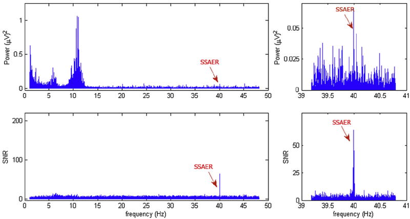
the Power spectrum and SNR spectrum of one EEG segment. Top row: the full spectrum and a zoom-in view. The 40-Hz SSAER is distinguishable from the surrounding components. Bottom row: SNR spectrum. The 40-Hz SSAER is the only significant component throughout the entire spectrum, and the peaks in the surrounding bins are suppressed.

The trial and subject averaged SSAER power spectrum for both the left and right ROIs for each type of stimuli are shown in Fig. 2. The steady-state responses, marked in red, are clearly visible in all conditions expect in the left ROI of AM speech and AM speech plus noise conditions, where the responses are below the SNR significance threshold of 5.14 (with the values being 2.58 and 2.80, respectively). However, in the right ROIs for these two conditions, the responses are much larger and significant. Among the total of 72 (9 subjects, 8 trials each) EEG recordings in the AM speech condition, 59 recordings (81.9%) had larger SSAER power over the right than that over the left. For the AM speech plus background noise condition, 57 out of the 72 recordings (83.3%) showed this pattern of difference in SSAER power. In contrast, for the AM pure tone condition, only 27 out of the 72 recordings have larger right responses (37.5%). And similarly, for AM white noise condition, 28 out 72 showed larger right responses (38.9%); for AM reversed speech condition, this pattern is detected in 39 out of 72 recordings (54.2%).

Fig. 2.

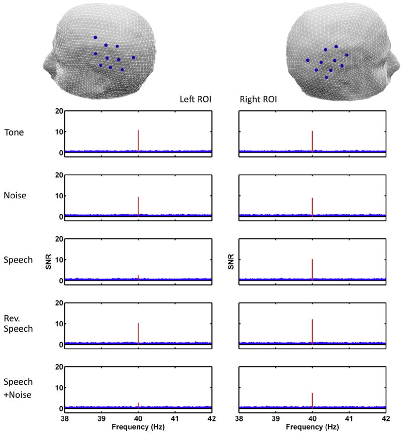
Zoomed in views of average SNR spectra over the left and right ROI by experimental conditions. Ten channels from the temporal–parietal area of each hemisphere were selected to generate these plots, as indicated in the head models in the first row. The red bin at the center of each plot designates the 40-Hz SSAER power in SNR units. SNR is calculated as the ratio of the power at the peak to the average power in a 2-Hz band (80 bins) surrounding it. Each plot is generated by averaging the log₁₀ (SNR) across the selected 10 channels for all trials and all subjects, then converting the value back to linear scale.

Fig. 3 shows the topographic maps of SSAER for all five experimental conditions averaged across subjects. Responses are distributed mainly along the temporal–parietal regions of both hemispheres but extended to the frontal and occipital regions in some subjects. This pattern of response is consistent with the findings of other SSAER studies (e.g., Picton et al., 2003). For AM tone, noise, and reverse speech conditions, significant responses could be seen on both left and right hemisphere, while for AM speech and speech plus background noise conditions, the responses on the left side are much weaker.

Fig. 3.

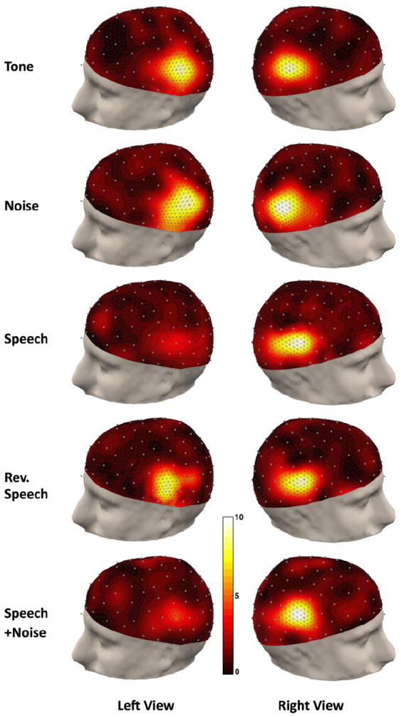
Topographic display of the SSAER SNR distributions averaged across subjects. For each experiment condition the data are averaged across all available trials, and the left and right views are presented with focuses on the temporal–parietal areas. All distributions are plotted on the same color scale.

Statistical comparisons of the SNR for each ROI between each experimental condition and the omnibus mean are shown in the left column of Fig. 4. Over the left hemisphere, the response for AM speech and AM speech plus noise conditions are significantly lower than the omnibus mean at a 0.05 alpha-level. The higher response for AM pure tone condition is marginally significant with a p-value of 0.0494. Over the right hemisphere, none of the responses of five conditions is significantly different than the omnibus mean. A pairwise comparison of the mean response over each ROIs between all conditions is summarized in Table 1. Since a total of 10 comparisons were made for each group of data, an adjusted alpha-level of 0.001 was used as the significance threshold. At this level, we found that over the left hemisphere, all contrasts between speech or speech plus background noise and the other conditions were highly significant. Meanwhile, comparisons that do not involve speech or speech plus noise were all not significant. No significant difference between the SSAER responses of these two conditions were found, and both stimuli produced the same lateralization effects of SSAER distribution. Over the right hemisphere, we found no significant difference.

Fig. 4.

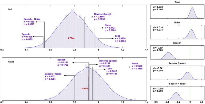
Comparisons of mean SSAER power. Left column: comparisons against the omnibus mean. The omnibus mean is the grand average of SSAER power across all data. x-Axes are in unit of log 10(SNR). The estimated probability densities of the omnibus mean for left and right ROIs were generated separately, each from 20,000 bootstrap resampling repetitions. The mean values of the densities are in red digits. The location and values of the observed mean SSAER power of each condition are marked in purple. The corresponding p-values, defined as the number of samples distributed to the tail of the estimated density function of the omnibus mean, are also given. Right column: comparison between left and right ROIs. The random variable d is formulated as the mean SSAER difference of left and right ROIs, subtracting the mean SSAER difference of two arbitrarily generated groups randomly sampled from the pooled data (see method for details). The unit of x-axes is log 10(SNR). For each particular condition, 10,000 bootstrap resamplings of the 48 trails were performed to generate the distribution. The estimated probability density functions of d were computed using a kernel-smoothing method. The mean location of each distribution, as well as the p-value of getting an observation more extreme than 0, are shown on the upper right corner for each plot.

Table 1.

Result of the pairwise comparisons of all experimental conditions of the mean SSAER power in both ROIs. The value in each cell is the probability of observing the measured difference between that pair, given that the null hypothesis of no difference between the pair. Estimated population density of each variable to be tested was obtained via 10,000 bootstrap procedures, as described in the method section. Since there is a total of 10 comparisons of the ROI for each side, a Bonferroni corrected significance level of 0.001 was used. Significant differences are identified with bold fonts.

Left	Tone	Noise	Speech	Rev. Speech	Right	Tone	Noise	Speech	Rev. Speech
Noise	0.3426	–	–	–	Noise	0.4856	–	–	–
Speech	0.0000	0.0000	–	–	Speech	0.2332	0.2213	–	–
Rev. Speech	0.0321	0.0482	0.0001	–	Rev. Speech	0.2680	0.2816	0.4858	–
Speech+Noise	0.0000	0.0001	0.3116	0.0002	Speech+Noise	0.0040	0.0024	0.0096	0.0177

The results of comparisons of the mean SSAER power difference between hemispheres (Fig. 4, right column) within each condition revealed significant differences in the AM speech and AM speech plus background noise conditions, both with p-value below 0.001. This confirmed the decreased SSAER power over left ROI for these conditions. For the remaining three experimental conditions, the null hypothesis that the SSAER power over the left and right ROIs are the same could not be rejected.

2.2. Correlation analysis reveals matching between EEG components and the envelopes of speech

Inspired by the notion (Ahisar et al., 2001; Luo and Poeppel, 2007) that theta or alpha band cortical activity follows the temporal envelope of the stimulus during speech perception, we explored the correlation between the temporal envelope of the speech stimuli, low-pass filtered below 30 Hz, and EEG signals decomposed using a Hilbert–Huang Transform into intrinsic mode functions (IMFs). The plots on panel A of Fig. 5 show 5 s of raw EEG and all of the IMFs. The IMFs are defined by statistical properties of the envelope of the signals. They may be considered roughly as outputs of a set of band limited filters with the choices of bandwidths adapted to the intrinsic modes of the original signal. This can be seen clearly in part C and D of Fig. 5 which shows the power spectrum of the 5 s of EEG and each of the IMFs. For this 5-s epoch, there are 3 IMFs (labeled here 5, 6, and 7) with power in the theta and alpha bands.

Fig. 5.

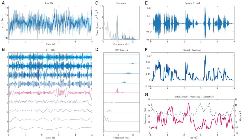
An example of the HHT result and instantaneous frequency of certain HHT component follows the speech envelope. Panel A: the original EEG recording during listening to speech stimulus. No preprocessing was performed on the EEG data except than removing the linear trend. B: the IMFs from an EMD of the EEG signal. The fifth component in red, which contains mostly theta-alpha band energy, is the one used to calculate the instantaneous frequency in panel G. C: the power spectrum of the original EEG. The x-axis is in logarithmic scale. D: the power spectra of the corresponding IMF components in panel B. The x-axis is also in log scale. E: waveform of the original speech stimulus. F: the temporal envelope of the speech waveform. G: the instantaneous frequency and instantaneous amplitude of the selected (5th) IMF. This component has spectra content mainly focuses on alpha-theta band. The instantaneous frequency is shown in red solid line, and the instantaneous amplitude in blue dashed line. The correlation coefficient between the instantaneous frequency and the speech envelope is 0.3014, and the correlation coefficient between the instantaneous amplitude and the speech envelope is −0.1042.

The upper and lower envelopes of each IMF are approximately symmetric about zero. This property ensures that IMFs have well-behaved envelopes, and that instantaneous amplitude and instantaneous frequency (rate of phase change) can be calculated using a Hilbert Transform. In part E and F of Fig. 5 the waveform of the speech stimulus and its low pass filtered envelope (30 Hz cutoff) are shown. Part G of Fig. 5 shows the instantaneous amplitude and instantaneous frequency of IMF 5. The instantaneous frequency apparently tracks the envelope of the speech signal—as the amplitude of the speech increases, the frequency of the oscillation increases.

We tested the correlation between the speech envelope and amplitude and instantaneous frequencies of each IMF obtained at each channel. We found no evidence of tracking of the amplitude of the speech by the amplitude envelope of any of the IMFs. Correlation with the speech envelope (ccSpeech) could be observed only for the instantaneous frequencies of the IMFs with power in the theta and alpha band. We computed the correlations for two more conditions: ccControl, which is defined as the correlation between the same set of IMF instantaneous frequencies and envelopes from random mismatching speech clips unheard by the subject; and ccReverse, which is the correlation between the IFs from the reversed speech EEG data and the corresponding (reversed) stimuli envelope. The empirical distribution for each condition was obtained using 10,000 bootstrap samples across all available subjects, trials, and channels. The result is summarized in Fig. 6a. The density curves suggest significant correlation for ccSpeech. (H0: mean (ccSpeech) ⩵ 0, p<0.001; H0: mean(ccSpeech) ⩵ mean(ccControl), p<0.001) Furthermore, significant ccSpeech correlation was found in all nine subjects. In contrast, this pattern is not observed for ccControl and ccRevSpeech conditions. The mean values of ccControl and ccRevSpeech are not significantly different.

Fig. 6.

The empirical distribution of EEG correlation with speech stimuli, reverse speech stimuli, and with control signal and the topographic distribution of the correlation coefficients. The empirical distributions were calculated from the median of 10,000 bootstrap samples of all trials, subjects and channels. The topographic distribution of estimated correlation for ccSpeech is calculated from the same bootstrap resampling procedure.

The topographic distribution of estimated correlation for ccSpeech, averaged across all subjects and trials, is plotted in Fig. 6b. ccSpeech is highest over the left hemisphere and presumably over auditory cortex. However, compared with the topography of SSAER (see Fig. 3), the electrodes showing the highest correlation are generally shifted toward more central and anterior regions. Selecting 10 electrodes based on this topography, we calculated the descriptive statistics (The 5th, 50th and 95th percentile of instantaneous frequencies.) of the component of highest correlation with stimuli envelope (see Table 2) within this region for each subject to provide better understanding of the spectral properties of the speech-envelope-correlated signal. Correlations of small to medium size are observed in all subjects and the components mostly fluctuate around the theta and alpha bands.

Table 2.

Components of maximum correlation with speech envelope within 10 selected channels for all subjects. The 5th, 50th and 95th percentiles of frequency distribution of these components are also presented.

Subject	Max ccSpeech	Median IF (Hz)	IF: 5th Percentile (Hz)	IF: 95th percentile (Hz)
1	0.2423	7.37	4.22	13.35
2	0.2198	13.59	8.31	25.37
3	0.2214	10.32	4.43	15.02
4	0.2569	10.28	5.51	15.44
5	0.2494	13.01	5.35	24.65
6	0.3874	11.52	4.91	18.74
7	0.3486	7.23	3.18	14.26
8	0.2444	7.33	3.74	14.14
9	0.2237	16.82	8.27	29.11

3. Discussion

In general, speech signals contain more than one temporal scale of perceptual organization. During successful speech perception, various brain networks operate on these different levels of information. Phonemic processing networks are believed to operate on an optimal time scale of around 25 ms, in order to best encode the formant transitions in stop consonants (Poeppel, 2003). This characteristic time scale is related to 40-Hz gamma band oscillation. The networks that analyze the semantic information should operate at slower scale to facilitate syllabic parsing. Previous work has suggested possible operational properties of such networks in theta andalpha bands. We have simultaneously investigated both of these networks during perception of speech and non-speech stimuli.

3.1. Reduced gamma-band (40 Hz) SSAER over the left auditory cortex during speech perception

A general pattern of left lateralization effect specifically for speech processing is well documented (Caplan, 1987; Belin et al., 1998). PET and fMRI studies have suggested that the acoustic information is forwarded from the superior to the middle and inferior temporal gyri during speech perception, but the response is not speech-specific until the processing passes the superior temporal sulcus (Binder et al., 2000; Dehaene-Lambertz et al., 2005). Within the auditory cortex, the left superior temporal sulcus has been suggested to be responsible for the analysis of phonetic information (Scott et al., 2000; Jäncke et al., 2002). It is thus reasonable to believe that primitive acoustic analysis is symmetrical over hemispheres, while semantic analysis is more likely to be left-dominant, resulting in two distinct groups of networks to be recruited for speech recognition but not for non-speech sound signals.

The current study compared the SSAER evoked by five types of amplitude modulated stimuli. Three of these stimuli, the pure tone, white noise and reversed speech can be categorized as non-meaningful signals since no semantic content is presented. The speech as well as speech in background noise condition are meaningful signals. Our SNR analysis result suggests that the cortical SSAER is reduced over the temporal-parietal region of the left hemisphere only for meaningful signals. It has been hypothesized that the 40-Hz response reflects the interaction between the thalamus and auditory cortex, which is a preliminary process in the entire sensory information chain that may contribute to the binding of primitive features (Joliot et al., 1994; Grady et al., 1997; Mountcastle, 1998; Tallon-Baudry and Bertrand, 1999; Singer, 1999; Palva et al., 2002). There is evidence that networks related to semantic analysis operate mainly at syllabic time scales corresponding to the theta to alpha band (4–16 Hz) in previous studies (Ahissar et al., 2001; Luo and Poeppel, 2007) and in the present study. The incongruent operational frequencies of these semantic analysis networks and the gamma band networks involved in primitive segregation may contribute to the observed left-lateralized suppression of the SSAER data by decreasing the availability of neural populations in the left auditory cortex to synchronize to the gamma band amplitude modulation of the speech stimulus.

3.2. Left-hemisphere functional networks track the envelope of the speech signal

We conducted several analyses on the speech and reversed speech data to explore the envelope-tracking activity in the theta-alpha band. Our results revealed that the instantaneous frequency modulation of theta/alpha components in the EEG data, extracted by a Hilbert–Huang Transform, follows the envelope of speech stimuli. Specifically, the frequency of the theta/alpha Intrinsic Mode Functions (IMFs) goes up when the speech signal intensifies. This speech envelope-tracking signal is specific to the stimuli being heard in the experiment and is absent in the reversed speech data, suggesting that the resulting increase in correlation is specifically related to the speech percept, because the spectral content of reversed speech signal is almost identical to that of the corresponding speech signal (with only small phase differences in the amplitude modulator). Topographic maps showed that the underlying cortical network of this envelope-tracking activity is left dominant and anterior to the gamma band networks. This finding confirms our hypothesis that the spatial and spectral operation characteristics of the semantic analysis network are incongruent with those of the acoustic processing networks.

Previous studies have shown that the amplitude (Ahissar et al., 2001) and phase (Luo and Poeppel, 2007) envelope of MEG signals in the theta/alpha band follow the speech envelope. Our design and analysis differs from theirs in several aspects. First, both previous studies used MEG, while the present study made use of EEG. These recording methods are sensitive to an overlapping but not identical sources in the cortex (Nunez and Srinivasan, 2006; Srinivasan et al., 2007). Second, the present study introduces an SSAER paradigm with amplitude modulated speech. Third and most importantly, our finding suggests that instantaneous frequency follows the amplitude envelope of the speech signal rather than the instantaneous amplitude. Instantaneous frequency is the rate of change of phase, suggesting that our results are more consistent with Luo and Poeppel (2007) in that the phase of the theta/alpha oscillations rather than the amplitude is correlated to the speech envelope.

Conscious perception is believed to results in increased synchronization among engaged cortical networks (Srinivasan et al., 1999). Intuitively, such activity can produce two types of direct consequences: increase in potential throughput and/or (re) alignment of characteristic frequencies. It has been suggested (Hubel and Wiesel, 1968; Mountcastle, 1998) that each cortical network consists of thousands of subunits, or cortical columns, each with independent receptive field parameters. If we assume that the characteristic frequency of each of these subunits is slightly different from the overall oscillatory frequency of the network, it is quite possible that the ever-changing synchronization among these cortical columns results in shifting instantaneous frequency in the detected EEG signal. The strength of the Hilbert–Huang transform (HHT) is its ability to adaptively decompose signals into components with well-defined instantaneous amplitude, phase, and frequency (Huang and Shen, 2005). Our results suggest that shifts in network oscillatory frequency can be detected via HHT.

3.3. Auditory scene analysis during speech perception

Bregman (1990) suggested that auditory scene analysis (ASA) could be conceptualized by a two-stage model. The first stage, called primitive segregation, involves parsing the acoustic input to provide perceptual cues. The next stage, called schema-based segregation, sets up the auditory scene with distinct cognitive objects reconstructed from the cues. If the gamma band SSAER is the result of early sensory processing in thalamocortical networks, then it is reasonable to suspect that the later stage of ASA, the schema-based segregation, recruits different networks than the first stage and the resonance frequencies of such networks do not necessarily synchronize with gamma-band frequencies. In the current paper we have shown that meaningful auditory stimuli reduce the gamma band SSAER power over the left auditory cortex. Correlation analysis based on HHT revealed left hemisphere theta to alpha band networks tracking the amplitude envelope of the speech stimuli. One possibility is that competition between this theta band network and the gamma band network that produces the SSAER effectively attenuates gamma band synchronization over the left auditory cortex.

In our present experiment we only contrasted envelope tracking with speech and reversed speech stimuli. The two prominent differences between speech and reversed speech are the acoustic cues indicating the stimulus is speech and the semantic content. This suggests the possibility that attention mechanisms are responsible for the suppression of the 40-Hz response over the left hemisphere to facilitate the envelope tracking networks. This issue needs further investigation using stimuli with comparable cues to speech (e.g., jabberwocky) but no semantic content. Furthermore, we anticipate that during a dichotic listening experiment, selective attention may serve to regulate selective processing of speech stimuli at longer time scales by semantic processing networks.

4. Experimental procedures

4.1. Participants

Nine right-handed subjects (seven males and two females, ages 21–33) participated in this study. All subjects reported having no history of hearing impairment, nor any history of psychiatric or neurological disorders.

4.2. Stimuli

Five types of amplitude modulated auditory stimuli were used in this study. All stimuli were generated using the software program MATLAB on a PC. Amplitude modulation was achieved by multiplying a carrier auditory stream with a modulator signal of specific AM frequencies. The resulting five types of stimuli were as follows: AM 1000 Hz pure tone; AM broad-band Gaussian noise (white noise); AM continuous speech (clips randomly selected from the Texas Instrument/MIT a.k.a. TIMIT speech corpus, normalized for equal root mean square (RMS) power and concatenated into a continuous speech stream); AM reversed speech (playing the speech stream from the end to the beginning, thus dropping semantic information and acoustic cues to speech); and AM continuous speech superimposed on background white noise (the RMS power of the background noise is 20 dB lower than that of the speech signal). Recent studies show that signal detection and discrimination is enhanced when an appropriate amount of background noise is added to the auditory stimuli (Zeng et al., 2000). This stochastic resonance effect was the main reason for adding a speech plus background noise condition in this study.

A modulation frequency of 40 Hz was chosen because it elicited reliable level of responses in most subjects during our pilot experiments. The modulator signal was generated by passing a sine wave and a square wave of identical phase and frequency, with a 100% modulation depth and a 50% duty-cycle to a non-linear transfer function:

$$g(f,t,d)=\frac{\mathit{cos}2\mathrm{\pi }\mathit{ft}}{|\mathit{cos}2\mathrm{\pi }\mathit{ft}}\left[1-{\left(\frac{\mathit{cos}2\mathrm{\pi }\mathit{ft}}{|\mathit{cos}2\mathrm{\pi }\mathit{ft}|}-\mathit{cos}2\mathrm{\pi }\mathit{ft}\right)}^d\right]$$

Here the positive number d serves as a transition damping factor. In the present study we chose d=8. This waveform ensures the smoothness of the modulation by eliminating the rectangular transition points caused by plain square-wave modulators, since it is well known that sharp changes will create click artifacts. This modulation technique can also maintain a nearly constant amplitude structure for most of the non-suppression section in every modulation period, which helps to preserve semantic information in the speech stream.

To avoid any potential effect due to sound level differences, the RMS power of each stimulus was equalized before presentation. Stimuli were presented at a fixed level of 62-dB SPL.

4.3. Task

Auditory stimuli were presented binaurally to the subject via a set of electro-static insert earphones (STAX SR001-MK2) to minimize interference with the simultaneous EEG recording. The frequency response of the headphone is 20 Hz–1000 Hz at ±2 dB and 1000 Hz–20,000 Hz at ±4 dB.

Each presentation lasted 50 s, following by an immediate 10-s break. Subjects were instructed to time-stamp a trial by button-press whenever they noticed the starting and ending of a presentation. Trials without such a stamp in a 2-s window were eliminated from data analysis. With the time-stamp criterion, 8 trials for each condition were used for further analyses. The leading 2-s and the tailing 2-s windows of the EEG recording were also cut off for each trial to avoid any artifacts from hand movement.

4.4. EEG recording

During stimulus presentation, EEG data were collected simultaneously using a 128-channel Geodesic Sensor Net (Electrical Geodesics, Inc.) with an Advanced Neural Technology amplifier at a sampling rate of 1024 Hz. The EEG signals were recorded with reference to the average of all electrodes. The 128-channel cap provides high-resolution spatial sampling of the scalp surface subtending about 120 degrees from vertex. No filter was used during raw data collection. While the stimuli were being presented to the subjects, a separate channel on the sound card was designated as event marker to feed the ongoing modulation waveform directly to the EEG amplifier. This procedure ensures the perfect synchronization of the recorded modulator signal and EEG.

After acquisition, the successfully time-stamped data were segmented into trials according to the event channel markers, with the first and last 2-s section being discarded. Signals with amplitude exceeding ±100μν were considered as artifacts. We chose only 108 channels that were free of artifacts in all nine subjects for further analysis.

4.5. Signal-to-noise ratio spectra

After linear trends were removed, the EEG time series were first digitally band-pass filtered from 0.2 to 50 Hz, and then Fast Fourier Transformed (Matlab, Natick, MA). The total duration of the data was always truncated into an integer number of AM periods in order to center the frequency bin on the stimulation frequency (Δf ~ 0.02Hz). The SSAER power was identified as the Fourier coefficient of the frequency component corresponding exactly to the stimulus modulation frequency (f_AM) according to the event channel. The noise power was estimated as the mean power of the components within a narrow frequency band (f_AM ±40 Δf) centered on the stimulus frequency, excluding f_AM, at each frequency. The SNR spectrum for the m^th channel is defined as the ratio between the power and the corresponding estimated noise power (Srinivasan et al., 2006):

$${\mathrm{SNR}}_{\mathrm{m}}(f)=\frac{{\left|F_{\mathrm{m}}(f_k)\right|}^2}{\left({\sum }_{1=k-40}^{k-1}{\left|F_{\mathrm{m}}(f_k)\right|}^2+{\sum }_{j=k+1}^{k+40}{\left|F_{\mathrm{m}}(f_j)\right|}^2\right)/80}$$

The choice of 40 components surrounding each frequency was arbitrary. In practice it has been observed that as long as an adequate number of components are used to obtain the noise power estimation, the value has little effect on the outcome. A statistical significance threshold of 5.14 was established that in spontaneous EEG higher SNR values were observed less than 1%.

By using SNR, the signal is normalized by the spontaneous activity, making comparisons across subjects feasible by eliminating the variability in magnitude of EEG signals between subjects. SNR is also better at detecting signals of smaller magnitudes. Fig. 1 shows the power spectrum and SNR spectrum of the same signal, and it can be seen that the target SSAER is easily distinguished in SNR spectrum. All statistical analyses were performed on log₁₀⌷SNR (or bels), a dimensionless ratio scale unit.

4.6. Bootstrap analysis of SNR

A total of 20 electrodes, 10 from the temporal-parietal regions of each hemisphere were chosen as the “Regions of Interest” (ROI) for further analyses. The selection of ROI was partly based on a priori knowledge of sensor position correspondence with auditory cortex and generally pick regions with higher temporal-parietal SSAER responses.

The statistical significance of the average SSAER difference between left and right ROI was determined by a method based on bootstrap techniques (Srebro, 1996; Efron and Tibshirani, 1993). A conventional statistical test would most likely to fail in this scenario because (1). The sample size was relatively small to give a robust estimate of the variances, especially since multiple comparisons were involved, and (2) it is hard to estimate the degree of freedom from our sample because convention statistical tests require independence among samples, which is too strong an assumption here because of volume conduction. For each experimental condition there were eight trials from each of the six subjects available, resulting in 48 single estimates of the mean SSAER of both left and right ROI. One natural choice for the estimator of contrast would be d1=mean(SSAER of Left ROI)−mean(SSAER of Right ROI); although conceptually straightforward, this estimator however is not guaranteed to be free of potential systematic biases. To address this issue, we created a control estimator for each trial by pooling the data from left and right ROIs and randomly bisected the 20 pooled channels back into two new regions, G1 and G2, and obtained d2=mean(SSAER of G1)−mean(SSAER of G2). The final estimator in use was formed as d=d1−d2. An empirical probability distribution of d was attained via 10,000 bootstrap resamplings of all trials, so the probability of hitting our observed d value could be determined directly by counting the proportion of bootstrap samples with a larger mean value. Our null hypothesis in this test is d=0; rejecting this null will suggest that there is significant difference between the mean SSAER of left and right ROI.

The significance of the difference in SSAER between conditions was tested for both left and right ROIs by comparing the mean power for each condition against the bootstrap distribution of an omnibus mean, which is defined as the mean SSAER across all trials and subjects and conditions. In order to get the empirical distribution of the omnibus mean, 20,000 bootstrap repetitions were used. In addition, pairwise comparisons were performed for all 10 possible combinations of conditions (five choose two) in a way similar to the one used for testing left versus right contrasts. Namely, we first formulated the contrast variable as the mean difference between two conditions, then pooled the trials from both conditions to form a control variable, and finally performed bootstrap resampling on the difference between those two variables to get the variable for hypothesis testing. For multiple comparisons, the significance level was determined after the Bonferroni correction criterion.

4.7. Correlation analysis using Hilbert–Huang Transform (HHT)

Correlation analyses were performed only on two experimental conditions: speech and reversed speech. Stimuli envelopes were computed by applying the Hilbert transform to the auditory signals, then low-pass filtering the amplitude at 30 Hz. In addition, randomly selected speech envelopes not presented in the experiment were generated as a control mechanism.

The Hilbert–Huang Transform (HHT) (Huang and Shen, 2005) is a recently developed joint time-frequency analysis method for non-linear and non-stationary signals. Unlike classical spectral analysis methods, HHT adaptively evolves the time–frequency basis while decomposing the signal into components and can provide much detailed information with arbitrary time-frequency resolution. The basis of HHT is the Empirical Mode Decomposition (EMD) algorithm. EMD seeks to adaptively decompose a signal into components with well-defined Hilbert envelopes. This procedure is not limited by any fixed transformation basis and can faithfully reveal dynamics in multiple frequency-bands. An example of EMD is shown in Fig. 5.

Each EEG signal was decomposed into a set of Intrinsic Mode Functions (IMFs) using an Empirical Mode Decomposition algorithm (Rilling, 2007). In the second step, instantaneous amplitude (IAs) and instantaneous frequencies (IFs) of each of IMFs were estimated using a Hilbert Transform. A Savitzky–Golay smoothing filter of 250 ms window duration was applied to the Hilbert envelopes of the selected IMFs. The window size was chosen as the maximum syllabic level processing time scale suggested by Poeppel (2003). Instantaneous frequency was calculated as the unwrapped phase changing rate.

Only (typically) three IMFs with spectra content focused on theta–alpha–beta (4–30 Hz) band were used for the correlation analysis. The Pearson’s correlation coefficients were evaluated between speech condition IFs and the corresponding speech stimuli envelope (ccSpeech), between reversed speech condition IFs and the corresponding reversed speech stimuli envelope (ccReverse), as well as between speech condition IFs and random control envelopes (ccControl).

The statistical significance of the correlations was determined by a bootstrap test. For each correlation contrast and for each EEG channel, sample median of all 216 available correlation coefficients (3 IFs by 8 trials by 9 subjects) were calculated from 10,000 bootstrap samples, thus obtaining an estimation of the empirical distributions of ccSpeech, ccRev-Speech and ccControl. We use median as the estimator of central tendency here because Pearson’s correlation coefficient is a dimensionless unit with a finite range. Assuming the null hypothesis that both experimental conditions have identical distribution as the control condition, the p-values were calculated as the proportion of control condition samples exceeding the mean of the distribution of experimental condition. The mean value was estimated from the empirical distribution for each channel to generate a topographic distribution for each condition.

References

- Ahissar E, Nagarajan S, Ahissar M, Protopapas A, Mahncke H, Merzenich MM. Speech comprehension is correlated with temporal response patterns recorded from auditory cortex. Proc Natl Acad Sci USA. 2001;98(23):13367–13372. doi: 10.1073/pnas.201400998. [DOI] [PMC free article] [PubMed] [Google Scholar]
- Belin P, Zilbovicius M, Crozier S, Thivard L, Fontaine A, Masure MC, Samson Y. Lateralization of speech and auditory temporal processing. J Cogn Neurosci. 1998;10(4):536–540. doi: 10.1162/089892998562834. [DOI] [PubMed] [Google Scholar]
- Benson RR, Richardson M, Whalen DH, Lai S. Phonetic processing areas revealed by sinewave speech and acoustically similar non-speech. Neuroimage. 2006;31(1):342–353. doi: 10.1016/j.neuroimage.2005.11.029. [DOI] [PubMed] [Google Scholar]
- Binder JR, Frost JA, Hammeke TA, Bellgowan PS, Springer JA, Kaufman JN, Possing ET. Human temporal lobe activation by speech and nonspeech sounds. Cereb Cortex. 2000;10(5):512–528. doi: 10.1093/cercor/10.5.512. [DOI] [PubMed] [Google Scholar]
- Bregman A. Auditory Scene Analysis: The Perceptual Organization of Sound. MIT Press; 1990. [Google Scholar]
- Caplan D. Neurolinguistics and linguistic aphasiology: an introduction. Cambridge University Press; Cambridge: 1987. [Google Scholar]
- Cherry EC. Some Experiments on The Recognition of Speech, with One and with Two Ears. J Acoustic Soc Am. 1953;25:975–979. [Google Scholar]
- Dehaene-Lambertz G, Pallier C, Serniclaes W, Sprenger-Charolles L, Jobert A, Dehaene S. Neural correlates of switching from auditory to speech perception. Neuroimage. 2005;24(1):21–33. doi: 10.1016/j.neuroimage.2004.09.039. [DOI] [PubMed] [Google Scholar]
- Efron B, Tibshirani RJ, editors. An Introduction to the bootstrap. Chapman & Hall CRC Press; 1993. [Google Scholar]
- Fatourechi M, Bashashati A, Ward RK, Birch GE. EMG and EOG artifacts in brain computer interface systems: A survey. Clin Neurophysiol. 2007;118(3):480–494. doi: 10.1016/j.clinph.2006.10.019. [DOI] [PubMed] [Google Scholar]
- Galambos R, Makeig S, Talmachoff PJ. A 40-Hz auditory potential recorded from the human scalp. Proc Natl Acad Sci USA. 1981;78(4):2643–2647. doi: 10.1073/pnas.78.4.2643. [DOI] [PMC free article] [PubMed] [Google Scholar]
- Grady CL, Meter JWV, Maisog JM, Pietrini P, Krasuski J, Rauschecker JP. Attention-related modulation of activity in primary and secondary auditory cortex. NeuroReport. 1997;8(11):2511–2516. doi: 10.1097/00001756-199707280-00019. [DOI] [PubMed] [Google Scholar]
- Hickok G, Poeppel D. Dorsal and ventral streams: a framework for understanding aspects of the functional anatomy of language. Cognition. 2004;92(1–2):67–99. doi: 10.1016/j.cognition.2003.10.011. [DOI] [PubMed] [Google Scholar]
- Huang N, Shen S. Hilbert–Huang transform and its applications. World Scientific; London: 2005. [Google Scholar]
- Hubel DH, Wiesel TN. Receptive fields and functional architecture of monkey striate cortex. J Physiol. 1968;195(1):215–243. doi: 10.1113/jphysiol.1968.sp008455. [DOI] [PMC free article] [PubMed] [Google Scholar]
- Joliot M, Ribary U, Llinás R. Human oscillatory brain activity near 40 Hz coexists with cognitive temporal binding. Proc Natl Acad Sci USA. 1994;91(24):11748–11751. doi: 10.1073/pnas.91.24.11748. [DOI] [PMC free article] [PubMed] [Google Scholar]
- Jäncke L, Wüstenberg T, Scheich H, Heinze H-J. Phonetic perception and the temporal cortex. Neuroimage. 2002;15(4):733–746. doi: 10.1006/nimg.2001.1027. [DOI] [PubMed] [Google Scholar]
- Luo H, Poeppel D. Phase patterns of neuronal responses reliably discriminate speech in human auditory cortex. Neuron. 2007;54(6):1001–1010. doi: 10.1016/j.neuron.2007.06.004. [DOI] [PMC free article] [PubMed] [Google Scholar]
- Markessis E, Poncelet L, Colin C, Coppens A, Hoonhorst I, Deggouj N, Deltenre P. Auditory steady-state evoked potentials (ASSEPs): a study of optimal stimulation parameters for frequency-specific threshold measurement in dogs. Clin Neurophysiol. 2006;117(8):1760–1771. doi: 10.1016/j.clinph.2006.03.023. [DOI] [PubMed] [Google Scholar]
- Meyer M, Zaehle T, Gountouna V-E, Barron A, Jancke L, Turk A. Spectro-temporal processing during speech perception involves left posterior auditory cortex. NeuroReport. 2005;16(18):1985–1989. doi: 10.1097/00001756-200512190-00003. [DOI] [PubMed] [Google Scholar]
- Mountcastle VB. Perceptual Neuroscience: The Cerebral cortex. Harvard University Press; Cambridge: 1998. [Google Scholar]
- Nunez PL, Srinivasan R, editors. Electric Fields of the Brain: The Neurophysics of EEG. 2. New York, Oxford: 2006. [Google Scholar]
- Palva S, Palva JM, Shtyrov Y, Kujala T, Ilmoniemi RJ, Kaila K, Naatanen R. Distinct gamma-band evoked responses to speech and non-speech sound in humans. J Neurosci. 2002;22(4):211. doi: 10.1523/JNEUROSCI.22-04-j0003.2002. [DOI] [PMC free article] [PubMed] [Google Scholar]
- Picton TW, John MS, Dimitrijevic A, Purcell D. Human auditory steady-state responses. Int J Audiol. 2003;42(4):177–219. doi: 10.3109/14992020309101316. [DOI] [PubMed] [Google Scholar]
- Picton TW, van Roon P, John MS. Human auditory steady-state responses during sweeps of intensity. Ear Hear. 2007;28(4):542–557. doi: 10.1097/AUD.0b013e31806dc2a7. [DOI] [PubMed] [Google Scholar]
- Poeppel D. The analysis of speech in different temporal integration windows: cerebral lateralization as ‘asymmetric sampling in time’. Speech Commun. 2003;41:245–255. [Google Scholar]
- Reyes SA, Salvi RJ, Burkard RF, Coad ML, Wack DS, Galantowicz PJ, Lockwood AH. PET imaging of the 40 Hz auditory steady state response. Hear Res. 2004;194(1–2):73–80. doi: 10.1016/j.heares.2004.04.001. [DOI] [PubMed] [Google Scholar]
- Rickards FW, Clark GM. Steady state evoked potentials to amplitude modulated tones. Proc Aust Physiol Pharmacol Soc. 1982;123(2):1978–1983. [Google Scholar]
- Rilling G. Empirical Mode Decomposition. 2007 Retrieved on May 2009 from http://perso.ens-lyon.fr/patrick.flandrin/emd.html.
- Schadow J, Lenz D, Thaerig S, Busch NA, Fründ I, Herrmann CS. Stimulus intensity affects early sensory processing: sound intensity modulates auditory evoked gamma-band activity in human EEG. Int J Psychophysiol. 2007;65(2):152–161. doi: 10.1016/j.ijpsycho.2007.04.006. [DOI] [PubMed] [Google Scholar]
- Scott SK, Blank CC, Rosen S, Wise RJ. Identification of a pathway for intelligible speech in the left temporal lobe. Brain. 2000;123(Pt 12):2400–2406. doi: 10.1093/brain/123.12.2400. [DOI] [PMC free article] [PubMed] [Google Scholar]
- Singer W. Neuronal synchrony: a versatile code for the definition of relations? Neuron. 1999;24(1):49–65. 111–25. doi: 10.1016/s0896-6273(00)80821-1. [DOI] [PubMed] [Google Scholar]
- Srebro R. A bootstrap method to compare the shapes of two scalp fields. Electroencephalogr Clin Neurophysiol. 1996;100(1):25–32. doi: 10.1016/0168-5597(95)00205-7. [DOI] [PubMed] [Google Scholar]
- Srinivasan R, Bibi FA, Nunez PL. Steady-state visual evoked potentials: distributed local sources and wave-like dynamics are sensitive to flicker frequency. Brain Topogr. 2006;18(3):167–187. doi: 10.1007/s10548-006-0267-4. [DOI] [PMC free article] [PubMed] [Google Scholar]
- Srinivasan R, Russell DP, Edelman GM, Tononi G. Increased synchronization of neuromagnetic responses during conscious perception. J Neurosci. 1999;19(13):5435–5448. doi: 10.1523/JNEUROSCI.19-13-05435.1999. [DOI] [PMC free article] [PubMed] [Google Scholar]
- Srinivasan R, Winter WR, Ding J, Nunez PL. EEG and MEG coherence: Measures of functional connectivity at distinct spatial scales of neocortical dynamics. J Neurosci Meth. 2007;166(1):41–52. doi: 10.1016/j.jneumeth.2007.06.026. [DOI] [PMC free article] [PubMed] [Google Scholar]
- Tallon-Baudry C, Bertrand O. Oscillatory gamma activity in humans and its role in object representation. Trends Cogn Sci. 1999;3(4):151–162. doi: 10.1016/s1364-6613(99)01299-1. [DOI] [PubMed] [Google Scholar]
- Wienbruch C, Paul I, Weisz N, Elbert T, Roberts LE. Frequency organization of the 40-Hz auditory steady-state response in normal hearing and in tinnitus. Neuroimage. 2006;33(1):180–194. doi: 10.1016/j.neuroimage.2006.06.023. [DOI] [PubMed] [Google Scholar]
- Zeng FG, Fu QJ, Morse R. Human hearing enhanced by noise. Brain Res. 2000;869(1–2):251–255. doi: 10.1016/s0006-8993(00)02475-6. [DOI] [PubMed] [Google Scholar]