Real-time dynamic range and signal to noise enhancement in beam-scanning microscopy by integration of sensor characteristics, data acquisition hardware, and statistical methods

Abstract

Despite the ubiquitous use of multi-photon and confocal microscopy measurements in biology, the core techniques typically suffer from fundamental compromises between signal to noise (S/N) and linear dynamic range (LDR). In this study, direct synchronous digitization of voltage transients coupled with statistical analysis is shown to allow S/N approaching the theoretical maximum throughout an LDR spanning more than 8 decades, limited only by the dark counts of the detector on the low end and by the intrinsic nonlinearities of the photomultiplier tube (PMT) detector on the high end. Synchronous digitization of each voltage transient represents a fundamental departure from established methods in confocal/multi-photon imaging, which are currently based on either photon counting or signal averaging. High information-density data acquisition (up to 3.2 GB/s of raw data) enables the smooth transition between the two modalities on a pixel-by-pixel basis and the ultimate writing of much smaller files (few kB/s). Modeling of the PMT response allows extraction of key sensor parameters from the histogram of voltage peak-heights. Applications in second harmonic generation (SHG) microscopy are described demonstrating S/N approaching the shot-noise limit of the detector over large dynamic ranges.

1. INTRODUCTION

Quantitative light detection lies at the core of optical imaging applications involving precise and accurate analysis. However, reliable quantitation can be challenging in images with high contrast not only from intrinsic limitations of the sensor, but also from differences in the appropriate analysis approach. For example, the signal to noise (S/N) of detection is often improved in the low flux limit by photon counting, whereas signal averaging or integration provides advantages at higher fluxes. However, the electronics used for the two regimes are often mutually incompatible, optimized for either one or the other application.

This analysis bottleneck is quite pronounced in optical microscopy applications using single-channel detectors, in which the incident beam is scanned across the field of view. Arguably, the most renowned of these techniques include confocal microscopy and nonlinear optical microscopy, where there are distinct practical advantages to beam-scanning. In the case of nonlinear optical imaging, tight focusing increases the local field, improving the efficiency of interactions scaling nonlinearly with the incident intensity such as two-photon excited fluorescence (TPEF) and second harmonic generation (SHG). In addition, photomultiplier tubes such as used in the present study exhibit remarkably high intrinsic linear dynamic ranges (LDRs) of detection, such that quantitation is often limited by the analysis approach rather than the detector response.

Several attempts to span the counting and averaging regimes in hardware have been proposed previously,^{1, 2} but none with the speed and flexibility commensurate with confocal or NLO beam-scanning imaging, in which each laser pulse is separated by only a few ns and each pixel is often probed only for a few consecutive pulses. Even more significantly, hardware solutions do not provide the flexibility to enable on-the-fly analysis and optimization to bridge the counting and averaging regimes.³ In the present study, the statistical analysis of binomial photon counting ⁴ was combined with signal averaging in SHG microscopy with real-time data processing. The peak of every PMT signal event was directly flash analog-to-digital-converted (ADC) synchronously with an ultrafast pulsed laser. SHG is particularly suited to characterize this technique since all detected signal photons are synchronous with the laser pulse. Binomial counting and signal averaging were joined by mathematically extracting the mean and experimental SNR of the underlying Poisson distribution from the averaged signal, effectively allowing precise extrapolation of photon counting through the entire dynamic range of the detector. Preliminary efforts for this technique were centered in SHG microscopy measurements, where each pixel of the image was analyzed to optimize the SNR over ranges spanning photon averaging and photon counting.

Theoretical Foundation

The over-arching goal of this work is to maximize the S/N and minimize measurement bias in beam-scanning imaging over a dynamic range spanning the photon counting and signal averaging regimes. High-speed data acquisition coupled with real-time data analysis provide the tools to work toward this objective. The statistical modeling that serves as the foundation for the real-time analysis is detailed in this section.

A simulated time-trace emerging from a photomultiplier detector is shown in Figure 1, highlighting several contributing noise sources to the intensity measurement. Specifically, normally distributed thermal (Johnson) noise contributes to the background at each time point. The probability distribution describing the number of photons observed coincident with each laser pulse in a given pixel is described by a Poisson random variable with a mean of λ. Finally, the peak height of the voltage transient generated per photon is well modeled by a lognormal distribution (corresponding to multiplicative random electron eject events at the dynodes used to provide the gain in a photomultiplier tube).

Figure 1.

Simulation of the raw time-dependent output of a typical photomuliplier tube with a Poisson distribution of photons generated per laser pulse (the number of which are indicated above each peak), a lognormal distribution of peak heights similar to those used in the present study, and a Gaussian distribution of thermal electronic noise. The red arrows indicate the timing of the laser pulses, and the horizontal dashed green line indicates the discriminator threshold used for counting. One count is added to the register for each positive excursion above the threshold on the rise, corresponding to 5 counts for 6 photons in the above example.

The number of photons observed from each firing of the laser is described by a Poisson distribution, as the generation of each photon can be assumed to represent an independent random event. For a given pixel, the mean of the Poisson is given by λ, with the changes in λ as a function of position providing the fundamental foundation for the final image contrast. The goal in quantitative imaging is most commonly the recovery of the mean of the underlying Poisson distribution at each pixel with high signal to noise (S/N) and low bias.

If the detector gain is sufficiently high as illustrated in Figure 1, a threshold setting can be found such that the probability of a photon-induced voltage transient exceeding the threshold and being counted approaches unity. If, in addition, the probability of observing two or more photons per pulse is negligible (i.e., in the limit of λ ≪ 1), the measured counts provide a reliable estimate of the underlying mean of the Poisson distribution.

$$f_P(x)=\frac{{\lambda }^x}{x!}{e}^{-\lambda }$$ (1)

$${\mu }_P=\lambda {{\sigma }_P}^2=\lambda$$ (2)

Photon counting in this regime has the distinct advantage of rejecting both the electronic noise and the lognormal noise from the detector, recovering the theoretical shot-noise limited response. However, the requirement of λ ≪ 1 limits the linear dynamic range of conventional photon counting. Specifically, once the probability of observing two or more photons per pulse becomes significant but only a single count is recorded, the measured probability of observing a count will no longer approximate the mean of the Poisson distribution as illustrated in Figure 1.

In this limit of moderate photon flux, bias in the Poisson mean can be removed by connecting the measured binomial distribution of the counts to the underlying Poisson distribution. Specifically, conventional counting using a discriminator as illustrated in Figure 1 allows for only two possible outcomes: either a voltage transient exceeded the threshold, or one did not. Therefore, the measured counts formally conform to a binomial probability distribution, where p = the probability of successfully recording a count and 1−p = the probability of no count. In this limit, the binomial probability p and mean of the Poisson distribution λ can be connected. ^{4, 5}

$$\lambda =-ln(1-p)$$ (3)

The variance in the recovery of λ can be estimated from the expected second derivative of χ² with respect to λ. Using the experimental value of p̄(1 − p̄) as an estimate for the variance in the binomial distribution of the measured counts, χ² can be written as follows for a single replicate.

$${\chi }^2=\frac{{\left[{\overline{x}}_B-N\left(1-e^{-\lambda }\right)\right]}^2}{{\sigma }_B^2}$$ (4)

In Equation 4, x̄_B is the measured number of binomial counts at a given pixel, N is the number of events (e.g., laser firings) that can contribute to a count, and ${\sigma }_B^2$ is the variance in the binomial count. The experimental value of x̄_B is compared to the theoretical mean number of counts Np based on the underlying probability p given by the right-most term in the numerator. For a binomial distribution, the intrinsic variance is equal to Np(1−p), which can be approximated in a weighted fit by Np̄(1 − p̄) Substituting x̄_B = Np̄, Eq. 4 can be rewritten.

$${\chi }^2=\frac{N{\left[\overline{p}-\left(1-e^{-\lambda }\right)\right]}^2}{\overline{p}(1-\overline{p})}$$ (5)

The underlying variance in the measurement of λ, σ_λ², can be determined from the expectation value of $\frac{d^2{\chi }^2}{d{\lambda }^2}$. Using the first-order estimation E[p̄/(1 − p̄)] ≅ p/(1 − p), the expected variance in the Poisson mean obtained by binomial counting can be estimated from the underlying value of p. ^{4, 6}

$${\sigma }_{\lambda }^2=\frac{e^{\lambda }-1}{N}\cong \frac{P}{N(1-p)}$$ (6)

The S/N in the measurement is then estimated from the ratio of λ/σ_λ. In the limit of λ ≪ 1, σ_λ² converges to Nλ and S/N converges to $\sqrt{\lambda /N}$, consistent with the Poisson limit. More generally, the S/N of binomial counting can be expressed in terms of either p or λ in the following equation. ⁶

$$S/N_{\mathit{count}}=\frac{\lambda }{\sqrt{{\sigma }_{\lambda }^2}}=\lambda \sqrt{\frac{N}{e^{\lambda }-1}}\cong -ln(1-p)\sqrt{\frac{N(1-p)}{p}}$$ (7)

For comparison, the S/N from signal averaging is relatively straightforward to generate and describe. The gain in a photomultiplier tube arises from the combined product of many random events, corresponding to the number of electrons ejected at each dynode. As such, the central limit theorem suggests that the peak-height distribution from a single photon should be reasonably approximated by a lognormal distribution, with a mean voltage of μ₁ and standard deviation of σ₁, where the subscript 1 indicates the one-photon value. The amount of voltage generated by the detector is statistically described by the multiplication of the Poisson random number of photons observed with the lognormal random amount of voltage generated per photon. The mean voltage observed is then the multiplication of the means of these two random processes:⁷

$${\mu }_V=\lambda {\mu }_1$$ (8)

The expectation value for the variance in the voltage is also defined for the general case of the multiplication of two random variables: ^{7, 8}

$${\sigma }_V^2=\lambda \left({\sigma }_1^2+{\mu }_1^2\right)$$ (9)

Including additional variance contributions from uncorrelated thermal noise (i.e., Johnson noise) described by σ_J, the S/N from signal averaging can be estimated by the following:

$$S/N_{\mathit{ave}}=\frac{N{\mu }_1\lambda }{\sqrt{{\sigma }_V^2}}={\mu }_1\lambda \sqrt{\frac{N}{\lambda {\mu }_1^2+\lambda {\sigma }_1^2+{\sigma }_J^2}}$$ (10)

The above expression represents an upper limit on the S/N from signal averaging. Contributions from 1/f noise can also introduce additional measurement variance and bias.

The value of λ for which the two S/N values are equal represents the transition point between the benefits from counting and averaging. This transition point depends on μ₁, σ₁, and the other contributing noise sources in averaging, which corresponded to λ ≅ 0.5 for the PMT used in this study. This general framework can be expected to hold in the following limits:

1. The gain in the detector is sufficient to allow single-photon detection above the baseline for single-photon counting.

2. The detected photons arrive time-coincident with the timing of the laser.

3. The time between laser pulses is longer than the temporal response time of the detector, such that each voltage transient is an independent random event.

In practice, the underlying values of λ (or equivalently, p) are unknown, with the measured counts serving as the most likely estimate of Np. It should also be noted that the probability distribution for λ will not in general be normally distributed, given that it is evaluated from the natural log of a binomially distributed result.

Experimental

Instrumental Design

The basic optical path of the SHG microscope used here has been described previously.^9–11 An 80 MHz signal from the laser’s internal photodiode (SpectraPhysics MaiTai HP) drove a phase locked loop timing module (Quantum Composer 9530). This timing module provided an approximately 8 kHz TTL signal to drive the fast scan resonant mirror (Electro-Optic Products SC-30) and step a galvanometer mirror (Cambridge Technology 6210H) in the microscope. An 800 nm half-wave plate and pair of polarizing beam splitting cubes in the beam path acted as a polarization-rotating optical delay. This platform doubled the laser repetition rate and provided two orthogonal polarizations at the sample. After a Glan polarizer, two photomultiplier tubes (PMT) (Hamamatsu H10721-01) detected the transmitted and reflected signals. These PMTs were chosen primarily for their short rise and fall time, approximately 3 ns total, which is within the time between laser pulses of approximately 6.25 ns.

Digitization and Processing

The digitizer system consisted of two PCIe 16-bit, <180 MHz digitizer cards with synchronized clocks (Two AlazarTech ATS 9462 with a Syncboard). These cards were equipped with dual-port memory allowing for continuous data acquisition to the computer RAM. The cards were set to digitize 8192 samples on four channels at the doubled laser repetition rate of approximately 160 MHz with each trigger. Every 4096 triggers, direct memory access (DMA) transferred data to 32 MB pre-allocated memory buffers, corresponding to 16 lines in the image. This continued uninterrupted until 512 lines were acquired and stored in the RAM.

Assessment was made to select between counting and averaging on a pixel-by-pixel basis. If the mean of the Poisson distribution derived from binomial counting was below 0.5, Eq. 3 was used for λ. For λ > 0.5, the scaled averaging result was retained in the final image. The value of 0.5 was selected as the transition point based on analysis of the one-photon peak height distribution of the PMT. The averaging results were rescaled by the experimentally derived PMT sensitivity parameters in order to express the average intensity in absolute units of photons per pulse instead of voltage. These parameters came from a weighted linear regression of the counting versus averaging results for 0.4 ≤ λ ≤ 2.1. The number of data points that fell in this range varied for different samples, but approximately 1,000 points were used per fit.

Samples for SHG imaging

Barium titanate (BaTiO₃) nanoparticles were selected to serve as a high S/N sample to characterize the capabilities of the instrument. A ~10 μL suspension of 500nm BaTiO₃ nanocrystals (US Research Nanomaterials US3827, 500 nm) (2.154 mg/mL in distilled water was applied to a glass microscope slide, and the crystals were allowed to settle to the surface over several minutes. Little evaporation occurred before imaging these samples.

Results/Discussion

Images of BaTiO₃ nanocrystals are shown in Figure 2. These nanocrystals were selected because of the ability to generate a large intrinsic dynamic range of image contrast in SHG microscopy. BaTiO₃ nanocrystals were suspended in water and dispersed over a glass slide. Digitization of time-stamped voltages acquired from 512 laser pulses per pixel per polarization state produced raw data comprising the complete histogram of voltages observed for that pixel. Representative histograms are shown in Figure 3 from individual pixels in the image in Figure 2.

Figure 2.

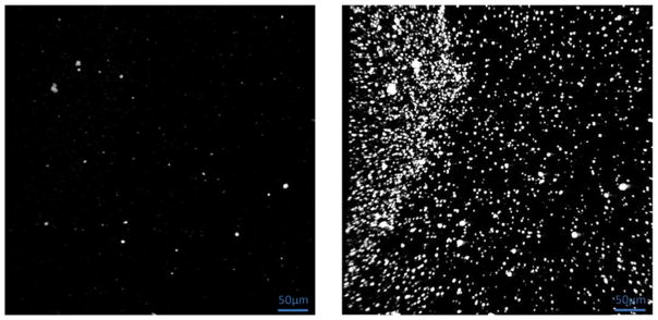
High dynamic range imaging. 4.5 orders of magnitude dynamic range were generated with 8.4 seconds acquisition. Each pixel was exposed to 512 laser pulses. Left and right panels are different representations of the same image, with the left linearly mapping the dynamic range to 8-bit grayscale and the right logarithmically to enhance the low intensity features.

Figure 3.

Peak height voltage histograms. Pixels with varying signal intensities were chosen. These are the histograms of the raw data used to calculate the average number of photons per laser pulse. The red curve exceeds the top of the graph and is about 3 times above the typical photon counting limit.

In routine operation, the histograms shown in Figure 3 are stored transiently in RAM on either the CPU or a GPU and analyzed in real time to produce a smaller output image, or image set, that can be written to the hard drive continuously. In this manner, the raw data throughput rates of > 3.2 GB/s can be processed in real-time to write files with outputs of a few kB/s.

In the present study, the relatively simple analysis approach described in the Theoretical Foundations section was used to assess whether binomial counting or signal averaging provided a S/N advantage, and record the preferred value in each pixel on a pixel-by-pixel basis. Because the binomial counting regime provides an absolute measure of photons, this approach also has the practical advantage of automatically calibrating the signal averaging results to report intensities in terms of photons/pulse (or photons/s), even well outside the photon counting regime.

The signals in this image spanned approximately 4.5 orders of magnitude in dynamic range, from a mean count rate of 1/512 up to 74 photons per laser pulse. The high limit approached the maximum voltage output of the PMTs used in these experiments, although efforts were made to remain below the fundamental saturation regime of the detector to avoid detector damage. The lower limit was set by the acquisition time and desired number of pixels for the image. An image acquisition time of 8.4s for a 512 by 512 pixel image allowed 512 laser pulses per pixel per incident polarization for two orthogonal polarizations. The dark counts for this detector were sufficiently low (nominally 30 per second with maximum gain) that the fundamental lower limit was near 4×10⁻⁷ photons/laser pulse, theoretically allowing over two hours per 512 by 512 image before the dark counts contributed an average of 1 count per pixel. If the intrinsic detector dark counts are used as a fundamental lower limit, the anticipated experimental linear dynamic range (LDR) spanned eight decades with a single detector and single data acquisition package. This assessment represents a lower bound on the LDR, as the impact of dark counts was further reduced by approximately an additional factor of ten by synchronous digitization, since only the dark counts coincident with laser pulses contributed to the detected background. These observations suggest an intrinsic dynamic range spanning ~10⁻⁸ photons/pulse to the measured high value of ~70 photons/pulse, or more than nine decades.

Although the present study is focused on dynamic range and S/N enhancement in quantitative nonlinear optical imaging, the basic architecture described in this instrument is well suited to a host of alternative measurement and data analysis approaches. By integrating GPU processing with high speed digitization, applications spanning polarization mapping to real-time dimension reduction approaches can be easily envisioned.

References

- 1.Nau VJ, Nieman TA. Photometric instrument with automatic switching between photon counting and analog modes. Analytical Chemistry. 1981;53(2):350–354. [Google Scholar]
- 2.Staton KL, Dorsel AN, Schleifer A. Large dynamic range light detection. Google Patents. 2002 [Google Scholar]
- 3.Kester WA. Data conversion handbook. Newnes. 2005 [Google Scholar]
- 4.Kissick DJ, Muir RD, Simpson GJ. Statistical Treatment of Photon/Electron Counting: Extending the Linear Dynamic Range from the Dark Count Rate to Saturation. Analytical Chemistry. 2010;82(24):10129–10134. doi: 10.1021/ac102219c. [DOI] [PMC free article] [PubMed] [Google Scholar]
- 5.Soukka JM, Virkki A, Hanninen PE, Soini JT. Optimization of multi-photon event discrimination levels using Poisson statistics. Optics Express. 2004;12(1):84–89. doi: 10.1364/opex.12.000084. [DOI] [PubMed] [Google Scholar]
- 6.Muir RD, Kissick DJ, Simpson GJ. Statistical connection of binomial photon counting and photon averaging in high dynamic range beam-scanning microscopy. Optics Express. 2012;20(9) doi: 10.1364/OE.20.010406. [DOI] [PMC free article] [PubMed] [Google Scholar]
- 7.Bevington PR, Robinson DK. Data Reduction and Error Analysis for the Physical Sciences. 3. McGraw Hill; Boston: 2003. [Google Scholar]
- 8.Blumenfeld D. Operations research calculations handbook. CRC; 2009. [Google Scholar]
- 9.Toth SJ, Madden JT, Taylor LS, Marsac P, Simpson GJ. Selective Imaging of Active Pharmaceutical Ingredients in Powdered Blends with Common Excipients Utilizing Two-Photon Excited Ultraviolet-Fluorescence and Ultraviolet-Second Order Nonlinear Optical Imaging of Chiral Crystals. Analytical Chemistry. 2012;84(14):5869–5875. doi: 10.1021/ac300917t. [DOI] [PMC free article] [PubMed] [Google Scholar]
- 10.Haupert LM, Simpson GJ. Screening of protein crystallization trials by second order nonlinear optical imaging of chiral crystals (SONICC) Methods. 2011;55(4):379–386. doi: 10.1016/j.ymeth.2011.11.003. [DOI] [PMC free article] [PubMed] [Google Scholar]
- 11.Muir R, Kissick DJ, Simpson GJ. Statistical Connection of Binomial Photon Counting and Photon Averaging in High Dynamic Range Beam-Scanning Microscopy. Opt Express. 2012;20:10406–10415. doi: 10.1364/OE.20.010406. [DOI] [PMC free article] [PubMed] [Google Scholar]