LONGITUDINAL INTENSITY NORMALIZATION IN THE PRESENCE OF MULTIPLE SCLEROSIS LESIONS

Abstract

This paper proposes a longitudinal intensity normalization algorithm for T₁-weighted magnetic resonance images of human brains in the presence of multiple sclerosis lesions, aiming towards stable and consistent longitudinal segmentations. Unlike previous longitudinal segmentation methods, we propose a 4D intensity normalization that can be used as a preprocessing step to any segmentation method. The variability in intensities arising from the relapsing and remitting nature of the multiple sclerosis lesions is modeled into an otherwise smooth intensity transform based on first order autoregressive models, resulting in smooth changes in segmentation statistics of normal tissues, while keeping the lesion information unaffected. We validated our method on both simulated and real longitudinal normal subjects and on multiple sclerosis subjects.

1. INTRODUCTION

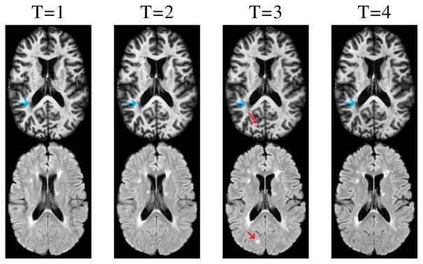
Magnetic resonance (MR) imaging is a popular noninvasive imaging modality used to image the structure of human brains, for applications such as understanding and following the progression of normal aging [1] or diseases like multiple sclerosis (MS) [2]. Analysis of a series of 3D images of a subject taken at different times is valuable since the images provide a time varying analysis of the soft tissues as well as biomarkers for the disease. However, the longitudinal changes of cerbro-spinal fluid (CSF), gray matter (GM), and white matter (WM) are of interest in both normal aging and diseases such as MS [3]. With MS, WM lesions are also present in addition to the healthy brain tissues. New lesions could persist, change volume, or disappear in later time points depending on the type and state of the MS and the lesion itself. An example is shown in Fig. 1 where four time-points (denoted by T) of magnetization prepared rapid gradient echo (MPRAGE) and T₁-w fluid attenuated inversion recovery (FLAIR) scans are shown for an MS subject. It can be seen that a lesion appears (red arrow) at the third time-point and is gone at the fourth. Other lesions (blue arrow) are present in all the scans. Accurate segmentations of such lesions as well as stable and smooth longitudinal segmentation of the normal tissues (i.e., CSF, GM, WM) are important for understanding the progression of disease.

Fig. 1.

MPRAGE (top) and FLAIR (bottom) scans for four time-points of an MS subject are shown.

Several 4D segmentation methods have been proposed in the past. A 4D formulation of the fuzzy c-means algorithm was proposed in [4]; it alternates between segmentation and a 4D registration between the corresponding segmentations of the time-points, thereby producing a longitudinally consistent segmentation. A 4D segmentation algorithm was also proposed to obtain consistent segmentations and cortical thicknesses of infant brains [5], where the segmentations of the later years are used as a prior to the first year and a novel 4D penalty is introduced on the cortical thickness measurements. These methods are tied to the particular choice of the segmentation and registration algorithms and can not be easily generalized. Also, these methods are usually aimed toward normal brains, where they are shown to provide longitudinally smooth segmentations and cortical thickness statistics. In this paper, we propose an intensity normalization method for subjects with MS lesions, that can be used as a pre-processing step to any segmentation method. We use a smooth auto-regressive (AR) model for the longitudinal transformation of intensities of the normal tissues of different time-points for T₁-w MPRAGE scans. We also use a prior for the lesions at each time-point, obtained from an atlas based topology preserving lesion segmentation method, called Lesion-TOADS [6], which takes both the MPRAGE and the FLAIR scans of a subject (e.g., Fig. 1) and provides fuzzy lesion memberships at every voxel. We validated our method on both phantom and a real longitudinal normal data by showing that the 4D normalization leads to stable and smooth longitudinal segmentations on normal tissues in the presence of MS lesions, keeping the lesion information unaffected, as MS lesions can disappear and reappear at random time-points. We compare our method with a landmark based normalization [7]. In the following section, we provide the mathematical model for the intensity normalization process.

2. METHOD

We assume that there are T time-points in a 4D dataset of an MS subject, consisting of MPRAGE and FLAIR scans at each time-point. We are interested in normalizing the intensities of the MPRAGE scans as they provide the most information about the structure of a brain. The FLAIR scans are used to obtain lesion information only. The 3D MPRAGE and FLAIR volumes at each time-point are denoted by and , t = 1, …, T, respectively. We assume that all ’s, t = 2, …, T, are rigidly registered to the baseline, , and similarly all ’s, t = 2, …, T, are rigidly registered to . Each is scaled by the maximum intensity of all the MPRAGE scans, such that the range of MPRAGE intensities is [0, 1]. Since all the images have the same domain, we denote the intensity of a voxel at the i^th location of as $y_i^{(t)}$, t = 1, …, T. For normal tissues, we assume that if the anatomy does not change over time, the intensity profile remains bounded, as seen from a deep WM and a ventricle voxel, shown in Fig. 2(a)–(d) with green and magenta lines. If the anatomy changes, such as growing ventricles, the intensities vary smoothly, as seen from the intensity profile of the voxel at the WM-ventricle boundary (blue). An AR(1) fit of the intensities of this voxel is also shown in red, indicating good approximation.

Fig. 2.

(a)–(c) shows three time-points of a normal longitudinal dataset [1]. Intensities of three voxels in (a), are plotted in (d), while an AR(1) fit of the intensities of the voxel at the WM-ventricle boundary is shown as a red line.

Our primary aim is to normalize the 4D intensities of an MS subject in such a way that the segmentations of the normal tissues become longitudinally smooth, while the lesions and their computed volumes remain unaffected, as the lesions are the primary biomarker of MS. To achieve this, we model the normal tissue voxels (i.e., largely CSF, GM, WM etc.) using an AR(1) process (as motivated by Fig. 2), while making sure that the voxels with lesions remain unchanged (as motivated by Fig. 1). This is formulated as,

$$\begin{array}{llll}{x}_i^{(t)}\hfill & =\hfill & m_i{x}_i^{(t-1)},\hfill & \text{if}{\ell }_{\mathrm{i}}=0\hfill \\ x_i^{(t)}\hfill & =\hfill & y_i^{(t)},\hfill & \text{if}{\ell }_{\mathrm{i}}=1.\hfill \end{array}$$ (1)

$x_i^{(t)}$ denotes the underlying normalized intensities at the i^th voxel, ℓ_i denotes an indicator function if the i^th voxel at any time-point is a lesion, m_i denotes the parameter of the AR(1) process. However, instead of using indicator functions, we use fuzzy memberships from Lesion-TOADS to provide a prior $w_i^{(t)}$ at each voxel. $w_i^{(t)}$ denotes the probability of observing a lesion at the i^th voxel at t^th time-point. We note that $w_i^{(t)}$ s are obtained using only FLAIR intensities, because it is seldom possible to obtain lesion information from T₁-w MPRAGE scans due to its similar contrast to GM. Thus, using the lesion priors, we reformulate Eqn. 1 using a combination of the priors, following a partial volume type model,

$$x_i^{(t)}=(1-w_i^{(t)})m_i{x}_i^{(t-1)}+w_i^{(t)}{y}_i^{(t)}.$$ (2)

From Eqn. 2, it can be seen that the underlying normalized intensities $x_i^{(t)}$ s follow an AR(1) process if the i^th voxel is not a lesion at any time-point, i.e., $w_i^{(t)}=0$, ∀ t, indicating normal tissue. If $w_i^{(t_1)}=1$ for some time-point t = t₁, the corresponding normalized intensity is the observed one $y_i^{(t_1)}$, indicating that the lesions are not being affected by the normalization. To fix boundary conditions at t = 1 and t = T, we first assume $x_i^{(0)}\equiv a_i$, and impose penalties at the boundaries such that $x_i^{(1)}\approx y_i^{(1)}$ and $x_i^{(T)}\approx y_i^{(T)}$.

Using an i.i.d. assumption on voxels, we propose to minimize the L₂ norm between the normalized intensities $x_i^{(t)}$ s and the observed intensities $y_i^{(t)}$ s and use higher penalty at the boundaries as,

$$E=\sum _{i\in \mathrm{\Omega }}\left\{\sum _{t=1}^T{\mathrm{\Lambda }}^{(t)}{(y_i^{(t)}-x_i^{(t)})}^2\right\},$$ (3)

where Λ = [λ, 1, …, 1, λ] is a vector consisting of weights on the L₂ errors for each time-point, with higher weight (λ > 1) on the first and the last time-point. Replacing Eqn. 2 in Eqn. 3, the energy functional becomes a function of the AR parameters m_i and the normalized intensities a_i’s as,

$$E=\sum _{i\in \mathrm{\Omega }}\left\{\sum _{t=1}^T\left[{\mathrm{\Lambda }}^{(t)}{(1-w_i^{(t)})}^2{(y_i^{(t)}-m_i^{t-1}{a}_i)}^2\right]\right\},$$ (4)

The $w_i^{(t)}$’s are obtained from Lesion-TOADS at each time-point. Eqn. 4 is minimized w.r.t. m_i by finding roots of a (2T − 1)^th order polynomial

$$m_i:\sum _{t=1}^T{\mathrm{\Lambda }}^{(t)}{(1-w_i^{(t)})}^2(t-1)(y_i^{(t)}-m_i^{t-1}{a}_i)m_i^t=0.$$ (5)

Similarly, a_i is obtained from

$$a_i=\frac{{\sum }_{t=1}^T{\mathrm{\Lambda }}^{(t)}{(1-w_i^{(t)})}^2{y}_i^{(t)}{m}_i^{t-1}}{{\sum }_{t=1}^T{\mathrm{\Lambda }}^{(t)}{(1-w_i^{(t)})}^2{m}_i^{2t-2}}.$$ (6)

Once m_i and a_i are found for each i ∈ Ω, the normalized intensities are obtained from Eqn. 2. In all our experiments, we empirically choose λ = 3.

3. RESULTS

3.1. Validation

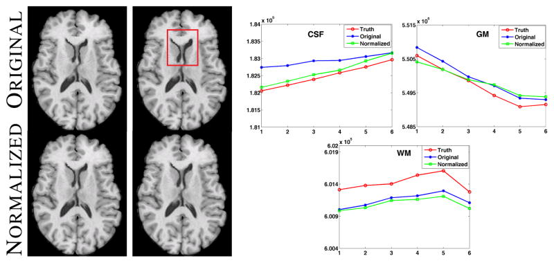
We first validate the effect of the smoothly varying normalization part, i.e., the AR(1) process, on normal data by simulating atrophy near the ventricle. We generated eight time-points of a normal subject using different atrophy radii [8], simulating normal aging where ventricles tend to grow in size. The tissue contrast in the images are kept same while the ventricles are deformed. The second and sixth time-points are shown in Fig. 3 (top row). The region of atrophy is shown by the red box. Then the normalization is performed assuming $w_i^{(t)}=0$, ∀ t, ∀ i, as shown in Fig. 3 bottom row. The images are segmented with a 3-class Gaussian mixture model and the hard segmentations are compared with the 3-class true segmentations provided by the atrophy simulation algorithm itself. The plots in Fig. 3 right panel show the volumes (in voxels) of 3 tissues, namely CSF, GM, WM, plotted against the time-points. The tissue volumes after normalization have a similar trend as the truth as well as the trend shown by original images. Our normalization tends to smooth the intensity profile, indicating small decrease in WM volume. Although we lose a little sensitivity that way, but as shown in the subsequent results, the gain in stability is significant.

Fig. 3.

Left panel shows original images with atrophy and the corresponding normalized images. The right panel shows the volumes (in voxels) of CSF, GM and WM for eight time-points, obtained from the hard segmentations of the truth (red), original images (blue) and the normalized ones (green).

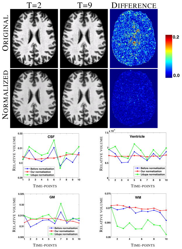
Next we experiment on MPRAGE scans of a normal subject acquired in ten consecutive weeks. As before, by assuming $w_i^{(t)}=0$, the lesion priors are not used. As the data is taken weekly, we should expect very little or no variation in the longitudinal tissue volumes. Fig. 4 top row shows the 2^nd and the 9^th time-points of the subject, along with the normalized images in the second row. To show segmentation stability quantitatively, the relative volumes of four normal tissues, CSF, GM, WM, and ventricles, are found using an atlas based segmentation [9] and plotted in Fig. 4 third and bottom rows. Visually, the variation is smaller after 4D normalization (red curves) in comparison with the original images and the landmark based normalization [7]. The coefficient of variations (CV) for the 4 tissues before normalization are [0.0126, 0.023, 0.006, 0.005], while they become [0.004, 0.003, 0.003, 0.002] after 4D normalization. Comparing ours with the landmark based method, t-tests give p-values < 0.05 for the null hypothesis that the differences in CV are the same between our method and [7] as well as between our method and the original ones, indicating significant improvement in the stability of the longitudinal segmentation in the absence of lesions.

Fig. 4.

Original and normalized images of two time-points of 10 weekly scans of a normal subject and the corresponding difference images. Bottom two rows show the relative volumes of CSF, GM, WM, and ventricles plotted against the time-points.

3.2. Experiment on MS data

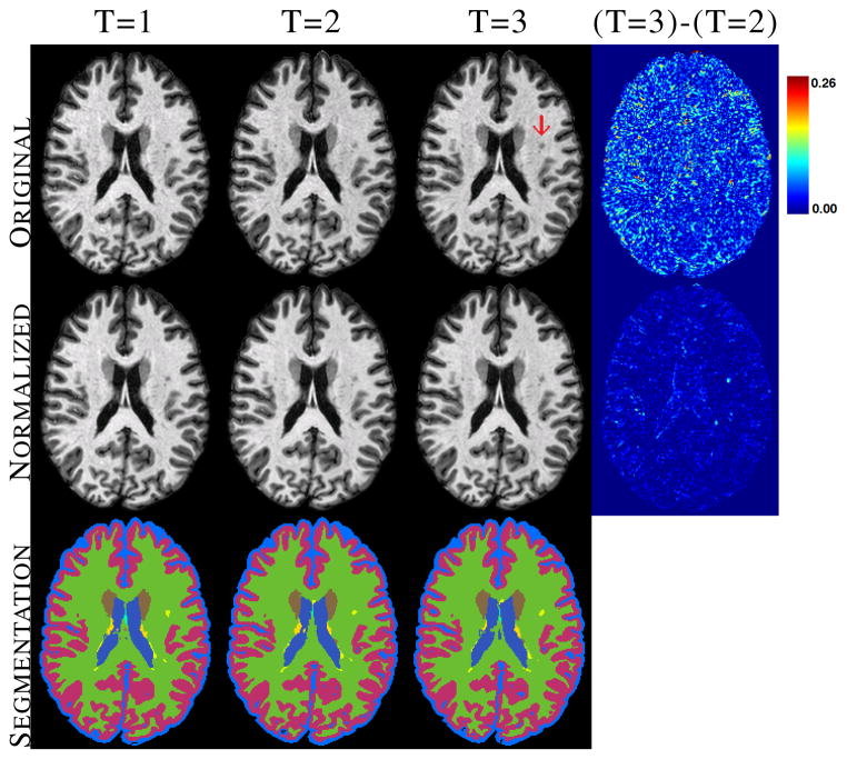
In this section, we show the effect of longitudinal segmentation on both normal tissues and lesions for 16 MS subjects, having 3–5 time-points each, approximately separated by a year. Every subject has a 3D MPRAGE and a FLAIR acquisition of size 218×262×170, with 0.828×0.828×1.1mm³ resolution. Each time-point, t = 2, …, T, is rigidly registered to the first year MPRAGE. Using the MPRAGE and the FLAIR scans, we first find the lesion priors $w_i^{(t)}$ s, then normalize the MPRAGE scans using the lesion priors using Eqn. 5 –6. Three time-points of a subject are shown in Fig. 5 top row, along with the whole brain segmentations before and after normalization. As seen from the absolute difference image of the third and second time-points, 4D normalization reduces the difference in intensities significantly, although lesion intensities are preserved, shown using a red arrow.

Fig. 5.

Original and normalized MPRAGE scans of an MS subject, along with the corresponding whole brain segmentations of the normalized image for the major tissues are shown. Lesions are shown in yellow.

To show the quantitative improvement in segmentation stability, we report mean and standard deviation of CVs in Table 1, averaged over 16 MS subjects. A t-test shows that the CVs are significantly reduced (p-value < 0.01) after 4D normalization for CSF, GM, and ventricles compared to the original images as well as the landmark based normalization, indicating more stable longitudinal segmentation. An F-test assuming the null-hypothesis that the lesion volumes are the same before and after normalization gives a p-value > 0.05, indicating no significant change. We plot the relative volumes of the tissues as well as lesions w.r.t. the time-points in Fig. 6 for the subject shown in Fig. 5. Evidently, the segmentations for normal tissues (such as ventricle and GM) have become more stable, with a gradual increase in ventricles and decrease in GM, (CV 0.031 compared to 0.044 for ventricles), as expected in MS [3]. Also the lesion segmentation remains unaffected, as seen visually. Here we mention that the normalized images visually look more smooth than the original ones, which is the result of the AR(1) smooth regression.

Table 1.

Coefficients of variations of relative volumes of four tissues before and after ours and landmark based normalization, denoted by LM.

	CSF	Ventricle	GM	WM
Before	0.033±0.012	0.041±0.019	0.014±0.007	0.011±0.006
LM	0.037±0.014	0.039±0.019	0.015±0.006	0.016±0.016
4D	0.027±0.013	0.032±0.019	0.011±0.006	0.010±0.007

Bold indicates statistically significantly smaller than the other two (p-value < 0.05).

Fig. 6.

GM, ventricle, and lesion relative volumes plotted against the time-point for two subjects. Dotted line indicates the one shown in Fig. 5.

4. DISCUSSION AND CONCLUSION

We have proposed a novel 4D intensity normalization frame-work for T₁-w MPRAGE images. The method takes into account the lesion information and produces stable longitudinal segmentations of normal tissues while keeping the lesion information unaffected. In the future, we will incorporate FLAIR intensities in the normalization process to have more robust normalization.

References

- 1.Resnick SM, Goldszal AF, Davatzikos C, Golski S, Kraut MA, Metter EJ, Bryan RN, Zonderman AB. One-year age changes in MRI brain volumes in older adults. Cerebral Cortex. 2000;10(5):464–472. doi: 10.1093/cercor/10.5.464. [DOI] [PubMed] [Google Scholar]
- 2.Ozturk A, Smith SA, Gordon-Lipkin EM, Harrison DM, Shiee N, Pham DL, Caffo BS, Calabresi PA, Reich DS. MRI of the corpus callosum in multiple sclerosis: association with disability. Multiple Sclerosis. 2010;16(2):166–177. doi: 10.1177/1352458509353649. [DOI] [PMC free article] [PubMed] [Google Scholar]
- 3.Fisher E, Lee J-C, Nakamura K, Rudick RA. Gray matter atrophy in multiple sclerosis: a longitudinal study. Annals Neurol. 2008;64(3):255–265. doi: 10.1002/ana.21436. [DOI] [PubMed] [Google Scholar]
- 4.Xue Z, Shen D, Davatzikos C. CLASSIC: Consistent Longitudinal Alignment and Segmentation for Serial Image Computing. NeuroImage. 2006;30(2):388–399. doi: 10.1016/j.neuroimage.2005.09.054. [DOI] [PubMed] [Google Scholar]
- 5.Wang L, Shi F, Yap PT, Gilmore JH, Lin W, Shen D. 4D Multi-Modality Tissue Segmentation of Serial Infant Images. PLoS One. 2012;7(9):e44596. doi: 10.1371/journal.pone.0044596. [DOI] [PMC free article] [PubMed] [Google Scholar]
- 6.Shiee N, Bazin PL, Ozturk A, Reich DS, Calabresi PA, Pham DL. A topology-preserving approach to the segmentation of brain images with multiple sclerosis lesions. NeuroImage. 2010;49(2):1524–1535. doi: 10.1016/j.neuroimage.2009.09.005. [DOI] [PMC free article] [PubMed] [Google Scholar]
- 7.Nyul LG, Udupa JK. On Standardizing the MR Image Intensity Scale. Mag Res in Medicine. 1999;42(6):1072–1081. doi: 10.1002/(sici)1522-2594(199912)42:6<1072::aid-mrm11>3.0.co;2-m. [DOI] [PubMed] [Google Scholar]
- 8.Karacali B, Davatzikos C. Simulation of tissue atrophy using a topology preserving transformation model. IEEE Trans Med Imag. 2006;25(5):649–652. doi: 10.1109/TMI.2006.873221. [DOI] [PubMed] [Google Scholar]
- 9.Bazin PL, Pham DL. Topology-preserving tissue classification of magnetic resonance brain images. IEEE Trans on Medical Imaging. 2007 Apr;26(4):487–496. doi: 10.1109/TMI.2007.893283. [DOI] [PubMed] [Google Scholar]