eALPS: Estimating Abundance Levels in Pooled Sequencing Using Available Genotyping Data

Abstract

The recent advances in high-throughput sequencing technologies bring the potential of a better characterization of the genetic variation in humans and other organisms. In many occasions, either by design or by necessity, the sequencing procedure is performed on a pool of DNA samples with different abundances, where the abundance of each sample is unknown. Such a scenario is naturally occurring in the case of metagenomics analysis where a pool of bacteria is sequenced, or in the case of population studies involving DNA pools by design. Particularly, various pooling designs were recently suggested that can identify carriers of rare alleles in large cohorts, dramatically reducing the cost of such large-scale sequencing projects. A fundamental problem with such approaches for population studies is that the uncertainty of DNA proportions from different individuals in the pools might lead to spurious associations. Fortunately, it is often the case that the genotype data of at least some of the individuals in the pool is known. Here, we propose a method (eALPS) that uses the genotype data in conjunction with the pooled sequence data in order to accurately estimate the proportions of the samples in the pool, even in cases where not all individuals in the pool were genotyped (eALPS-LD). Using real data from a sequencing pooling study of non-Hodgkin's lymphoma, we demonstrate that the estimation of the proportions is crucial, since otherwise there is a risk for false discoveries. Additionally, we demonstrate that our approach is also applicable to the problem of quantification of species in metagenomics samples (eALPS-BCR) and is particularly suitable for metagenomic quantification of closely related species.

1. Introduction

Over the past several years, genome-wide association studies (GWAS) have identified hundreds of common variants involved in dozens of common diseases (Manolio et al., 2008). These discoveries leveraged technological advances in genotyping microarrays (Matsuzaki et al., 2004; Gunderson et al., 2005), which allowed for the cost-effective collection of common genetic variation in large numbers of individuals. More recently, technological advances in high-throughput sequencing (HTS) technologies have rapidly decreased the cost of sequencing cohorts of individuals (Wheeler et al., 2008). The advantage of sequencing technologies relative to genotyping technologies is that sequencing technologies collect both rare and common variation providing the opportunity for implicating rare genetic variation, in addition to common variation, in human disease.

Unfortunately, to identify disease associations with rare variants, the cohorts that must be sequenced consist of thousands of samples. Even when considering the decrease in costs over the past decade, the cost of sequencing these cohorts is prohibitively expensive. The actual cost of sequencing a sample consists of two parts. The first part is the cost of preparing a DNA sample for sequencing, which we refer to as the library preparation cost. Library preparation is also the most labor-intensive part of a sequencing study, and though newer technologies (Coupland et al., 2012) promise to make this stage unnecessary, sequence yields of such methods are still an order of magnitude smaller than more established sequencing techniques, preventing them from being applied cost effectively to large studies. The second part is the cost of the actual sequencing, which is proportional to the amount of sequence collected, which we refer to as the sequencing per-base cost. Technological advances are rapidly reducing the per-base cost of sequencing while the library preparation costs are more stable. A recently proposed approach to reduce the overall sequencing cost and to avoid potential biases introduced during library preparation is to utilize sequencing pools. The basic idea behind this approach is that DNA from multiple individuals is pooled together into a single DNA mixture, which is then prepared as a single library and sequenced. In this approach, the library preparation cost is reduced because one library is prepared per pool instead of one library per sample. DNA pooling has been successfully applied to GWAS data that reduces costs by one or two orders of magnitude (Skibola et al., 2010; Brown et al., 2008; Hanson et al., 2007). However, pooling DNA from a large number of individuals can introduce a great deal of background noise in the data that may reduce the reliability of and increase the difficulty in the downstream analysis. In contrast to pooling strategies in GWAS data where a small number of pools are genotyped—each consisting of a large number of samples—in sequencing pooling studies, typically a small number of individuals are sequenced in each pool, making the noise amenable to explicit modeling. Moreover, DNA pooling has been successfully applied to next generation sequencing (Erlich et al., 2009; Hormozdiari et al., 2012), where they ran a large pooling study for the identification of rare mutations in bacterial communities.

Recent work in the area (Golan et al., 2012; Prabhu and Pe'er, 2009) has focused mainly on effective designs of pooled studies that can reduce the number of pools required for the detection of causal variants. In addition, suggested association statistics for rare SNP analysis typically involve the comparison of the total number of rare mutations in the cases and controls, therefore, there is no need for individual sequencing in such cases. Indeed, in this work we use as a benchmark a sequencing study of non-Hodgkin's lymphoma (NHL), where the samples have been partitioned into sets of five samples, and each set was pooled and whole-genome sequenced. The latter study is currently ongoing, and without the tools presented in this article, the study might result in false discoveries. Generally, such designs allow for an increased statistical power due to the increase in sample size. However, the analysis of these studies relies on the assumption that the pools are perfectly constructed, meaning that the fraction of DNA from each sample is known; typically, each DNA mixture contains an exact amount of DNA information intended from each individual in the pool. As we show using real experimental data from NHL, this assumption is wildly inaccurate, and the amount of DNA in each mixture is often different from the intended amount. This might potentially lead to both false positives and reduced statistical power.

In this article, we present a computational methodology to infer the relative abundance or the fraction of each individual in the DNA mixture of a pool directly from the sequencing data, given that we have a small amount of genotyping data for the individuals. This assumption is applicable in many cases, particularly since most current sequencing studies are being performed on cohorts where a genome-wide association study has been previously performed. Our method can be applied directly to the data obtained from a pool sequencing study as the first step in the analysis. We present a formal statistical framework for the estimation of relative abundances, taking into account the presence of sequencing and genotyping errors. In practice, reliable genotypic data of all pooled samples might not be available due to separate quality control procedures for sequencing and genotyping. We therefore propose an extension that handles missing genotypic data by leveraging the linkage disequilibrium structure of the genome. We demonstrate using real data that a naive analysis without applying our method would lead to false positive associations.

The computational problem of estimating the relative abundances in DNA pools is closely related to the computational problem of estimating the abundance of species in metagenomic samples. Bacteria are vital for humans, affecting a wide range of food and health industries. Known to reside in the human body in numbers higher than the number of human cells (Savage et al., 1968), the set of bacteria and their interactions are an indication of the physical condition of a person and were shown to be correlated with various diseases (Guarner and Malagelada, 2003; Heselmans et al., 2005; Mahida, 2004). In 2008, the National Institute of Health (NIH) launched the Human Microbiome Project (HMP) to examine all existing microorganisms in the human body. Following the HMP, another project named Metagenomics of the Human Intestinal Tract project (MetaHIT) was launched with the goal of studying gut bacteria. Both projects aim to increase our knowledge of bacterial community effects on our body. The first step, however, is to understand which bacteria are available in each sample and the fraction of each bacterium. The latter problem is mathematically very similar to the estimation of DNA fractions in a pooled sample, and we therefore apply our methods to metagenomic instances (eALPS-BCR).

Bacterial fraction estimation in the context of metagenomics has already been addressed by Amir and Zuk (2011), who used an approach based on Sanger-sequencing of a highly preserved genomic region (16S) found in all bacteria. They obtain a sequence-based profile of the bacterial community in that region and use a compressed sensing (CS) framework to compute the fraction of each bacterium in the sample. Due to its decreasing cost and increasing throughput, high-throughput sequencing (HTS) has also been widely applied to metagenomic samples to infer species abundance (Hamady et al., 2008; Dethlefsen et al., 2008; Angly et al., 2009; Xia et al., 2011). The kind of data generated by a single Sanger-sequencing reaction is very different from HTS data, and the compressed sensing approach is not specifically designed for such data. Therefore, methods such as GAAS (Angly et al., 2009) and GRAMMY (Xia et al., 2011) are based on similarity scores of high-throughput sequencing reads that are mapped to a database of known bacterial genomes. Examination of whole-genome reads as opposed to a single highly preserved region is more suitable to the analysis of homogeneous bacterial communities, considering that very few mutations might be present in the 16S region of closely related species. In general, the problem of estimating relative abundances becomes increasingly difficult in lower taxonomic levels and is particularly hard when considering strains of the same species. We show that with minor adjustments, our method (eALPS-BSR) can be directly applied to HTS data, and argue that modeling of linkage-disequilibrium patterns of bacteria greatly improves estimation accuracy in such scenarios. Finally, we bring experimental results on various simulated arrangements of bacterial communities.

2. Methods

2.1. Description of the data-generating process

We first set the stage by describing a mathematical model for the generation of sequencing data in a pooling scheme. As always, the model might be an oversimplified abstraction of reality, however, in the Results section we show that our estimates are highly accurate on real data, and we therefore argue that the model approximates to an adequate degree the realistic mechanism of sequencing data generation.

Consider a scenario in which the DNA of N individuals is pooled and then sequenced. In addition, assume that these N individuals have genotype information in M positions, described by a matrix H_N×M, where is the minor allele count of the i-th individual in the j-th position. Such a scenario may appear in pooled sequencing studies, such as the one we describe in the Results (for non-Hodgkin's lymphoma), or in scenarios where a set of DNA pools is used to detect rare variants (such as in Lin et al., 2011; Price et al., 2010; Lee et al., 2011). In addition, as we discuss below, this scenario also occurs in metagnomic analysis where a set of bacteria are sequenced together.

Ideally, at least in the case of human studies, one would aim at specific relative abundances for each of the samples, which are typically equal amounts of DNA for each sample, but in some cases there are other designs (e.g., Golan et al., 2012). However, in practice the actual relative abundances may be quite different from the desired levels. Particularly, we demonstrate in the Results section that for some pools with presumably equal amounts of DNA from each individual, the actual fractions of the samples often deviate considerably, and this has to be taken into account in any subsequent analysis.

We denote the unknown relative abundances , where α_i is the relative abundance of the i-th individual. The pooled sample undergoes high-throughput sequencing, resulting in the collection X = {x_j}, where every x_j is a vector of length t_j (the coverage at position j), and the elements x_jr represent the minor/major allele status of the r-th read in the j-th position:

We assume that for each position j, the number of reads t_j in that position is generated from a Poisson distribution with some parameter C, the mean coverage over the entire genome. The reads for every position are then distributed according to a mixture of N Bernoulli distributions with parameters , the mixture weights being the relative abundances . Formally, our model assumes that a read x_jr is generated by randomly picking an individual i according to the proportions and assigning the allele status 0/1 according to the minor allele probability h_ij. To specify the identity of the mixture components, we introduce the (unknown) latent variables Z = {z_ijr}, where z_ijr are indicator functions that determine the individual every read originated from, that is,

We model the sequencing technology as an error-prone process, with a probability ɛ for a sequencing error that switches the read from minor to major or vice versa. Thus, in our model, the unknown parameters of the model are α, ɛ and H, and the observed data is X. We are mostly interested in α in this article, although we also show how to estimate . Under this model, the likelihood of the data is given by:

(1)

where p_i(x_jr|ɛ) is the probability to observe read x_jr given that it originated from individual i and with sequencing error ɛ, thus: .

It is important to note that the likelihood formulation in (1) relies on the assumption that reads do not span more than a single variant. In reality, this is of course not the case, but occurrences of closely positioned SNPs are infrequent enough as to allow us to overlook this possibility without substantially undermining the correctness of our model. Given the genotypes, the reads x_jr are therefore generated independently across the different positions in the genome, as they only depend on the value of h_j. In the case where some of the genotypes are unknown (as discussed below), this is not true and should be addressed properly.

2.2. Relative abundance estimation

We now present the algorithm for estimation of relative abundances in the full genotypic data scenario (eALPS), where genotypes of all N sequenced individuals are given. Our objective is to find a maximum-likelihood estimate of the model parameters, that is, the relative abundances α and the sequencing error ɛ. Since Z is unknown, we use an expectation-maximization (EM) approach, which, instead of trying to maximize the likelihood given in Equation (1), considers the marginal likelihood of the observed data as follows:

(2)

The EM algorithm is an iterative algorithm, where in each iteration the algorithm searches for parameters that maximize the expected value of the marginal log-likelihood function given a current estimate of the parameters. This procedure is repeated until a convergence of either the log-likelihood or the parameters is achieved. Following the standard notation for EM, we call this quantity the Q-function (i.e., the marginal log-likelihood function), and write it as:

(3)

where . The maximization over α involves only the first term in Equation (3), which is clearly a concave function of α and can be solved easily using Gibbs' inequality while enforcing the constraint that . Finding a closed form expression for ɛ^(t+1) is not possible, however, simple numerical methods such as gradient descent can be applied to produce the next estimate for the sequencing error. The update rules are then:

2.3. Missing genotypes

In practice, it is often the case that genotype information is only available to a subset of the data, specifically to the samples that were previously genotyped for a genome-wide association study in the pre-high-throughput sequencing era. Moreover, even in the case where all individuals are genotyped, some of the SNPs are not called for some of the individuals, and in such cases our approach is not applicable. We therefore developed an improved method that can handle missing genotype data without compromising the accuracy of estimated parameters. Formally, suppose that for a pool of N individuals, we have only N′ < N genotyped individuals, and we wish to estimate the relative abundances given the observed genotypes and the observed read counts X as in the previous section. Regarding the true genotypes H as a set of latent variables in addition to Z, we can follow a similar derivation of the EM algorithm to maximize the new likelihood function as follows:

Maximization of this likelihood function can be achieved in a similar fashion to the previous case in which all genotypes are known, with the expectation step involving an extra iteration on all possible realizations of the missing genotype. This approach, however, fails to take into account the presence of linkage disequilibrium (LD) between adjacent loci, which renders invalid the assumption of independence between the h_j's, producing suboptimal estimates of the model parameters. Particularly, we show in the Results section that this method (eALPS-MIS) systematically underestimates the relative abundances of the missing individuals.

Fortunately, leveraging the information of LD available in population samples, as well as the known genotypes themselves, allows for very accurate estimations of the conditional probability of the latent variable H, given the observed data and the current estimate of the parameters. In fact, when LD information is utilized, most possible values of h_ij have negligible probabilities and can be omitted from the expectation step. We continue to show that even a hard assignment of h_j to the most likely value in every iteration of the EM algorithm conserves its desirable convergence properties.

The algorithm we propose (eALPS-LD) therefore uses the following scheme: Given a current estimate of the parameters α and ɛ, find a maximum likelihood estimate for the missing genotypes h_ij, N′ < i ≤ N, using the LD model that will be described shortly. Using this estimate of h_ij, continue the EM iteration as in the previous EM derivation for known genotypes, that is, calculate the expectation over the latent variables (Z) and maximize the log-likelihood function. This approach can be justified from a statistical point of view using the same arguments presented in Neal and Hinton (1998). The hard assignment of h_j is also computationally advantageous, as it eliminates the need for an exhaustive enumeration of all realizations of possible genotypes.

To find the most likely missing genotype, we need to model population haplotype frequencies, and we do so using a Markov model with a similar structure to those recently used by Kimmel and Shamir (2005;), Kennedy et al., (2008), and Browning (2006). The basic structure of this LD model is that of a left-to-right directed graph, with M disjoint sets of nodes corresponding to the M loci. Edges in the directed graph correspond to the transition probabilities and only connect nodes in consecutive sets. Every node in the graph corresponds to one of the two possible alleles, with potentially multiple nodes representing each allele in a specific locus, allowing for multiple haplotypes (more accurately, haplotype clusters) with the same allele in that position to be represented. The edges carry the population frequency of transition from a haplotype in one position to a haplotype in the next position, meaning that every haplotype in the population corresponds to a path in the graph. Training of the model according to population samples can be done either with the Baum-Welch algorithm for HMMs, like in Kennedy et al. (2008), or in the constructive approach described in Browning (2006). In our implementation, we used the BEAGLE genetic analysis software package (version 3.3.2) to build the LD model.

We now turn to define the full model used to infer the missing genotypes, with the above LD model as a basic building block. In the interest of simplicity, we consider the case in which only one genotype is unobserved, though a straightforward extension to handle multiple missing genotypes is applicable. The overall model is a hidden Markov model composed of two copies of the LD model, that is, every state is represented by a pair (q₁, q₂) with q₁ expressing the first haplotype and q₂ the second haplotype of the missing genotype. Assuming the Hardy–Weinberg equilibrium, the two haplotypes of the missing genotype are independent, therefore the transition probabilities are simply the product of the frequencies carried by each of the corresponding edges in the LD model. Each node in the HMM emits the minor allele read count of that position, c_j, with probability where . The posterior probability of every possible haplotype can be computed using the standard forward–backward algorithms in O(MS²E²) time, where S is an upper bound on the number of states for each position in the basic LD model, and E is an upper bound on the indegree of nodes in the graph (i.e. number of incoming edges). Recall that edges in the graph connect only those nodes lying on a path that represents a haplotype in the reference population, therefore E is expected to be a small number.

An important quality of LD models trained by either of the two approaches mentioned previously deals with the indegree of nodes in the graph in view of the fact that the complexity of the forward–backward algorithm depends on it. While a trivial upper bound for E would be S², we observe that the number of edges carrying non-negligible transition probabilities is strictly bounded by the total number of different haplotypes in the reference panel used to build the model. The actual number depends on the model complexity, tuned by the maximum number of nodes we allow in every position, denoted earlier by S. For a specific reference panel, increasing S means that E will decrease. A typical LD model trained using the BEAGLE software package on reference panels of Europeans from HapMap yields a maximal indegree of 5 (with an average of 1.8). The overall complexity of the eALPS-LD algorithm can therefore be considered to be O(CS²M), with a small constant C.

2.4. Bacterial community reconstruction

The estimation of relative abundance levels in DNA pools is naturally applicable to metagenomic analysis, particularly to the reconstruction of bacterial communities. Given a mixture of known bacteria, the goal of bacterial community reconstruction (BCR) is to detect which bacterial species are present in the sample and to estimate their fractions. Early metagenomic studies accomplished this task by screening of environmental libraries for the presence of known markers in ribosomal genes and subsequent sequencing of clones of interest. Specifically, these methods typically exploit the 16S region, which is a highly conserved 1.5kb segment found in all known bacteria. Shown to be effective in reconstruction of various bacterial communities (Amir and Zuk, 2011), this approach is appropriate for distinguishing between species at large evolutionary distances, as it depends strongly on slow-evolving genes. Reconstructing a community containing closely related organisms, for example same-species strands in a microbial gut sample, is bound to fail if analysis is limited to conserved regions alone. As the ability to distinguish between different species diminishes with increasing interrelatedness, considerably longer genomic segments need to be analyzed.

Analyses of high-throughput sequencing data with the purpose of assigning the read sequences to their taxonomic units can be categorized to signature-based binning and mapping-based classification approaches, the former employing the DNA base compositional asymmetries (e.g., GC content) of bacterial genomes as a unique identifier of different taxonomic units, and the latter attempting to find similarities to reference sequences. Where datasets of closely related reference genomes are available, the second approach is particularly useful, with the potential of being significantly more precise. Though still quite limiting, the availability of suitable reference sequences to map to is becoming less of an issue, as targeted sequencing of yet unsequenced taxa and large-scale metagenome projects start to deliver large quantities of microbial genomes at an increasing pace.

Recently, a novel method (GRAMMy) based on high-throughput sequencing of the entire genome was introduced in Xia et al., (2011) and tested on various standard datasets. Somewhat similar in character to the method in this article, the authors consider the metagenomic reads as arising from a finite mixture model, where the mixing parameters are the relative abundances and the component distributions of reads are approximated using k-mer frequencies in the reference genomes. Expectation-maximization is then applied to estimate the mixing parameters. We hereby propose an efficient method based on common SNPs in orthologous genes that eliminates the necessity to handle whole-genome read data, and focuses only on the highly informative SNPs that reside in homologous genes. A major benefit of this approach is that it allows, in the same manner as with human genomes, to take advantage of existing LD structure in closely related bacteria to account for possibly unknown species of bacteria in the sample.

Suppose we have N sequences of known bacteria that we wish to use as references and a metagenomic sample that is sequenced to produce short reads. To be able to use the same formulation as before for this setting, a preprocessing step is performed on the bacterial reference genomes. First, genes that are homologous in all N genomes are extracted and aligned against an arbitrarily selected reference genome. Subsequently, SNP calling is performed on the aligned regions resulting in a set of M SNPs. The total number of SNPs we will acquire in this procedure depends on the similarity of the reference genomes—high relatedness of the samples means more orthologs, albeit fewer variants in every single gene. BCR thus reduces to the previously presented problem of relative abundance estimation: We regard the available database of orthologous regions as the collection of true genotypes present in the sample.

3. Results

3.1. Non-Hodgkin's lymphoma dataset

Our method was applied to a real population study of non-Hodgkin's lymphoma (NHL) for which genome-wide association data were available. In this dataset, a whole-genome sequencing on a group of lymphoma cases was conducted, with the aim of identifying additional common and rare lymphoma associated variants undetected by previous genome-wide association studies (GWAS). The studied samples consisted of a subset of follicular lymphoma samples that were part of a recent GWAS conducted in the San Francisco Bay Area. Full details of the GWAS, including the process and criteria for subject selection, genotyping, quality control, and statistical analysis, have been described elsewhere (Conde et al., 2010). A total of 312,768 markers genotyped in 1,431 individuals passed the quality control criteria and were used for genome-wide association analysis. Among the follicular lymphoma cases for which GWAS data was available, 155 were used in this study. To construct each pool, equal amounts of DNA (1,320 ng) were combined from five individuals of the same sex and age in a total volume of 110 uL. Importantly, we demonstrate below that in reality the amounts of DNA were not equal even though the pooling protocol aimed at exact amounts of 1,320 ng of DNA from each pool. Sequencing was outsourced to Illumina FastTrack Services (San Diego, CA). gDNA samples were used to generate short-insert (target 300 bp) paired-end libraries, and a HiSeq2000 instrument was used to generate paired 100 base reads according to the manufacturer instructions. The software ELAND was used for sequence alignment, and the coverage was 35 per base for the pool, thus 7 per base for each sample.

3.2. Simulated data

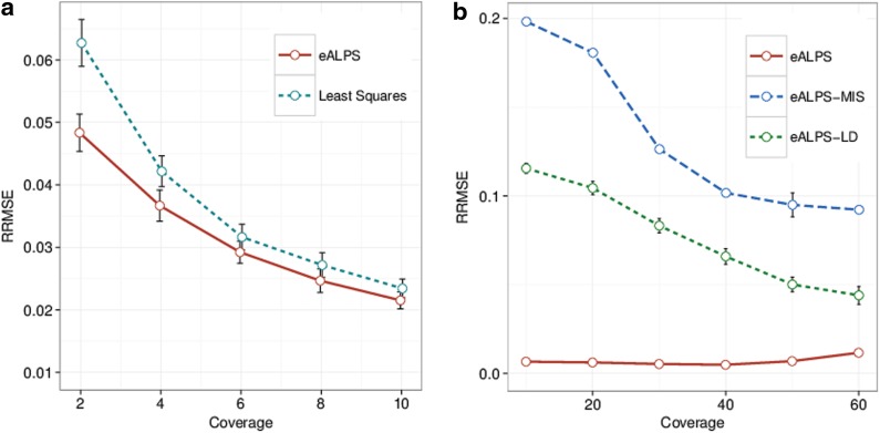
We used the non-Hodgkin's lymphoma genotype data as a starting point in order to simulate data according to the following model. We assume that the genotype values g_ij are given by the non-Hodgkin's lymphoma genotype data. Then, for every position we draw a random sample t_j (the total number of reads covering the j-th SNP) from a Poisson distribution Pois(T), where the mean is equal to the desired coverage T. The minor allele counts, c_j are then drawn from a binomial distribution B(t_j,∑_iα_i((1 − ɛ)g_ij + ɛ(1 − g_ij))), and the major allele counts are just t_j − c_j. We calculate the root mean squared error (RMSE) of the predicted α and compare to a simple least square estimation of the relative abundances. Results for this comparison are shown in Figure 1. The least-squares method is based on the assumption of normally distributed noise, which is clearly violated for low coverage sequencing. Indeed, we observe that least squares tends to perform poorly as the coverage goes down, while our method (eALPS) achieves significantly better performance in coverages lower than 4X.

FIG. 1.

Relative abundance estimations in simulated pools with five individuals using 230,000 SNPs. (a) Assuming all five genotypes are known. (b) Assuming one of the indviduals' genotypes is missing. The methods compared are: eALPS, full genotypic data; eALPS-LD, missing genotype and utilizing LD; eALPS-MIS, missing genotype and full (soft) EM. SNP, single-nucleotide polymorphism; LD, linkage disequilibrium; EM, expectation-maximization.

We note that the least squares estimation is only applicable when all individuals have genotype information. We also explored the scenario in which at least one of the individual's genotype is unknown. Particularly, we randomly picked one of the pools that has full genotype data, generated major and minor allele counts as mentioned in the previous experiment, and compared the performance of the full genotypic data method (eALPS) to the methods discussed in Section 2.3 (eALPS-MIS and eALPS-LD) when one of the individuals' genotype data is omitted. We examined the effect of different coverages and the number of sampled SNP on the RMSE measured, summarized in Figure 1. Evidently, utilizing the linkage disequilibrium information considerably improves the accuracy as observed by comparing the performance of eALPS-MIS and eALPS-LD.

3.3. Results on real data

In order to obtain a realistic characterization of the parameters used in our simulations, that is, sequencing error rate and distribution of relative abundance levels, we evaluated the eALPS method on the real sequencing data obtained by the non-Hodgkins lymphoma (NHL) study.

3.3.1. Complete genotype information

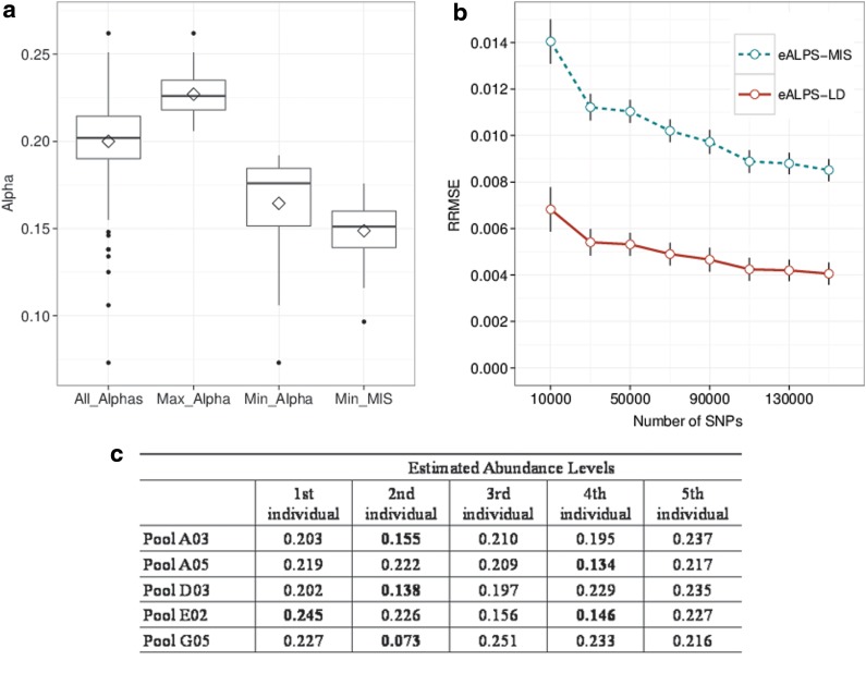
In the NHL data, we have 31 pools in which the genotype information for all individuals is available. For these pools, approximately 150,000 SNPs (depending on the specific pool) were both genotyped then sequenced in the pooled study and finally passed the quality control step in ELAND. Figure 2 illustrates how some pools contain individuals with relative abundances that are significantly higher (or lower) compared to other individuals in that pool. This result demonstrates how the process of preparing DNA pools with specific fractions of DNA from each sample can be highly inaccurate, which can be explained by the accuracy of laboratory equipment, or by variation of the coverage achieved in the different individuals contained in the sample. Whatever the reason might be, it is clear that performing any analysis (i.e. association study) on these pools requires careful consideration.

FIG. 2.

Relative abundances in individuals from the NHL study, estimated using eALPS, eALPS-LD, and eALPS-MIS. All pools contain five individuals and were intended to have uniform relative abundances. Panel (a) summarizes the distribution of alphas estimate using eALPS on the NHL data, demonstrating that in practice relative abundances vary. The blue boxplots are (from left to right): all relative abundances, the maximal and minimal abundances for every pool, estimates using eALPS. The red boxplot is the minimal relative abundance estimated by eALPS-MIS, showing that the method systematically underestimates the relative abundance of the missing genotype (minimal values were always achieved for the missing individual). Panel (b) compares the error on the NHL data with one masked genotype as a function of the number of SNPs used in the analysis. The error rates were calculated with respect to the estimated abundance levels obtained from the eALPs method that was given the full genotype data. Panel (c) shows pools with extreme relative abundances. NHP, non-Hodgkins's lymphona.

3.3.2. Missing genotypes

To assess the accuracy of the missing genotype methods on real data, we masked one genotype of each individual from each of a set of 14 pools, and we ran both eALPS-MIS and eALPS-LD. Figure 2a and 2b presents the results for these experiments, where eALPS is used as a baseline for the calculation of RMSE. As can be clearly observed from Figure 2b, eALPS-LD outperforms eALPS-MIS. Moreover, eALPS-MIS tends to systematically underestimate the relative abundances of the missing individual, which can be explained by the unrealistic uniform prior on possible genotypes. In a sense, incorporating LD is equivalent to applying a very informative position-specific prior on the possible genotypes of the missing individual. The results strongly demonstrate that this approach is highly beneficial.

3.4. Model validation

To evaluate the overall fit of the proposed model to real data, it is natural to ask whether the addition of relative abundance levels is necessary and whether a more complicated model is in place. We therefore perform two likelihood ratio tests—LRT1 and LRT2—using the data obtained from the NHL study. The specifics of the latter test are hereby given in more detail, with LRT1 being carried out along similar lines.

For a given position with the observed minor allele counts x_j, LRT2 considers the eALPS generative model on one hand, with fixed relative abundances α estimated using eALPS, and the unrestricted (saturated) model on the other, allowing the relative abundances to vary across positions. The likelihood for position j under this unrestricted model is given by:

(4)

where A_j is an N-dimensional vector of relative abundances estimated in position j. It is easy to verify that the vector A_j maximizing the above likelihood is given by the solution of . Assuming no positions are homozygous in all N individuals, a solution exists, and we can calculate the maximum likelihood estimate (MLE) under the unrestricted model. 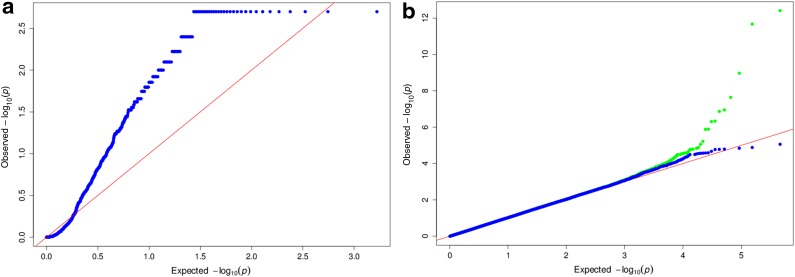For every position, we calculate the likelihood ratio statistic: and obtain the corresponding p-values using a Monte-Carlo simulation of the null distribution. To cancel the effect of genotype errors, we sort the positions in decreasing order of their likelihood ratio statistic, picking only the top (1 − δ)M positions. If the p-values corresponding to these positions are uniformly distributed, then we can state that at least for that subset of positions, the alternative model does not explain the data significantly better than our suggested model (eALPS). This approach was performed on all pools of the NHL data, with the genotyping error probability set to δ = 0.05. Evidently, when this approach is applied to the α estimates obtained by eALPS, we obtain a uniform distribution of p-values, suggesting that the estimates are accurate (Fig. 3).

FIG. 3.

(a) LRT1: Comparing a simple model that assumes uniform relative abundances (the null hypothesis) to eALPS (the alternative hypothesis), using an LRT on every SNP separately. Permutations were performed to obtain p-values that are visualized using a QQ-plot. It is evident that the p-values are systematically smaller than the expected uniform distribution under the null, suggesting that the null hypothesis can be rejected. (b) LRT2: Comparing eALPS (the null hypothesis) to a model that allows relative abundances to vary across positions. The green points are p-values for all positions, and the blue points are the p-values after discarding putative genotype errors according to an error probability of 0.05. In both plots, the x-axis is the – log of p-values drawn from the uniform distribution (uniform quantile), and the y-axis is the – log of the p-values. LRT, likelihood ratio test.

In LRT1, we compare the eALPS model, now in the role of the alternative model, to a simpler model that assumes uniform relative abundances (i.e., α_i = 0.2 for every i). In contrast to the previous test, this time around we obtain a substantial bias from the uniform distribution in the direction of smaller p-values, suggesting that a more complicated model is necessary to explain the data.

3.5. Bacterial community reconstruction

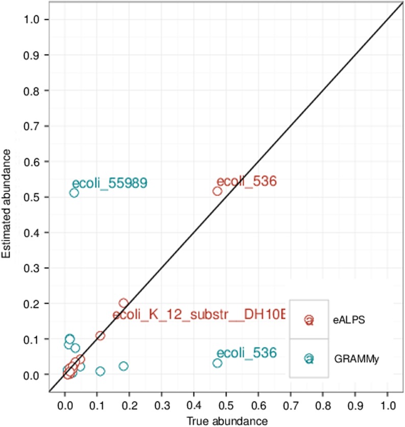
We generated simulated datasets that enable the performance of our method to be assessed. The organisms used as the reference panel were downloaded from the 2012 version of the National Center for Biotechnology Information (NCBI) RefSeq database (Pruitt et al., 2012), that provides access to over 10,000 microbial sequences and specifically 57 strains of Escherichia coli that were used in our experiments. A table of orthologous gene annotations in these strains was obtained from the microbial genome database for comparative analysis (MGBD) (Uchiyama et al., 2012). The genes were aligned to a single strand of E. coli using BWA (Li and Durbin, 2010), and SNPs were called using the Free-Bayes variant detector (Garrison and Marth, 2012). To simulate random relative abundances, we sample from a uniform distribution and from a power-law distribution. Intuition for the choice of a reasonable distribution of relative abundance levels can be obtained from well-studied rank-abundance curves—that is, the relative abundance drawn as a function of species ordered from the most abundant to the least abundant. For many bacterial communities, for example, bacteria in the human skin (Gao et al., 2007), this curve was shown to follow a power-law distribution. Short reads from a metagenomic sample were simulated using MetaSim (Richter et al., 2008). Figure 4 shows that GRAMMY does not perform well when the bacterial community is homogeneous, while our method is considerably more robust to such scenarios.

FIG. 4.

Comparison of eALPS-BCR with GRAMMy on a simulated dataset of 57 strains of Escherichia coli. The blue and red dots represent the estimated abundance levels produced by eALPS-BCR and GRAMMy, respectively. Evidently, eALPS-BCR produces estimations that are particularly accurate for closely related organisms.

4. Conclusion and Discussions

Utilizing pooling techniques to perform rare-variant GWA studies using HTS data is an increasing trend in the field of human genetics (Price et al., 2010). However, in order to avoid spurious associations one must acquire good estimates of the true abundances of individuals in each pool. In this work we propose a statistical model that computes the abundance levels of each individual, incorporating sequencing error. Our model takes advantage of the fact that genotype data of each individual is given, and we extend it to the case in which one or more individual genotype data are missing from the study. We validated our model both of simulated and real data obtained from a non-Hodgkin's lymphoma study, showing that accurate estimates of relative abundance levels can be achieved under low-coverage conditions and that accuracy in datasets with missing data can be brought to a comparable level using LD structure learned from a population reference panel.

Although the problem of relative abundance levels estimation in pooled studies, being a convex optimization problem (see Appendix Section), is far from computationally intensive, a short discussion of running time is still in place. For the case of no missing genotype data, the running time of eALPS for one pool, on a single machine using one CPU, was around 1 hour. Estimation in the presence of missing genotypes poses more computational burden, as all possible genotypes are iterated in every E-step of the algorithm. For a single missing genotype, this only increases the complexity by a factor of 3, but for several missing genotypes complexity will grow exponentially in the number of missing genotypes. More importantly, running time is influenced by the convergence properties of the expectation-maximization algorithm. In our simulations, we observed that incorporating LD greatly improves the speed of convergence, bringing running time of the eALPS-LD method to a few hours on a single machine rather than several days for the eALPS-MIS method.

We illustrated that our method is applicable to the bacterial reconstruction problem, where a mixture of bacteria is given, and the goal is to detect the bacteria existing in the sample and the fraction of it, and show that it outperforms the state-of-the-art method when applied to a simulated dataset of closely related E-coli strands. The eALPS-BCR model currently assumes that sequence reads can be mapped to a unique reference genome and are otherwise discarded from further analysis. This assumption is clearly overoptimistic in realistic metagenomic scenarios, and we therefore plan to extend this framework so as to incorporate read-mapping ambiguity. Another limitation of the current model is the requirement that all reference sequences share a sufficient number of homologous regions that are used in the variant-calling procedure. This was shown in the Results section to be very efficient when the sample consists of only closely related bacteria but will naturally fail when a more diverse sample is used. It will therefore be necessary to combine this prototype with a standard similarity-based method that considers reads mapped to nonhomologous regions. Such a hybrid method is expected to perform well on various metagenomic datasets, and it would then be appropriate to apply it to publicly available complex microbiomes such as the FAMeS dataset, specifically designed for comparison of metagenomic binning methods.

5. Appendix

5.1. Derivation of the EM algorithm

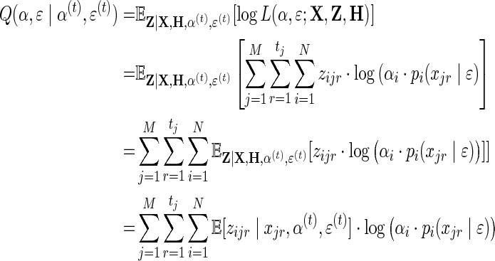
The Q-function is:

(5)

Denote:

(6)

Then we have:

(7)

Applying Gibbs' inequality in (7), the update step for α is:

(8)

Where the probability of observing g_ij given the true allele counts h_ij is (for 1 ≤ i ≤ N′):

and:

Note that if we assume a uniform prior on g_ij and h_ij, the probability of having a true allele count h_ij given the observed genotype g_ij is p(h_ij|g_ij) = p(g_ij|h_ij).

5.2. Missing Genotypes

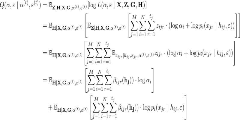
The Q-function is:

(9)

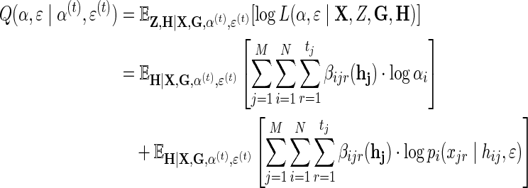
And the Q-function becomes:

(10)

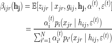
Where:

The second term in the Q-function:

(11)

Maximizing the Q-function with regard to α, and adding the shorthand notations: and we get:

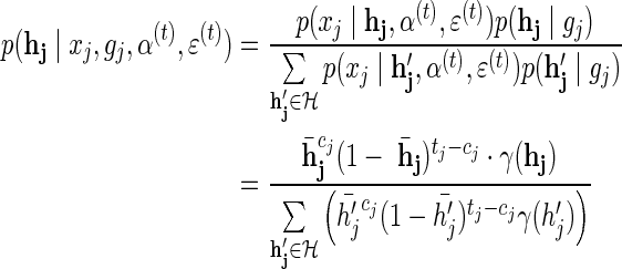Finally, applying Gibbs' inequality in (11), the update step for α_i, 1 ≤ i ≤ N is given by:

maximizing with regard to ɛ involves only the third term in (9), which We solve using a grid search approach.

(12)

5.3. Concavity of the log-likelihood function

In the Methods section we presented the log-likelihood function corresponding to the statistical model assumed by the eALPS framework and described the expectation-maximization scheme used by the eALPS algorithm to find the parameters α and ɛ maximizing it. In this Appendix, we show that the log-likelihood function is in fact concave, implying that the expectation-maximization algorithm is guaranteed to converge to the optimal solution. We begin by showing that the optimization problem involving only the α parameters, while fixing ɛ to be a known constant, is concave. Namely, we would like to show that the function:

(13)

is concave. For this purpose, we write the first- and second-order partial derivatives of f:

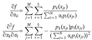(14)

where 1 ≤ k,l ≤ N. The Hessian matrix is therefore:

(15)

where . To verify that ∇ ²f (α) 0 we must show that for every vector v, v^T ∇ ²f (α)v ≤ 0, that is,

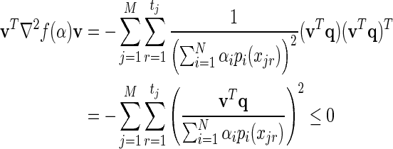(16)

and it follows that f (α) is concave. We now consider the full optimization problem over α and ɛ, for which the log-likelihood becomes:

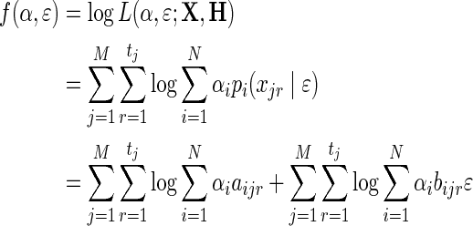(17)

We rewrote p_i(x_jr|ɛ) in 17 as p_i(x_jr|ɛ) = a_ijr + b_ijr, where:

(18)

The first term in (17) is identical to f (α) and is therefore concave using similar arguments just presented for the optimization problem involving only the mixing parameters α. It remains to be shown that the second term is also concave. To do so, we observe that the second term in (17) is:

(19)

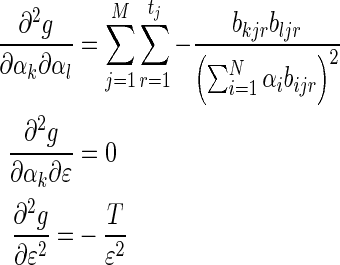
Where is the total number of reads. The partial derivatives of g are therefore:

(20)

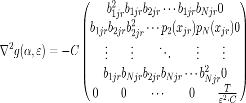
Finally, the Hessian of g(α, ɛ) is a block-diagonal matrix with the structure:

(21)

where 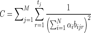. The top-left N × N block was already shown to be positive semi-definite, and is clearly positive semi-definite as well, therefore, the Hessian matrix ∇ ²g(α,ɛ) is negative semi-definite, and we conclude that the optimization problem involving both the mixing parameters α and the sequencing error rate ɛ is concave.

Acknowledgments

I.E., F.H., L.C., J.R., C.S., and E.H. were partially supported by the National Institutes of Health (NIH) grant number 1R01CA154643-01A1. The genotype data was also generated as part of (NIH) grant number 1R01CA154643-01A1. F.E. and E.E. were also supported by National Science Foundation (NSF) grants 0513612, 0731455, 0729049, 0916676, and 1065276, and NIH grants HL080079 and DA024417. I.E. and E.H. were also supported by the German-Israeli Foundation (GIF) grant number 1094-33.2/2010, by the Israeli Science Foundation (grant 04514831), and by the Edmond J. Safra Center for Bioinformatics at Tel-Aviv University. E.H. is a faculty fellow of the Edmond J. Safra Center for Bioinformatics at Tel-Aviv University.

Author Disclosure Statement

No competing financial interests exist.

References

- Amir A. Zuk O. Bacterial community reconstruction using compressed sensing. J. Comp. Biol. 2011;18:1723–1741. doi: 10.1089/cmb.2011.0189. [DOI] [PubMed] [Google Scholar]
- Angly F.E. Willner D. Prieto-Davó A., et al. The GAAS metagenomic tool and its estimations of viral and microbial average genome size in four major biomes. PLoS Comp. Biol. 2009;5:e1000593. doi: 10.1371/journal.pcbi.1000593. [DOI] [PMC free article] [PubMed] [Google Scholar]
- Brown K.M. Macgregor S. Montgomery G.W., et al. Common sequence variants on 20q11.22 confer melanoma susceptibility. Nat. Genet. 2008;40:838–840. doi: 10.1038/ng.163. [DOI] [PMC free article] [PubMed] [Google Scholar]
- Browning S.R. Multilocus association mapping using variable-length Markov chains. Am. J. Hum. Genet. 2006;78:903–913. doi: 10.1086/503876. [DOI] [PMC free article] [PubMed] [Google Scholar]
- Conde L. Halperin E. Akers N.K., et al. Genome-wide association study of follicular lymphoma identifies a risk locus at 6p21.32. Nat. Genet. 2010;42:661–664. doi: 10.1038/ng.626. [DOI] [PMC free article] [PubMed] [Google Scholar]
- Coupland P. Chandra T. Quail M., et al. Direct sequencing of small genomes on the Pacific Biosciences RS without library preparation. BioTechniques. 2012;53:365–372. doi: 10.2144/000113962. [DOI] [PMC free article] [PubMed] [Google Scholar]
- Dethlefsen L. Huse S. Sogin M.L. Relman D.A. The pervasive effects of an antibiotic on the human gut microbiota, as revealed by deep 16s rRNA sequencing. PLoS Biol. 2008;6:e280. doi: 10.1371/journal.pbio.0060280. [DOI] [PMC free article] [PubMed] [Google Scholar]
- Erlich Y. Chang K. Gordon A., et al. DNA Sudoku–harnessing high-throughput sequencing for multiplexed specimen analysis. Genome res. 2009;19:1243–1253. doi: 10.1101/gr.092957.109. [DOI] [PMC free article] [PubMed] [Google Scholar]
- Gao Z. hong Tseng C. Pei Z. Blaser M.J. Molecular analysis of human forearm superficial skin bacterial biota. Proc. Natl. Acad. Sci. U.S.A. 2007;104:2927–2932. doi: 10.1073/pnas.0607077104. [DOI] [PMC free article] [PubMed] [Google Scholar]
- Garrison E. Marth G. Haplotype-based variant detection from short-read sequencing. arXiv preprint. 2012 arXiv:1207.3907. [Google Scholar]
- Golan D. Erlich Y. Rosset S. Weighted pooling–practical and cost-effective techniques for pooled high-throughput sequencing. Bioinformatics. 2012;28:i197–i206. doi: 10.1093/bioinformatics/bts208. [DOI] [PMC free article] [PubMed] [Google Scholar]
- Guarner F. Malagelada J.-R. Gut flora in health and disease. Lancet. 2003;361:512–519. doi: 10.1016/S0140-6736(03)12489-0. [DOI] [PubMed] [Google Scholar]
- Gunderson K.L. Steemers F.J. Lee G., et al. A genome-wide scalable SNP genotyping assay using microarray technology. Nat. Genet. 2005;37:549–54. doi: 10.1038/ng1547. [DOI] [PubMed] [Google Scholar]
- Hamady M. Walker J.J. Harris J.K., et al. Error-correcting barcoded primers for pyrosequencing hundreds of samples in multiplex. Nat. Methods. 2008;5:235–237. doi: 10.1038/nmeth.1184. [DOI] [PMC free article] [PubMed] [Google Scholar]
- Hanson R.L. Craig D.W. Millis M.P., et al. Identification of PVT1 as a candidate gene for end-stage renal disease in type 2 diabetes using a pooling-based genome-wide single nucleotide polymorphism association study. Diabetes. 2007;56:975–983. doi: 10.2337/db06-1072. [DOI] [PubMed] [Google Scholar]
- Heselmans M. Reid G. Akkermans L.M.A., et al. Gut flora in health and disease: potential role of probiotics. Curr. Issues Intest. Microbiol. 2005;6:1–7. [PubMed] [Google Scholar]
- Hormozdiari F. Wang Z. Yang W. Eskin E. Efficient genotyping of individuals using overlapping pool sequencing and imputation. Signals, Systems and Computers (ASILOMAR); 2012 Conference Record of the Forty-Sixth Asilomar Conference on Signals, Systems, and Computers; 2012. pp. 1023–1027. [Google Scholar]
- Kennedy J. Mndoiu I. Paaniuc B. Genotype error detection using Hidden Markov Models of haplotype diversity. J. Comp. Biol. 2008;15:1155–1171. doi: 10.1089/cmb.2007.0133. [DOI] [PubMed] [Google Scholar]
- Kimmel G. Shamir R. A block-free hidden Markov model for genotypes and its application to disease association. J. Comp. Biol. 2005;12:1243–1260. doi: 10.1089/cmb.2005.12.1243. [DOI] [PubMed] [Google Scholar]
- Lee J.S. Choi M. Yan X., et al. On optimal pooling designs to identify rare variants through massive resequencing. Genet. Epidemiol. 2011;35:139–147. doi: 10.1002/gepi.20561. [DOI] [PMC free article] [PubMed] [Google Scholar]
- Li H. Durbin R. Fast and accurate long-read alignment with Burrows-Wheeler transform. Bioinformatics. 2010;26:589–595. doi: 10.1093/bioinformatics/btp698. [DOI] [PMC free article] [PubMed] [Google Scholar]
- Lin W.-Y. Zhang B. Yi N., et al. Evaluation of pooled association tests for rare variant identification. BMC Proc. 2011;5(Suppl 9):S118. doi: 10.1186/1753-6561-5-S9-S118. [DOI] [PMC free article] [PubMed] [Google Scholar]
- Mahida Y.R. Microbial-gut interactions in health and disease. Epithelial cell responses. Best Pract. Res. Clin. Gastroenterol. 2004;18:241–253. doi: 10.1016/j.bpg.2003.10.001. [DOI] [PubMed] [Google Scholar]
- Manolio T.A. Brooks L.D. Collins F.S. A HapMap harvest of insights into the genetics of common disease. J. Clin. Invest. 2008;118:1590–1605. doi: 10.1172/JCI34772. [DOI] [PMC free article] [PubMed] [Google Scholar]
- Matsuzaki H. Dong S. Loi H., et al. Genotyping over 100,000 SNPs on a pair of oligonucleotide arrays. Nature Methods. 2004;1:109–111. doi: 10.1038/nmeth718. [DOI] [PubMed] [Google Scholar]
- Neal R.M. Hinton G.E. Learning in Graphical Models. Kluwer Academic Publishers; Dordrecht, The Netherlands: 1998. 1977. A view of the EM algorithm that justifies incremental, sparse, and other variants, 355–368. [Google Scholar]
- Prabhu S. Pe'er I. Overlapping pools for high-throughput targeted resequencing. Genome Res. 2009;19:1254–1261. doi: 10.1101/gr.088559.108. [DOI] [PMC free article] [PubMed] [Google Scholar]
- Price A.L. Kryukov G.V. de Bakker P.I.W., et al. Pooled association tests for rare variants in exon-resequencing studies. Am. J. Hum. Genet. 2010;86:832–838. doi: 10.1016/j.ajhg.2010.04.005. [DOI] [PMC free article] [PubMed] [Google Scholar]
- Pruitt K.D. Tatusova T. Brown G.R. Maglott D.R. NCBI Reference Sequences (RefSeq): current status, new features and genome annotation policy. Nucleic Acids Res. 2012;40:D130–D135. doi: 10.1093/nar/gkr1079. [DOI] [PMC free article] [PubMed] [Google Scholar]
- Richter D.C. Ott F. Auch A.F., et al. MetaSim: a sequencing simulator for genomics and metagenomics. PloS One. 2008;3:e3373. doi: 10.1371/journal.pone.0003373. [DOI] [PMC free article] [PubMed] [Google Scholar]
- Savage D.C. Dubos R. Schaedler R.W. The gastrointestinal epithelium and its autochthonous bacterial flora. J. Exp. Med. 1968;127:67–76. doi: 10.1084/jem.127.1.67. [DOI] [PMC free article] [PubMed] [Google Scholar]
- Skibola C.F. Bracci P.M. Halperin E., et al. Genetic variants at 6p21.33 are associated with susceptibility to follicular lymphoma. Nat. Genet. 2010;41:873–875. doi: 10.1038/ng.419. [DOI] [PMC free article] [PubMed] [Google Scholar]
- Uchiyama I. Mihara M. Nishide H. Chiba H. MBGD update 2013: the microbial genome database for exploring the diversity of microbial world. Nucleic Acids Res. 2012;41:631–635. doi: 10.1093/nar/gks1006. [DOI] [PMC free article] [PubMed] [Google Scholar]
- Wheeler D.a. Srinivasan M. Egholm M., et al. The complete genome of an individual by massively parallel DNA sequencing. Nature. 2008;452:872–876. doi: 10.1038/nature06884. [DOI] [PubMed] [Google Scholar]
- Xia L.C. Cram J.a. Chen T., et al. Accurate genome relative abundance estimation based on shotgun metagenomic reads. PloS one. 2011;6:e27992. doi: 10.1371/journal.pone.0027992. [DOI] [PMC free article] [PubMed] [Google Scholar]