A HIERARCHICAL BAYESIAN MODEL FOR INFERENCE OF COPY NUMBER VARIANTS AND THEIR ASSOCIATION TO GENE EXPRESSION

Abstract

A number of statistical models have been successfully developed for the analysis of high-throughput data from a single source, but few methods are available for integrating data from different sources. Here we focus on integrating gene expression levels with comparative genomic hybridization (CGH) array measurements collected on the same subjects. We specify a measurement error model that relates the gene expression levels to latent copy number states which, in turn, are related to the observed surrogate CGH measurements via a hidden Markov model. We employ selection priors that exploit the dependencies across adjacent copy number states and investigate MCMC stochastic search techniques for posterior inference. Our approach results in a unified modeling framework for simultaneously inferring copy number variants (CNV) and identifying their significant associations with mRNA transcripts abundance. We show performance on simulated data and illustrate an application to data from a genomic study on human cancer cell lines.

1. Introduction

Our understanding of cancer biology and the mechanisms underlying cancer cell growth has progressed tremendously over the past decade. Cancer is the consequence of a dynamic interplay at different molecular levels (DNA, mRNA and protein). Elucidating the association between two or more of these levels would enable the identification of biological relationships that could lead to improvements in cancer diagnosis and treatment. Consequently, studies that integrate different types of high-throughput data are of great interest. This paper is concerned with the integration of gene expression and copy number variant data.

Gene expression levels correspond to the relative abundance of mRNA transcripts. These expression levels can be altered by chromosomal aberrations, such as copy number variants (CNV). CNVs are variations in the copy number of DNA segments due to cytogenetic events, in which the DNA replication process is disrupted and the DNA segment is either replicated (once or several times) or deleted in newly generated cells, leading to local chromosomal amplifications/deletions (Sebat et al. (2004)). Several experimental techniques are available for CNV detection. The most widely used high-throughput technologies include comparative genomic hybridization (CGH) arrays and single nucleotide polymorphism (SNP) arrays. In this paper, we focus on the former, which generates data as reads on thousands or millions of genomic hybridization targets (probes) spotted on a glass surface. Regions of relative gains or losses are identified by measuring the fluorescence ratio of differentially labeled test and reference DNA samples hybridized onto the array. The reference DNA is assumed to have two copies of each chromosome. If the test sample has no copy number aberrations the log₂ of the intensity ratio is theoretically equal to zero.

A number of statistical methods have been developed to infer CNVs from high-throughput array-based technologies. The most widely used rely on hidden Markov models (HMM) (Colella et al. (2007); Wang et al. (2007)) and circular binary segmentation (Venkatraman and Olshen (2007)). Other methods based on clustering have been proposed, including a combination of segmentation and model-based clustering (Picard et al. (2007)) and a Bayesian hierarchical mixture model (Cardin et al. (2011)). These methods process each sample one at a time and require postprocessing of the inferred CNV calls to resolve CNV boundary variations.

In addition to CNV detection, there is often interest in identifying variants associated with specific phenotypes or biological functions. Most of the available methods either directly use the normalized continuous intensity measurements without inferring copy numbers or use the estimated copy numbers as true states, then assess the associations using univariate tests or by performing simple linear regression models with multiple testing correction (Stranger et al. (2007), Wang et al. (2007)). When using the raw measurements, the aggregation of a large number of tests with low p-values in close genetic proximity is considered evidence of copy number-phenotype association. Although this approach has the advantage of circumventing the need to infer copy number, the high noise in the signal intensities leads to the identification of a large number of false positives (Breheny et al. (2012)). On the other hand, using the copy number calls as if they were the true states ignores the uncertainty in the estimation process and can inroduce bias. Several methods have been proposed to incorporate the uncertainty in copy number estimation into the association tests (Barnes et al. (2008), Subirana et al. (2011)).

In the past few years, there has been a growing interest in relating gene expression and CNV data. Indeed, locating CNVs that affect gene dosage is an important step in understanding biological processes underlying various diseases. In cancer, for example, where chromosomal aberrations are widespread due to genomic instability, discovering amplification of oncogenes or deletion of tumor suppressors are important steps in elucidating tumorigenesis. Earlier attempts in this area have used Pearson correlation coefficients to evaluate associations between raw CGH intensities and gene expression levels mapping to the same genomic region (Bussey et al. (2006), Chin et al. (2006)). Choi et al. (2010) developed a double-layered mixture model to simultaneously estimate copy numbers and evaluate the association between each copy number probability score and the expression level of the corresponding gene. These models perform univariate associations between CNVs and gene expression levels on the same chromosomal region. However, it would be expected that multiple CNVs mapping to different genomic regions may be associated to gene regulation, a mechanism that is part of epistasis, see Cordell (2002).

Several multivariate statistical methods for integrating genomic data sets have been proposed in recent years. Monni and Tadesse (2009) proposed a stochastic partitioning method to identify sets of correlated gene expression levels and select sets of chromosomal abberations that jointly modulate mRNA transcript abundance in the co-expressed genes. Other authors have proposed variable selection methods in multivariate linear regression models in the context of eQTL (expression quantitative trait loci) analysis. Among those, Richardson et al. (2010) proposed mixture priors that enforce sparsity while enhancing the detection of predictors that are associated with many responses. Similar priors have also been studied by Scott-Boyer et al. (2012) for eQTL analysis.

In this paper we develop an innovative statistical model that integrates gene expression and copy number variant data. The proposed approach provides a unified framework to simultaneously infer CNVs across all samples and identify significant associations between copy number states and gene expression changes. To achieve this goal we first specify a joint distribution of the observed gene expression and CGH data across all samples. Using a measurement error model formulation, we factor this joint distribution into the product of conditionally independent submodels: an outcome model that relates the gene expression levels to latent copy number states, and a measurement model that relates these latent states to the observed surrogate CGH measurements using a first order hidden Markov model (HMM). We identify CNVs associated with gene expression changes by incorporating a latent indicator for variable selection into the outcome model and specifying selection priors that account for spatial dependences between adjacent DNA segments. Our strategy for posterior inference uses MCMC algorithms and stochastic search methods and results in the estimation of copy number states across all samples, as well as the selection of groups of CNVs associated with gene expression. The model we propose allows the identification of the joint effect of multiple CNVs on mRNA transcript abundance, rather than assuming univariate associations. In addition, the simultaneous evaluation of multiple gene expression levels reduces the detection of false positive associations by borrowing information across co-expressed genes. We show the performance of our proposed model on simulated data. We also analyze a case study on human cancer cell lines. Findings support the hypothesis that our approach has the potential to discover important linkages between gene expression and cancer.

The rest of the paper is organized as follows: Section 2 introduces the modeling framework and its major components and Section 3 describes the posterior inference and prediction. Results on simulated data are reported in Section 4 while Section 5 is devoted to our case study. Section 6 contains some final remarks.

2. Hierarchical Model

We propose a hierarchical model that integrates gene expression levels with copy number variant data and that accounts for the measurement error in the observed CGH intensities via a hidden Markov model (HMM). The model further incorporates a variable selection procedure and utilizes prior distributions that exploit the dependencies across adjacent DNA segments. Our modeling strategy provides a unified approach for simultaneously inferring copy number states for all samples and identifying associations between sets of copy number variants and gene expression levels. The graphical formulation of the model is illustrated in Figure 1 and its major components are described below. We also summarize the hierarchical formulation of our full model in Figure 2.

Fig 1.

Graphical formulation of the probabilistic model described in Section 2.

Fig 2.

Hierarchical formulation of the proposed probabilistic model.

Let Y_ig denote the expression measurement for gene g (g = 1, …, G) and X_im the observed CGH measurement, i.e., the normalized log₂ ratio, for the m-th CGH probe (m = 1, …, M), in sample i (i = 1, …, n). We assume the M CGH probes ordered according to their chromosomal location and refer to probes m and m+1 as adjacent. In our modeling approach we treat the observed CGH intensities, X_im, as surrogates for unobserved copy number states, which we indicate with ξ_im. Failure to account for the measurement error, by treating the surrogates as the latent copy number states, may lead to biased results. Here we define four copy number states corresponding to:

• ξ_im = 1 for copy number loss (less than two copies of the fragment);

• ξ_im = 2 for copy-neutral state (exactly two copies of the fragment);

• ξ_im = 3 for a single copy gain (exactly three copies of the fragment);

• ξ_im = 4 for multiple copy gains (more than three copies of the fragment).

Let Z = [Y, X] denote the (n × (G + M)) matrix of observed gene expression measurements and let ξ = [ξ₁, · · ·, ξ_M] be the (n × M) matrix of latent copy number states. We consider a nondifferential measurement error, which assumes that, conditional on the latent state ξ, the observed surrogate X contains no additional information on the response Y (Richardson and Gilks (1993)), i.e., f(Y |ξ, X) = f(Y |ξ). The joint distribution of Z can thus be decomposed into conditionally independent submodels, that correspond to an outcome model relating Y to the latent state ξ and a measurement model relating the surrogate X to ξ, as f(Z|ξ) = f(Y |ξ)f(X|ξ). We further assume conditional independence of the gene expression measurements, given the copy number states (that is, Y_i ⊥ Y_j|ξ₁, …, ξ_M) and conditional independence of the CGH measurements, given their states (that is, X_i ⊥ X_j|ξ₁, …, ξ_M) and write

$$f(\mathit{Z}\mid \mathit{\xi })=\prod _{i=1}^n\left\{\prod _{g=1}^{G}f(Y_{ig}\mid {\mathit{\xi }}_i)\prod _{m=1}^{M}f(X_{im}\mid {\xi }_{im})\right\}.$$ (1)

Even though we make these assumptions, we still borrow strength across genes via our hierarchical prior specification, as described in Section 2.3

2.1. Measurement Error Model via HMM

For the outcome model in (1) we follow Monni and Tadesse (2009) and Richardson et al. (2010) who have suggested linear regression models that integrate gene expression levels with genetic data. For gene g we therefore specify a linear regression model of the type

$$Y_{ig}={\mu }_g+{\mathit{\xi }}_i{\mathit{\beta }}_g+{\epsilon }_{ig},i=1,\dots ,n,$$ (2)

for g = 1, …, G and with μ₁, …, μ_G gene-specific intercepts. We also assume ${\epsilon }_{ig}~N(0,{\sigma }_g^2)$ with ${\sigma }_g^2$ a gene specific variance.

We then define the measurement model in (1) in terms of the emission probabilities of a Hidden Markov Model (HMM). CGH data are “state persistent”, meaning that copy number gains or losses at a region are often associated to an increased probability of gains and losses at a neighboring region. Here, we adapt the model proposed by Guha et al. (2008), that uses hidden Markov models with four copy number states. Methods that consider the number of possible states as a random variable, such as those of Fox et al. (2011), Du et al. (2010) and Costa et al. (2013), may be similarly incorporated into our model. Conditional on the latent copy number states, we assume the observed CGH measurements independent and normally distributed, defining the emission distributions of the HMM as

$$X_{im}\mid ({\xi }_{im}=j)\stackrel{\mathit{iid}}{\sim }N({\eta }_j,{\sigma }_j^2),$$ (3)

with η_j and ${\sigma }_j^2$ representing the expected log₂ ratio and the variance of all CGH probes in state j (j = 1, …, 4). The dependence between the states at adjacent probes is captured by a first order Markov model, which assumes that the probability of being in a particular copy number state at chromosomal location m + 1 depends only on the state at location m,

$$P({\xi }_{i(m+1)}\mid {\xi }_{i1},\dots ,{\xi }_{im})=P({\xi }_{i(m+1)}\mid {\xi }_{im})=a_{{\xi }_{im}{\xi }_{i(m+1)}}.$$

with A = (a_hj) forming the matrix of transition probabilities with strictly positive elements (h, j = 1, …, 4). This matrix has a unique stationary distribution π_A. The initial probabilities of being in each of the states at m = 1 are also assumed to be given by π_A.

2.2. Prior Models for Spatial Dependence

For each gene we wish to find a parsimonious set of CGH aberrations that affect the gene expression levels with high confidence. This is equivalent to inferring which elements of the vector β_g in (2) are non-zero, i.e. a classical variable selection problem. The resulting “network” of gene-CGH associations can be encoded by a (G × M) matrix R of binary elements. Specifically, for gene expression g and CGH probe m, the value r_gm = 1 indicates that the corresponding coefficient β_gm is significant, and should therefore be included in the regression model for gene g. Otherwise, r_gm = 0 indicates that the corresponding regression coefficient is zero. Given R, the regression coefficient parameters are then stochastically independent and have the following mixture prior distribution,

$$\pi ({\beta }_{gm}\mid r_{gm},{\sigma }_g^2)=r_{gm}N(0,c_{\beta }^{-1}{\sigma }_g^2)+(1-r_{gm}){\delta }_0({\beta }_{gm}),$$ (4)

with δ₀(·) a point mass at zero and c_β > 0 a hyperparameter to be chosen (see Section 4). The prior model is completed with a Gamma prior on the error precision, ${\sigma }_g^{-2}~G(\frac{\delta }{2},\frac{d}{2})$, and a Normal distribution on the intercepts, ${\mu }_g\mid {\sigma }_g^2~N(0,c_{\mu }^{-1}{\sigma }_g^2)$, with δ, d and c_μ hyperparameters to be chosen.

Priors of type (4) are known as spike-and-slab priors in the Bayesian variable selection literature, see George and McCulloch (1997) for linear regression models and Brown et al. (1998) and Sha et al. (2004) for multivariate models, and have been employed to infer biological networks of high dimensionality, see for example Jones et al. (2005), Richardson et al. (2010) and Stingo et al. (2010). We adopt the formulation of Stingo et al. (2010) which allows to select different covariates (CNV aberrations) for different responses (genes). See also Monni and Tadesse (2009) for an approach based on partition models.

We now describe our prior choice for the elements r_gm’s of this matrix R that encodes the association network. Since contiguous regions of copy number changes correspond to the same DNA aberration, they are more likely to jointly affect the expression level of a gene. Accordingly, in our prior distribution we explicitly assume that the probability of selection at location m depends on the copy number states and the selection of the probes at positions {m − 1, m + 1}. Hence, CNVs located in regions of persistent state aberrations may be more likely to be jointly associated with the expression levels of each gene. We represent this dependent association structure as a conditional mixture prior distribution

$$\pi (r_{gm}\mid r_{g(m-1)},r_{g(m+1)},\mathit{\xi },{\pi }_1)={\gamma }_m[{\pi }_1^{r_{gm}}{(1-{\pi }_1)}^{(1-r_{gm})}]+{\sum }_{j=1}^2{\omega }_m^{(j)}{I}_{\{r_{gm}=r_{g(m+{(-1)}^j)}\}},$$ (5)

where γ_m ∈ [0, 1] and ${\sum }_{j=1}^2{\omega }_m^{(j)}=(1-{\gamma }_m)$. According to (5), with probability γ_m we have that r_gm ~ Bern(π₁), independently of the neighboring values, whereas, with probability (1 − γ_m), r_gm coincides with either one (or both) of the adjacent values in R. We note that equation (5) reduces to the typical independence assumption, r_gm ~ Bern(π₁), in the case γ_m = 1.

In this paper we assume that the parameters γ_m, ${\omega }_m^{(1)}$ and ${\omega }_m^{(2)}$ are probe-specific, capturing information on the physical distance between CGH probes and their unobserved copy number states. More specifically, let d_m be the distance between the adjacent probes {m−1, m} and let D be the total length of the DNA fragment (e.g the length of the chromosome) under consideration. We define

$$1-s_{(m-1)m}=1-\frac{1}{n}\sum _{i=1}^n\frac{e^{\{1-\frac{d_m}{D}\}}-1}{e-1}{I}_{\{{\xi }_{im}={\xi }_{i(m-1)}\}}$$ (6)

to capture the frequency of change points at position m in copy number states across all samples. Similar quantities have been used for example by Wang et al. (2008, 2007) and Marioni et al. (2006) to model spatial dependency in copy number detection. Here, instead, we use them to elicit the association between each gene expression and stretches of CNVs in the following sense. If two CGH probes are physically close state persistence might be more likely and the same association pattern would be expected compared to a situation where the two probes are located farther apart on the genome. Accordingly, we define

$$\begin{array}{cc}& {\gamma }_m=\frac{\alpha }{\alpha +s_{(m-1)m}+s_{m(m+1)}},\\ {\omega }_m^{(1)}=\frac{s_{(m-1)m}}{\alpha +s_{(m-1)m}+s_{m(m+1)}},& {\omega }_m^{(2)}=\frac{s_{m(m+1)}}{\alpha +s_{(m-1)m}+s_{m(m+1)}}\end{array}$$ (7)

with α set to a positive real value. In the applications we set ${\omega }_m^{(1)}$ and ${\omega }_m^{(2)}$ to zero for the first and last chromosomal locations, i.e., m = 1 and m = M. We note that, if s_(m−1)m = s_m(m+1) = 0 equation (5) reduces to the independent case, whereas larger values of either s_(m−1)m or s_m(m+1) imply smaller γ_m and, respectively, larger ${\omega }_m^{(1)}$ or ${\omega }_m^{(2)}$, i.e. stronger spatial dependency. The prior probability of r_gm = 1 therefore increases if r_g(m−1) (or r_g(m+1)) is equal to one and if there are more samples with no change between the copy number states at locations m and m − 1 (or m + 1). Finally, we complete prior (5) by further imposing a Beta hyperprior, π₁ ~ Beta(e, f). Integrating π₁ out we obtain

$$\pi (r_{gm}\mid r_{g(m-1)},r_{g(m+1)},\mathit{\xi })={\gamma }_m\frac{\mathrm{\Gamma }(e+f)\mathrm{\Gamma }(e+r_{gm})\mathrm{\Gamma }(f+1-r_{gm})}{\mathrm{\Gamma }(e+f+1)\mathrm{\Gamma }(e)\mathrm{\Gamma }(f)}+{\sum }_{j=1}^2{\omega }_m^{(j)}{I}_{\{r_{gm}=r_{g(m+{(-1)}^j)}\}}.$$ (8)

It is immediate to show that this prior is proper since it is non negative and has finite support.

As for the prior specification of the HMM of equation (3), we assume independent Dirichlet priors across the rows of the transition matrix A, that is, a_h = (a_h1, a_h2, a_h3, a_h4) ~ Dir(ϕ₁, ϕ₂, ϕ₃, ϕ₄), for h = 1, …, 4. For η_j and ${\sigma }_j^2$ in the emission distributions (3) we follow Guha et al. (2008) and assume ${\eta }_j~N({\delta }_j,{\tau }_j^2)I_{\{{\mathit{low}}_{{\eta }_j}<{\eta }_j<{\mathit{upp}}_{{\eta }_j}\}}$ and ${\sigma }_j^{-2}~\text{Gamma}(b_j,l_j)I_{\{{\sigma }_j^{-2}>{\mathit{upp}}_{{\sigma }_j}\}}$, for j = 1, …, 4. Here low_η1 = − ∞, upp_η4 = ∞, while all other hyperparameters are defined by the user on the base of the platform (see Section 4).

Figure 2 summarizes the full hierarchical formulation of our model.

2.3. Choice of the α Parameter

The parameter α in (7) captures the relative strength of the dependence. In particular, α = 0 implies γ_m = 0 (for m = 1, …, M), whereas α → ∞ leads to γ_m = 1, that is the independent prior. In our applications, we found that a poor choice of α can have undesirable effects on the prior probability. To elucidate this further, let us arbitrarily fix s_(m−1)m = s_m(m+1) = .65. Figure 3 shows plots of the prior probabilities (5) for a grid of values of α in [1, 100], for π₁ = .001 and π₁ = .1. These plots show that strong dependence assumptions, i.e. relatively low values of α, may have a differential effect on the probabilities, at the expense of model sparsity. We notice also that the effect of α is stronger when the probability of success of the Bernoulli prior is lower. We discuss sensitivity to α in the simulation studies below.

Fig 3.

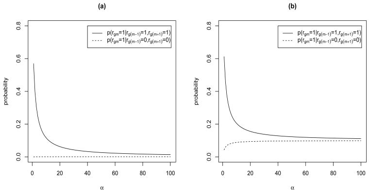
Effect of α on the prior probabilities of inclusion (5) for (a) π₁ = .001 and (b) π₁ = .1.

3. Posterior inference

Our primary interest lies in the estimation of the association matrix R and the matrix of copy number states ξ. Given that the posterior distribution is not available in closed form, we design a Markov chain Monte Carlo algorithm, based on stochastic search variable selection algorithms. Once we integrate out μ, β_g and ${\sigma }_g^2$, the marginal likelihood reduces to

$$f({\mathit{Y}}_g\mid \mathit{\xi },\mathit{R})=\frac{{(2\pi )}^{-\frac{n}{2}}{(\frac{c_{\mu }}{c_{\mu }+n})}^{\frac{1}{2}}{(c_{\beta })}^{\frac{k_g}{2}}\mathrm{\Gamma }(\frac{n+\delta }{2}){(\frac{d}{2})}^{\frac{\delta }{2}}}{{\mid {\mathit{U}}_g\mid }^{\frac{1}{2}}\mathrm{\Gamma }(\frac{\delta }{2}){(\frac{d+q_g}{2})}^{(\frac{n+\delta }{2})}},$$ (9)

where $q_g={\mathit{Y}}_g^{\prime }{\mathit{H}}_n{\mathit{Y}}_g-{\mathit{Y}}_g^{\prime }{\mathit{H}}_n{\mathit{\xi }}_R{\mathit{U}}_g^{-1}{\mathit{\xi }}_R^{\prime }{\mathit{H}}_n{\mathit{Y}}_g,{\mathit{U}}_g=c_{\beta }{\mathbf{I}}_{k_g}+{\mathit{\xi }}_R^{\prime }{\mathit{H}}_n{\mathit{\xi }}_R$ and ${\mathit{H}}_n={\mathbf{I}}_n-\frac{{\mathbf{1}}_n{\mathbf{1}}_n^{\prime }}{n+c_{\mu }}$, with k_g indicating the number of selected regressors for the gth regression function. We give full details of our MCMC algorithm in the supplementary material (Cassese et al. (2013)). The updates at a generic iteration can be described as follows:

• Update R via a Metropolis step. We first select n_g genes at random using a geometric distribution with parameter p_R. Then, for each selected gene, with probability ρ we choose between an Add/Delete or Swap moves; for the Add/Delete move we select at random one of the elements in the corresponding row of R and change its value (from 0 to 1, or viceversa); for the Swap move we select two elements with different inclusion status and swap their values. In updating R, we do not consider CGH probes called in copy neutral state in more than n × p_MC samples at the current MCMC iteration (with p_MC set by the user), since these would not be expected to be associated with changes in mRNA transcript abundance. The proposed move is then accepted with probability

  $$min[\frac{f(\mathit{Y}\mid \mathit{\xi },{\mathit{R}}^{\mathit{new}})\pi ({\mathit{R}}^{\mathit{new}}\mid \mathit{\xi })}{f(\mathit{Y}\mid \mathit{\xi },{\mathit{R}}^{\mathit{old}})\pi ({\mathit{R}}^{\mathit{old}}\mid \mathit{\xi })},1].$$

  Since all moves are symmetric, the proposal distribution does not appear in the previous ratio.

• Update ξ via a Metropolis step. This step consists of choosing at random a column of ξ, say m, and updating the values of n_m of its elements, selected at random using a geometric distribution with parameter p_ξ. For each element, a candidate state is sampled using the current transition matrix A (i.e., we propose ${\xi }_{im}^{\mathit{new}}$ based on ${\xi }_{i(m-1)}^{\mathit{old}}$) and the proposal is accepted with probability

  $$min[\frac{f(\mathit{Y}\mid {\mathit{\xi }}^{\mathit{new}},\mathit{R})f(\mathit{X}\mid {\mathit{\xi }}^{\mathit{new}})\pi (\mathit{R}\mid {\mathit{\xi }}^{\mathit{new}})\pi ({\mathit{\xi }}^{\mathit{new}}\mid {\mathit{\xi }}^{\mathit{old}},\mathit{A})q({\mathit{\xi }}^{\mathit{old}}\mid {\mathit{\xi }}^{\mathit{new}})}{f(\mathit{Y}\mid {\mathit{\xi }}^{\mathit{old}},\mathit{R})f(\mathit{X}\mid {\mathit{\xi }}^{\mathit{old}})\pi (\mathit{R}\mid {\mathit{\xi }}^{\mathit{old}})\pi ({\mathit{\xi }}^{\mathit{old}}\mid {\mathit{\xi }}^{\mathit{old}},\mathit{A})q({\mathit{\xi }}^{\mathit{new}}\mid {\mathit{\xi }}^{\mathit{old}})},1].$$

• Update η_j, for j = 1, …, 4, via a Gibbs step. We sample ${\eta }_j\mid \mathit{X},\mathit{\xi },{\sigma }_j~N({\nu }_j,{\theta }_j^{-2}){\mathbf{I}}_{\{{\mathit{low}}_{{\eta }_j}<{\eta }_j<{\mathit{upp}}_{{\eta }_j}\}}$, with precisions ${\theta }_j={\tau }_j^{-2}+n_j{\sigma }_j^{-2}$ and weighted means ${\nu }_j={\theta }_j^{-2}({\delta }_j{\tau }_j^{-2}+{\overline{X}}_j{n}_j{\sigma }_j^{-2})$, with ${\eta }_j={\sum }_{m=1}^M{\sum }_{i=1}^n{\mathbf{I}}_{\{{\xi }_{im}=j\}}$ and ${\overline{X}}_j=\frac{1}{n_j}{\sum }_{m=1}^M{\sum }_{i=1}^n{X}_{im}{\mathbf{I}}_{\{{\xi }_{im}=j\}}$.

• Update σ_j, for j = 1, …, 4, via a Gibbs step. We sample ${\sigma }_j\mid \mathit{X},\mathit{\xi },{\eta }_j~IG(b_j+\frac{n_j}{2},l_j+\frac{V_j}{2}){\mathbf{I}}_{\{{\sigma }_j^{-2}>{\mathit{upp}}_{{\sigma }_j}\}}$, where ${\eta }_j={\sum }_{m=1}^M{\sum }_{i=1}^n{\mathbf{I}}_{\{{\xi }_{im}=j\}}$ and V_j = (X_im − η_j)²I_{εim=j}.

• Update A via a Metropolis step. We generate a new vector for each row of A as ${\mathit{A}}_{.j}^{\mathit{new}}\mid \mathit{\xi }~\mathit{Dir}({\varphi }_1+o_{h1},{\varphi }_2+o_{h2},{\varphi }_3+o_{h3},{\varphi }_4+o_{h4})$, where $o_{hj}={\sum }_{i=1}^n{\sum }_{m=1}^{M-1}{\mathbf{I}}_{\{{\xi }_{im}=h,{\xi }_{i(m+1)}=j\}}$, and accept it with probability

  $$min[1,\prod _{i=1}^n\frac{{\pi }_{A^{\mathit{new}}}({\xi }_{i1})}{{\pi }_{A^{\mathit{old}}}({\xi }_{i1})}].$$

Given the MCMC output, we first perform inference on R by calculating the marginal posterior probability of inclusion (PPI) for each element, estimated by counting the number of iterations that element was set to 1, after burn-in. A selection is then made by looking at those elements of R that have marginal PPI greater than a value that guarantees an expected rate of false detection (Bayesian FDR) smaller than a fixed threshold, which we set at .05. We follow Newton et al. (2004) and calculate the Bayesian FDR as ${\mathit{FDR}}_B(k)=\frac{{\sum }_g{\sum }_m(1-{\mathit{PPI}}_{gm}){\mathbf{I}}_k}{{\sum }_g{\sum }_m{\mathbf{I}}_k}$, where k is the threshold on the PPI and I_k is an indicator function such that I_k = 1 if (1 − PPI_gm) ≤ k. We then estimate ε by calculating, for each position, the most frequent state value. The MCMC output also allows us to make inference on the HMM parameters, that is, the transition matrix A and the means and variances of the emission distributions in (3).

4. Simulation Studies

We study the performance of our model on a set of simulated scenarios. The normal human genome is diploid. However, recent studies have reported that as much as 12% of the human genome is variable in copy numbers (Redon et al. (2006)). When copy number changes occur, they affect segments of DNA, so neighboring chromosomal regions are expected to have similar copy numbers. Furthermore, transitions from copy number variants to the diploid state are expected to be more likely than transitions between different copy number variants (e.g., from one-copy deletion to one-copy duplication). Taking those considerations into account, we generated a synthetic n × M matrix of copy numbers, ξ, as follows:

• We initialized the matrix ξ with all elements set to 2.

• We randomly selected L < M columns (including some stretches of adjacent columns) and generated their values using the following transition matrix,

  $$\left[\begin{array}{cccc}.7500& .1800& .0500& .020\\ .4955& .0020& .4955& .007\\ .0200& .1800& .7000& .010\\ .0001& .3028& .1000& .597\end{array}\right]$$

• We randomly selected additional $\frac{M-L}{2}$ columns. For each column, we generated 10% of its values according to the transition matrix above.

Following Guha et al. (2008), we sampled the copy number state for the first CGH probe from the initial probability vector π_A, obtained as the normalized left eigenvector associated with the eigenvalue 1. Given the resulting states, we generated the matrix X as in (3), where we fixed η₁ = −.65, η₂ = 0, η₃ = .65, η₄ = 1.5 and σ₁ = .1, σ₂ = .1, σ₃ = .1, σ₄ = .2. We simulated the association network R as follows. First we set all the M − L columns equal to 0. From the remaining columns we selected a total of l elements and set those to 1. We set all the remaining elements to 0. We then generated the regression coefficients corresponding to the l selected associations by sampling from normal distributions, as $\beta ~N({\beta }_0,{\sigma }_0^2)$, where β₀, σ₀ were fixed as detailed in the next sections and the signs were assigned randomly. Finally, we generated the gene expression outcomes, Y_ig (g = 1, …, G) as Y_ig = μ_g + ξ_iβ_g + ε_ig with ${\mu }_g~N(0,{\sigma }_{{\mu }_g}^2)$, σ_μg = .1, and ${\epsilon }_{ig}~N(0,{\sigma }_{\epsilon }^2)$. Unless otherwise specified, in the following we set n = 100, G = 100, M = 1, 000, L = 250, l = 20 and σ_ε = .1. We also considered simulated scenarios with a different σ_ε value for each gene g and found similar performances to those we report below (Cassese et al. (2013)).

As for hyperparameters setting, those in (4) and (5) determine the amount of shrinkage in the model. We followed the guidelines provided by Sha et al. (2004) and chose c_β in the range of variability of the data so as to control the ratio of prior to posterior precision. Specifically, we set c_β = 10, in all simulations. Furthermore, we specified vague priors on the intercept term, by setting c_μ = 10⁻⁶, and on the error variance ${\sigma }_g^2$, by setting δ = 3 and choosing d such that the expected value of ${\sigma }_g^2$ represents a fraction of the observed variance of the standardized responses (5% for the results reported here). For all scenarios, we considered the dependent prior model (8) with e = .001 and f = .999 and assessed sensitivity for varying α in (7) in the set {5, 10, 50, 100, ∞}. The notation α = ∞ succinctly indicates the independent prior. For the HMM model, similarly to Guha et al. (2008), we set ${\eta }_j~N({\delta }_j,{\tau }_j^2)·{\mathbf{I}}_{\{{\mathit{low}}_{{\eta }_j}<{\eta }_j<{\mathit{upp}}_{{\eta }_j}\}},{\sigma }_j^{-2}~Ga(b_j,l_j)·{\mathbf{I}}_{\{\sigma <{\mathit{upp}}_{{\sigma }_j}\}}$ with b_j = 1, l_j = 1, j = 1, …, 4, and the other hyperparameters specified as in Table 1. The lower bound for η₄, low_η4 was set to avoid that a large number of single copy gains be erroneously classified as multiple copy gains. The choice of the truncation ${\sigma }_j^{-2}>6$ is a mild assumption, and it is equivalent to setting σ_j < .41. Finally, we assumed each row of the transition matrix as independently distributed according to Dir(1, 1, 1, 1).

Table 1.

Simulation study: specification of the HMM hyperparameters.

HMM parameters	State 1	State 2	State 3	State 4
δj	−1	0	.58	1
τj	1	1	1	2
lowηj	−∞	−.1	.1	η3 + σ3
uppηj	−.1	.1	.73	∞
uppσj	.41	.41	.41	1

When running the MCMC chains, we sampled initial values for η_j and σ_j from their respective priors, and initialized ξ as ξ_im = j (j = 1, …, 4) if X_im > T_j with T = [−∞, −.5, .29, .79]. We derived the initial value of A from the initial ξ, based on the proportion of transitions. We set the initial R as a matrix with all elements equal to zero. All results reported here were obtained with MCMC chains with 500,000 iterations and a burn-in of 350,000, fixing p_R = .4, p_ξ = .6, p_MC = .9 and ρ = .5. We assessed convergence by inspecting the MCMC sample traces for all parameters, see Figure 4 for an example of typical plots. Moreover, we applied the diagnostic test of Geweke (1992) for the equality of the means, based on the first 10% and the last 50% of the chain. We also used the Heidelberger and Welch (1981) test on the stationarity of the distribution to determine a suitable burn-in.

Fig 4.

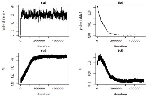
Simulation study: Trace plots for: (a) R, number of ones in the association matrix, (b) ξ₄, number of positions estimated as multiple gains, (c) η₄, mean value of the positions estimated as multiple gains and (d) σ₄, standard deviation of the positions estimated as multiple gains, for one MCMC run on simulated scenario 1. We note that state four has the smallest number of observations, thus more variance and less stationarity is expected.

4.1. Inference on the association network (R)

We present results from two simulated scenarios. The first scenario assumes no particular (spatial) dependence structure in the association between markers and genes. For this scenario, we generated l regression coefficients as β ~ N(2, .3²), except for 6 values which we drew from N(.5, .3²), to take into account a lower signal to noise ratio. In the second scenario we explicitly assumed dependence among the regression coefficients. In particular we selected two clusters of adjacent CGH probes and assumed they affect the expression of the same gene. The corresponding coefficients were sampled as β ~ N(.5, .3²). In both scenarios, we simulated data for two values of the error standard deviation, that is, σ_ε = .1 and σ_ε = .5.

We start by analyzing the results for the first scenario. Figure 5 shows marginal PPIs of the elements r_gm of R, for the case σ_ε = .1. The model recovers well the true gene-CNVs associations (vertical lines), although it is evident that relatively small values of α, implying greater a priori dependence structure, result in an increased number of erroneous decisions when such structure is indeed not present in the data. A selection of the significant associations is made by considering at those elements of R that have marginal PPI greater than a value that guarantees a pre-specified FDR. For example, the first panel of Table 2 reports results in terms of specificity, sensitivity, false positives (FP), false negatives (FN) and number of detections, obtained with an upper bound on the FDR set to .05. Sensitivity is calculated as the ratio of true positive (TP) counts over l and specificity as the ratio of true negatives (TN) over (G×M − l). In the same Table we also report the realised Bayesian q-value, calculated as min_{{(1 − PPI)≤k}} FDR_B(k), see for example Broet et al. (2004) and Morris et al. (2008). Results show that a lower α leads to less FN calls but increased FP counts. However, due to the large number of TNs, such effect translates in much improved sensitivity at the expense of only a minimal decrease in specificity. Results are similar for σ_ε = .5, although, as expected, the model performance improves when the error variance is smaller (see lower panel of each scenario in Table 2).

Fig 5.

Simulated data: Simulated scenario 1 with σ_ε = .1: Marginal posterior probabilities of inclusion of the elements r_gm of the association matrix R. Plots refer to prior model (8) with (a) α = 20, (b) α = 100, (c) α = ∞ (independent prior). Vertical lines indicate the true gene-CNVs associations.

Table 2.

Simulated scenarios 1 and 2: Results on specificity, sensitivity, false positives, false negatives, number of detections and Bayesian q-values, for the dependent prior model (8) and the independent case (α = ∞), obtained for an FDR threshold of .05.

Scenario 1	α = 5	α = 10	α = 20	α = 30	α = 40	α = 50	α = 100	α = ∞
σε = .1
Spec	.99785	.99795	.99999	1	.99999	.99999	1	1
Sens	.95	.95	.9	.95	.9	.9	.9	.8
FP/FN	215/1	205/1	1/2	0/1	1/2	1/2	0/2	0/4
# detect	234	224	19	19	19	19	18	16
q-value	.048679	.046491	.03444	.042294	.045403	.048651	.024107	.024674
σε = .5
Spec	.99999	.99999	.99999	1	1	1	.99999	.99999
Sens	.95	.95	.9	.9	.9	.85	.8	.8
FP/FN	10/1	1/1	1/2	0/2	0/2	0/3	1/4	1/4
# detect	29	20	19	18	18	17	17	17
q-value	.046464	.041118	.049538	.038603	.0428	.026924	.028897	.033866

Scenario 2	α = 5	α = 10	α = 20	α = 30	α = 40	α = 50	α = 100	α = ∞
σε = .1
Spec	.99987	.99998	.99999	.99999	.99999	.99999	.99999	.99999
Sens	.95	.95	.95	.95	.95	.95	.9	.85
FP/FN	13/1	2/1	1/1	1/1	1/1	1/1	1/2	1/3
# detect	32	21	20	20	20	20	19	18
q-value	.045476	.0452311	.031514	.042635	.044119	.046781	.04567	.035927
σε = .5
Spec	.99989	.99994	.99998	.99998	.99998	.99998	.99998	.99998
Sens	.85	.85	.85	.8	.8	.8	.7	.6
FP/FN	11/3	6/3	2/3	2/4	2/4	2/4	2/6	2/8
# detect	28	23	19	18	18	18	16	14
q-value	.04506	.049371	.039412	.041290	.045759	.047261	.047235	.047865

In order to investigate the effect of the threshold on the PPIs on the selection results, in Figure 6(a) we report ROC-type curves displaying FP counts versus FN counts calculated at a grid of equispaced thresholds in the interval [.07, 1]. The plots clearly show that dependent priors obtained for lower values of α generally outperform the independent case, regardless of the threshold.

Fig 6.

Simulated scenario 1(a) and 2(b) with σ_ε = .1: Numbers of FP and FN obtained by considering different thresholds on the marginal probabilities of inclusion of Figure 5. Threshold values are calculated as a grid of equispaced points in the range [.07, 1]. Plots refer to prior model (8) with different values of α.

Our results are confirmed by the second simulated scenario. As expected, dependent priors improve the FP counts, see the last two panels of Table 2, since the spatial dependence in the gene-CNVs association structure is now explicitly taken into account. Indeed, the independent prior shows worse performance, due to its inability to use information gathered from adjacent probes. As in the first simulated scenario, we again notice that lower values of α lead to less FN calls but increased FP counts, see Table 2 and Figure 6(b). As a general guideline regarding the choice of this parameter, our results indicate that moderate values of α give an appropriate compromise between false positives and false negatives. See Section 6 for additional discussion.

4.2. Inference on the CNV states (ξ) and the HMM parameters

We now turn to the inference on the CGH states, encoded by the matrix ξ. Table 3 reports the misclassification counts and corresponding percent rates. In order to compute these summary statistics, for each element we considered the modal state attained at each genomic location over all MCMC iterations (after burn-in). The misclassification rates appear to be consistent over the different values of α and of the error standard deviation σ_ε A close look at the distribution of the misclassifications over the four states showed that most errors occur between adjacent classes (results not shown).

Table 3.

Simulated scenarios 1 and 2: Results on ξ as number of misclassified copy number states, for the dependent prior model (8) and various values of α.

# Miscl (percent)	α = 5	α = 10	α = 20	α = 30	α = 40	α = 50	α = 100	α = ∞
Scenario 1 αε = .1	179 (.179%)	162 (.162%)	78 (.078%)	78 (.078%)	77 (.077%)	74 (.074%)	74 (.074%)	78 (.078%)
Scenario 1 αε = .5	68 (.068%)	71 (.071%)	70 (.07%)	69 (.069%)	76 (.076%)	68 (.068%)	72 (.072%)	73 (.073%)
Scenario 2 αε = .1	51 (.051%)	58 (.058%)	62 (.062%)	53 (.053%)	60 (.06%)	61 (.061%)	60 (.06%)	62 (.062%)
Scenario 2 αε = .5	60 (.06%)	59 (.059%)	60 (.06%)	55 (.055%)	60 (.06%)	53 (.053%)	53 (.053%)	54 (.054%)

Our model allows also to conduct inference on the parameters of the HMM, i.e. the transition matrix A and the means and variances of the emission distributions in model (3). As an example, scenario 1 (σ_ε = .1) using the independent prior gave the following estimates: η̂ = [−0.64963, 0.00044, 0.64936, 1.50717] and σ̂ = [0.10206, 0.09994, 0.10069, 0.21187], which appear to be all very close to the simulated values, with the exception of σ₄ which is slightly overestimated. This is the standard deviation of the amplification state, that collects all copy number gains larger than 1, so some overestimation might be expected. We obtained similar results in all other simulations we considered. As for the transition matrix across CGH states, the estimates appeared close to the truth (result reported in Cassese et al. (2013)).

4.3. Comparison with single stage approaches

We compare the results based on our unified method, which performs simultaneous CNV detection and selection of significant associations, to single stage approaches that focus solely on CNV detection or solely on association analysis using the raw measurements.

Using the CNV detection method of Guha et al. (2008), which analyzes each sample separately, and specifying the same prior settings as our model, there were respectively 2695 and 8349 misclassified CNV calls for the two scenarios with σ_ε = .1 (instead of 78 and 62 as reported for the independent case in Table 3). This result demonstrates that the integration of multiple samples and the joint modeling of gene expression data offer improved estimation of copy number states.

We also looked into the performance of Bayesian variable selection in a regression model where the predictors are the raw continuous CGH measurements, therefore ignoring the inference of the latent copy number states. For the prior on the variable selection indicators, since the copy number states were not estimated, we cannot use prior model (5). Instead, we assumed the independent prior r_gm ~ Bern(π₁) and set π₁ = .001. For σ_ε = .1, using an FRD threshold of .05, we obtained specificity = 1 and sensitivity = .7 in the first simulated scenario and specificity = 1 and sensitivity = .2 in the second scenario. In both cases the performance of the competing model is worse than that of our model with the independent prior (see Table 2). In particular, in the second scenario the model with the dependent prior outperforms both the model with the independent prior and the competing model that uses the raw continuous CGH measurements.

5. Case Study on Human Cancer Cell Lines

We applied our model to the analysis of the NCI-60 cell line panel, which consists of 60 human cancer cell lines derived from a diverse set of tissues (brain, bone marrow, breast, colon, kidney, lung, ovary, prostate and skin). We downloaded the normalized aCGH Agilent 44K data and the Affymetrix HG-U133A RMA gene expressions using CellMiner (discover.nci.nih.gov/cellminer). In the current analysis, we excluded cell line 40 from the dataset, since no gene expression measurements were available in the repository. We imputed the remaining missing values using the k-nearest neighbor algorithm with k = 5.

In performing our analysis we employed pathway-based scores of the gene expression data. This strategy helped us to reduce the dependence between the outcome variables in model (2) and also to achieve a dimension reduction of the model space. Methods that employ pathway-based scores of gene expression data have become quite popular in genomics, see for example Su et al. (2009); Ovacik et al. (2010); Chen et al. (2010); Drier et al. (2013), among others. More precisely, we considered the genes that map to each one of the 186 KEGG pathways, using the software Compadre (see Rodriguez et al. (2012)). Then, for each pathway, we applied principal component analysis (PCA) to the gene expression data and selected the components that explained at least 80% of the variability. This procedure led us to the selection of G = 3195 pathway components, which we used as response variables in model (2). Furthermore, we considered the 1521 CGH probes mapping to chromosome 8 and selected those that showed variability across tissue types via an ANOVA test with multiplicity correction. This resulted in a set of M = 89 CHG predictors.

For model fitting, we used hyperparameter settings similar to those used in the simulation scenarios described in Section 4. We ran 100, 000 iterations with a burn-in of 50,000, setting p_R = .1, p_ξ = .3 and p_MC = .9 in the MH proposals. As suggested by the results of the simulations, we set α to a relatively small value, that is α = 25. For comparisons, we also looked at the case α → ∞ (that is, the independent prior). As in the simulation study, we assessed convergence by inspecting the MCMC sample traces for all parameters. Moreover, we applied the Geweke diagnostic test for the equality of the means and the Heidelberger and Welch test on the stationarity of the distribution to determine a suitable burn-in.

We ranked the marginal PPIs of the elements of R in order to identify the most significant associations. Figure 7(a) shows a heatmap of the pathway-CNV associations with highest PPI for the case α = 25 (roughly the top 100 associations, which correspond to a threshold of .07 on the PPIs). Figure 7(b) shows the same selection for the independent prior. Notice that the latter heatmap is more sparse. In addition, the heatmap for α = 25 shows a stronger tendency to include groups of adjacent CGH probes as significant for the same pathway component, which is coherent with how we built our prior probability model.

Fig 7.

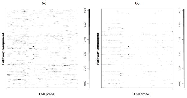
Case study: Heatmaps of PPIs of pathway-CNV associations using the dependent prior with α = 25 (a) and the independent prior (b).

As for inference on the copy number states, the estimates of the state specific means and variances were [−.6419, −.0105, .49, 1.0236] and [.2059, .08115, .1287, .27138], respectively, which are consistent with the theoretical values. Furthermore, the estimated transition matrix well captured the state persistence of the CGHs (results not shown).We also notice that the first and the last value of the vector of estimated variances are larger than those corresponding to neutral and single gain states. This is what we would expect, since the first and the last class correspond to multiple copy number losses and gains, respectively. Finally, Figure 8 shows the estimated frequencies of gains (single and multiple) and losses plotted along the samples for each of the 89 CGH probes considered for analysis.

Fig 8.

Case study: Proportion of estimated gains and losses among the 59 samples for the 89 CGH probes considered.

5.1. Biological interpretation of our findings

Our results identify potential links between genomic mutations, in the form of CNVs, and the transcriptional activity of target pathways. In this Section, we explore the biological significance of the identified associations and assess whether they can be used to generate biologically relevant hypotheses. Figure 9 is a schematic representation of the conceptual relationships between genes linked to CGHs for a set of 4 target pathway components. The 4 pathway components were selected as those with the highest numbers of associations in Figure 7. For each of the 4 components we report the top 20% of the genes with highest PC loadings (subplots A,B,C,D, with bars representing the PC loading values), as those with highest expression variability. Selected genes with CNVs are also listed, below the pathway names. Finally, dashed lines point at genes with CNVs that overlap across selected pathways. These results identify two main molecular pathway blocks. The first (Figure 9A) represents the connection between six genetic mutations with Arginine metabolism. The second (Figure 9BCD) represents a partially overlapping set of 18 genomic mutations and the expression of genes involved in Glycosylphosphatidylinositol (GPI) anchor metabolism and Porphyrin metabolism.

Fig 9.

Case study: Schematic representation of selected associations, showing the selected genes with CNVs and the transcriptional predicted target genes (top 20% of the absolute value of the PC loadings). Bars represent the PC loading values. Dashed lines point at genes with CNVs that overlap across pathways.

There is strong evidence linking Arginine metabolism to cancer in the literature. For example, arginine metyiltransferases are key enzymes in modulating DNA methylation, a primary mechanism in neoplastic transformation (Yang and Bedford (2013)). A connection between Arginine metabolism and suppressor cells in cancer has also been proposed (Raber et al. (2012)). Our results therefore suggest that the expression of a number of enzymes involved in Arginine metabolism may be linked to specific mutations. Interestingly several of these mutations are known cancer genes. For example, it has been shown that mutations in Nucleoplasmin 2 (NPM2), a core histone chaperone involved in chromatin reprogramming, are associated to increase resistance in a cancer cell line (Dalenc et al. (2012)). In the supplementary material (Cassese et al. (2013)) we report details of the functions of other mutations linked to the target pathways we have identified.

Our results also identify a partially overlapping set of mutations linked to GPI-anchor metabolism and Porphyrin metabolism (Figure 9BCD). Similarly to the Arginine metabolism, over-expression of several enzymes in the GPI-anchor metabolism has been shown to induce tumorigenesis and invasion in human breast cancer (Wu et al. (2006)). On the other hand no direct link between the expression of Porphyrin metabolism genes and cancer has been reported, although there is evidence that increased porphyrins may be a parallel disease in liver cancer models (Kaczynski et al. (2009)).

Having identified possible relationships between genomic mutations and target functional pathways we wondered whether these might be also linked to already known regulators involved in cancer. To test this hypothesis, we looked at whether the lists of genes identified either as genetic mutations or target genes are enriched for targets of known regulators. More specifically, we searched for putative (directed or indirect) upstream regulators of all genes involved in the Arginine, GPI-anchor and Porphyrin metabolisms as well as putative upstream regulators of the genes with CNVs selected by the model. We searched a database of known targets of transcription factors and other regulators (www.ingenuity.com) and used a Fisher’s exact test to assess whether there was a statistically significant overlap between the genes in our lists and the genes regulated by each regulator in the database. In this analysis we used a high stringency threshold (p < 10⁻⁶) to define putative regulators. Figure 10 shows our findings. All 4 putative upstream regulators identified at the high stringency threshold were genes known to be of primary importance in cancer biology. These were the well-known oncogenes MYC and p53, the Peroxisome proliferator-activated receptor PPAR (Belfiore et al. (2009)) and the reactive oxygen species scavenger Superoxide dismutase SOD1 (Somwar et al. (2011) and Noor et al. (2002)). We found that genes connected to these regulators were primarily representing enzymes involved in Arginine metabolism (76% of the total targets, 35/46) representing 50% (35/72) of the genes in that pathway. Of these, 6 represented genes within the top 20% PC loadings (Figure 9A). Eight genes connected to the 4 identified regulators (17% of the total targets) were representing enzymes in the Porphyrin metabolism pathway (representing 17% of the total pathway genes, 8/46). Interestingly no genes with CNVs selected in the Arginine metabolism model were linked to the 4 regulators. Instead, 2 of the 3 genes with CNVs included in Figure 10 were in the Porphyrin metabolism pathway block and 1 in the GPI-anchor metabolism. Overall, these findings support the hypothesis that the associations we have identified represent genes highly implicated in cancer.

Fig 10.

Case study: Potential upstream regulators of the selected genes with CNVs and target genes. The plot shows the top 4 most likely regulators (p < 10⁻⁷), that is, PPAR, the oncogenes MYC and p53 and the ROS scavenger SOD1. These are upstream to many of the Arginine metabolism genes (represented by the red circles), including a large number of those in the top 20% of the PC loadings (filled red circles). Some Porphyrin metabolism transcriptional targets are also included (green circles and filled green circles). Furthermore, 3 of the selected genes with CNVs are linked to the 4 regulators (yellow filled green and red circles)

6. Discussion

In this paper we have developed a hierarchical Bayesian modeling framework for the integration of high-throughput data from different sources. We have focused in particular on gene expression levels and CGH array measurements, collected on the same subjects. Our modelling framework has several innovative features. First, it allows the identification of the joint effects of multiple CNVs on mRNA transcript abundance. Second, it reduces the bias that arises when ignoring the uncertainty in the CNV estimation process (i.e. using copy number calls as if they were the true states), by allowing the simultaneous inference of CNVs and their association to gene expression. We have shown in simulations that noise in the raw measurements leads to the detection of spurious associations and also that it is advantageous to incorporate the estimation of copy numbers into the analysis, as this reduces the detection of false positive associations. Findings from an analysis we have conducted on data from 60 cancer cell lines support the hypothesis that the model we have developed has the potential to identify important linkages between gene expression and CNVs. The dataset we have considered spans a large spectrum of tissues and cancer types. It is expected that the detection power of our approach will be higher with more defined patient populations. These studies will require dedicated clinical studies.

Our model aims to identify contiguous regions of DNA aberration that jointly affect the expression of a gene. To accomplish this we have specified selection priors that cleverly account for spatial dependence across DNA segments. This prior model depends on a parameter, α, that plays an important role in capturing the dependence structure. We investigated the option of putting a prior distribution on this parameter. However, with a Gamma prior, for example, and a Metropolis-Hastings step to sample α, the data only have an indirect effect on the MH acceptance ratio, via the definition of s_(m−1)m and the values of r_gm, and the MH ratio is dominated by the prior probability of r_gm. As seen in Figure 3, the prior probability of inclusion/exclusion increases if the neighbors are included/excluded, and this effect is particularly dramatic for the prior probability of inclusion under lower values of α. This causes the sampler to move to regions of the posterior characterized by higher dependence between contiguous states, accepting a move every time a smaller value of α is proposed. Such behavior could be prevented by introducing a second parameter in the prior, in order to penalize for large numbers of included links. The construction of such prior will need further investigation on our part. We find the single-parameter prior model we have proposed here rather intuitive and easy to specify. In our simulations we have found values of α in the range α = [20, 50] to work well, leading to a good balance between the number of FN and FP. Results shown in Table 2, in fact, are clearly robust to the choice of α in this range. Values lower than 20 lead to a steady increase in the number of included links, while values higher than 50 result in priors closer and closer to the independent model. Moreover, for all the simulated examples and all α values in the suggested range, the top 15 links identified with highest posterior probability of inclusion are all true associations. In the case study, as typical with high-throughput genomic data, where there is a high degree of multicollinearity among the covariates, different MCMC runs might pick different subsets of the predictors, as variables that are highly correlated act as proxies for each other and would be picked by different chains. This behavior is, in general, independent of the chosen specification of the α parameter.

In the case study we have applied a heavy filtering of the CGH probes. Filtering and/or dimension reduction methods are often used in applications of HMM models to CGH data, see for instance Du et al. (2010); Fox et al. (2011); Guha et al. (2008); Costa et al. (2013). Caution is necessary when applying such preprocessing steps, as they may result in large gaps between probes, thus decreasing the dependence between adjacent probes and/or inducing heterogeneity in the gap size. In order to assess whether the HMM approach is indeed beneficial we looked at results on the estimation of ξ without the HMM formulation. For this we considered the counts across the four different states as arising from a multinomial distribution and assumed a Dirichlet hyperprior. As we did with the HMM setting, we set all hyperparameters of the Dirichlet to 1. We obtained state specific means [−0.25, −0.03, 0.14, 3.54] and variance estimates [0.41, 0.19, 0.41, 0.78]. The HMM formulation instead resulted in estimated means that were closer to the theoretical values as well as in lower variance estimates (results reported on page 25). In addition, looking at the distributions of the estimated states, the HMM approach resulted in a larger number of neutral states, whereas the no-HMM model classified many of these as single copy number gains. Given the biological evidence that neutral states should be more common, we believe this suggests that the performance of the HMM formulation is superior despite the heavy filtering applied to the data. A possible improvement of our HMM model could be to incorporate the distances between adjacent probes in the evaluation of the transition matrix, to account for possible heterogeneity in the gap size, as done in Colella et al. (2007) and Wang et al. (2007).

Other improvements of our model include the use of indicator variables to model the CNV effects, in order to relax the assumption of a linear association of the ξ categories on the Y s. This would lead to a 2-fold increase (with four categories) in the dimension of the matrix of predictors, therefore increasing computational times. Finally, although we have focused on array CGH data, the proposed method can easily be extended to CNV detection using genome-wide SNP arrays. This can be done by modifying the emission distributions in the HMM and modeling the log-intensity ratios in equation (3) as a mixture of uniform and normal distributions, as in Wang et al. (2007) and Colella et al. (2007).

References

- Barnes C, Plagnol V, Fitzgerald T, Redon R, Marchini J, Clayton D, Hurles ME. A robust statistical method for case-control association testing with copy number variation. Nature Genetics. 2008;40:1245–1252. doi: 10.1038/ng.206. [DOI] [PMC free article] [PubMed] [Google Scholar]
- Belfiore A, Genua M, Malaguarnera R. PPAR-gamma agonists and their effects on IGF-I receptor signaling: Implications for cancer. PPAR Research. 2009 doi: 10.1155/2009/830501. [DOI] [PMC free article] [PubMed] [Google Scholar]
- Breheny Patrick, Chalise Prabhakar, Batzler Anthony, Wang Liewei, Fridley Brooke L. Genetic association studies of copy-number variation: Should assignment of copy number states precede testing? PLoS ONE. 2012;7:e34262. doi: 10.1371/journal.pone.0034262. [DOI] [PMC free article] [PubMed] [Google Scholar]
- Broet P, Lewin A, Richardson S, Dalmasso C, Magdelenat H. A mixture model-based strategy for selecting sets of genes in multiclass response microarray experiments. Bioinformatics. 2004;20:2562–71. doi: 10.1093/bioinformatics/bth285. [DOI] [PubMed] [Google Scholar]
- Brown PJ, Vannucci M, Fearn T. Multivariate Bayesian variable selection and prediction. J of the Royal Statistical Society, Series B. 1998;60:627–641. [Google Scholar]
- Bussey KJ, Chin K, Lababidi S, Reimers M, Reinhold WC, Ku WL, Gwadry F, Kouros-Mehr AH, Fridlyand J, Jain A, Collins C, Nishizuka S, Tonon G, Roschke A, Gehlhaus K, Kirsch I, Scudiero DA, Gray JW, Weinstein JN. Integrating data on DNA copy number with gene expression levels and drug sensitivities in the NCI-60 cell line panel. Molecular Cancer Therapeutics. 2006;5:853–867. doi: 10.1158/1535-7163.MCT-05-0155. [DOI] [PMC free article] [PubMed] [Google Scholar]
- Cardin N, Holmes C, Donnelly P, Marchini J Wellcome Trust Case Control Consortium. Bayesian hierarchical mixture modeling to assign copy number from a targeted CNV array. Genetic Epidemiology. 2011;35:536–548. doi: 10.1002/gepi.20604. [DOI] [PMC free article] [PubMed] [Google Scholar]
- Cassese A, Guindani M, Tadesse MG, Falciani F, Vannucci M. Supplement to ‘A hierarchical Bayesian model for inference of copy number variants and their association to gene expression’. Annals of Applied Statistics. 2013 doi: 10.1214/13-AOAS705. [DOI] [PMC free article] [PubMed] [Google Scholar]
- Chen Xi, Wang Lily, Ishwaran Hemant. An integrative pathway-based clinical-genomic model for cancer survival prediction. Statistics and Probability Letters. 2010;80(17-18):1313–1319. doi: 10.1016/j.spl.2010.04.011. [DOI] [PMC free article] [PubMed] [Google Scholar]
- Chin K, DeVries S, Fridlyand J, Spellman PT, Roydasgupta R, Kuo WL, Lapuk A, Neve RM, Qian Z, Ryder T, Chen F, Feiler H, Tokuyasu T, Kingsley C, Dairkee S, Meng Z, Chew K, Pinkel D, Jain A, Ljung BM, Esserman L, Albertson DG, Waldman FM, Gray JW. Genomic and transcriptional aberrations linked to breast cancer pathophysiologies. Cancer Cell. 2006 Dec;10(6):529–541. doi: 10.1016/j.ccr.2006.10.009. [DOI] [PubMed] [Google Scholar]
- Choi H, Quin ZS, Ghosh D. A double-layered mixture model for the joint analysis of DNA copy number and gene expression data. Journal of Computational Biology. 2010 Feb;17(2):121–137. doi: 10.1089/cmb.2009.0019. [DOI] [PMC free article] [PubMed] [Google Scholar]
- Colella S, Yau C, Taylor JM, Mirza G, Butler H, Clouston P, Bassett AS, Seller A, Holmes CC, Ragoussis J. QuantiSNP: an objective Bayes hidden-Markov model to detect and accurately map copy number variation using SNP genotyping data. Nucleid Acids Research. 2007;35(6):2013–2025. doi: 10.1093/nar/gkm076. [DOI] [PMC free article] [PubMed] [Google Scholar]
- Cordell HJ. Epistasis: what it means, what it doesnt mean, and statistical methods to detect it in humans. Human Molecular Genetics. 2002;11(20):24632468. doi: 10.1093/hmg/11.20.2463. [DOI] [PubMed] [Google Scholar]
- Costa T, Guindani M, Bassetti F, Leisen F, Airoldi EM. Generalized species sampling priors with latent beta reinforcements. 2013. pp. 1–45. arXiv:1012.0866. [DOI] [PMC free article] [PubMed] [Google Scholar]
- Dalenc F, Drouet J, Ader I, Delmas C, Rochaix P, Favre G, Cohen-Jonathan E, Toulas C. Increased expression of a COOH-truncated nucleophosmin resulting from alternative splicing is associated with cellular resistance to ionizing radiation in HeLa cells. Int J Cancer. 2012;100(6):662–668. doi: 10.1002/ijc.10558. [DOI] [PubMed] [Google Scholar]
- Drier Y, Sheffer M, Domany E. Pathway-based personalized analysis of cancer. Proceedings of the National Academy of Sciences. 2013;110(16):6388–6393. doi: 10.1073/pnas.1219651110. [DOI] [PMC free article] [PubMed] [Google Scholar]
- Du L, Chen M, Lucas J, Carlin L. Sticky hidden Markov modelling of comparative genomic hybridization. IEEE TRANSACTIONS ON SIGNAL PROCESSING. 2010;58(10):5353–5368. [Google Scholar]
- Fox E, Sudderth EB, Jordan MI, Willsky AS. A sticky HDP-HMM with application to speaker diarization. Annals of Applied Statistics. 2011;5(2A):1020–1056. [Google Scholar]
- George E, McCulloch RE. Approaches for Bayesian variable selection. Statistica Sinica. 1997;7:339–373. [Google Scholar]
- Geweke J. IN BAYESIAN STATISTICS. University Press; 1992. Evaluating the accuracy of sampling-based approaches to the calculation of posterior moments; pp. 169–193. [Google Scholar]
- Guha S, Li Y, Neuberg D. Bayesian hidden Markov modelling of array cgh data. JASA. 2008;103:485–497. doi: 10.1198/016214507000000923. [DOI] [PMC free article] [PubMed] [Google Scholar]
- Heidelberger Philip, Welch Peter D. A spectral method for confidence interval generation and run length control in simulations. Commun ACM. 1981;24(4):233–245. [Google Scholar]
- Jones B, Carvalho C, Dobra A, Hans C, Carter C, West M. Experiments in stochastic computation for high-dimensional graphical models. Statistical Science. 2005;20(4):388–400. [Google Scholar]
- Kaczynski J, Hansson G, Wallerstedt S. Wallerstedtincreased porphyrins in primary liver cancer mainly reflect a parallel liver disease. Gastroenterology Research and Practice. 2009 doi: 10.1155/2009/402394. [DOI] [PMC free article] [PubMed] [Google Scholar]
- Marioni JC, Thorne NP, Tavare S. BioHMM: a heterogeneous hidden Markov model for segmenting array CGH data. Bioinformatics (Oxford, England) 2006 May;22(9):1144–1146. doi: 10.1093/bioinformatics/btl089. [DOI] [PubMed] [Google Scholar]
- Monni S, Tadesse MG. A stochastic partitioning method to associate high-dimensional responses and covariates. Bayesian Analysis. 2009;4(3):413–436. [Google Scholar]
- Morris JS, Brown PJ, Herrick RC, Baggerly KA, Coombes KR. Bayesian analysis of mass spectrometry proteomic data using wavelet-based functional mixed models. Biometrics. 2008;64(2):479–489. doi: 10.1111/j.1541-0420.2007.00895.x. [DOI] [PMC free article] [PubMed] [Google Scholar]
- Newton MA, Noueiry A, Sarkar D, Ahlquist P. Detecting differential gene expression with a semiparametric hierarchical mixture method. Biostatistics. 2004;5(2):155–176. doi: 10.1093/biostatistics/5.2.155. [DOI] [PubMed] [Google Scholar]
- Noor R, Mittal S, Iqbal J. Superoxide dismutase-applications and relevance to human diseases. Med Sci Monit. 2002;8(9) [PubMed] [Google Scholar]
- Ovacik Meric A, Sukumaran Siddharth, Almon Richard R, DuBois Debra C, Jusko William J, Androulakis Ioannis P. Circadian signatures in rat liver: from gene expression to pathways. BMC Bioinformatics. 2010;11 doi: 10.1186/1471-2105-11-540. [DOI] [PMC free article] [PubMed] [Google Scholar]
- Picard F, Robin S, Lebarbier E, Daudin J. A segmentation-clustering model for the analysis of array CGH data. Biometrics. 2007;63:758–766. doi: 10.1111/j.1541-0420.2006.00729.x. [DOI] [PubMed] [Google Scholar]
- Raber P, Ochoa AC, Rodrguez PC. Metabolism of L-arginine by myeloid-derived suppressor cells in cancer: mechanisms of T cell suppression and therapeutic perspectives. Immunol Invest. 2012;41(6–7):614–634. doi: 10.3109/08820139.2012.680634. [DOI] [PMC free article] [PubMed] [Google Scholar]
- Redon R, Ishikawa S, Fitch KR, Feuk L, Perry GH, Andrews TD, Fiegler H, Shapero MH, Carson AR, Chen W, et al. Global variation in copy number in the human genome. Nature. 2006;444:444–454. doi: 10.1038/nature05329. [DOI] [PMC free article] [PubMed] [Google Scholar]
- Richardson S, Gilks WR. Conditional independence models for epidemiological studies with covariate measurement error. Statistics in Medicine. 1993;12:1703–1722. doi: 10.1002/sim.4780121806. [DOI] [PubMed] [Google Scholar]
- Richardson S, Bottolo L, Rosenthal JS. Bayesian models for sparse regression analysis of high dimensional data. Bayesian Statistics. 2010;9:539–569. [Google Scholar]
- Rodriguez RRR, Duran RCD, Falciani F, Peña JGT, Trevino V. COMPADRE: an R and web resource for pathway activity analysis by component decompositions. Bioinformatics. 2012;28(20):2701–2702. doi: 10.1093/bioinformatics/bts513. [DOI] [PubMed] [Google Scholar]
- Scott-Boyer MP, Imhoolte GC, Tayeb A, Labbe A, Deschepper CF, Gottardo R. An integrated hierarchical Bayesian model for multivariate eQTL mapping. Statistical Applications in Genetics and Molecular Biology. 2012 Jul;11(4):1515–1544. doi: 10.1515/1544-6115.1760. [DOI] [PMC free article] [PubMed] [Google Scholar]
- Sebat J, Lakshmi B, Troge J, Alexander J, Young J, Lundin P, Maner S, Massa H, Walker M, Chi M, et al. Large-scale copy number polymorphism in the human genome. Science. 2004;305:525–528. doi: 10.1126/science.1098918. [DOI] [PubMed] [Google Scholar]
- Sha N, Vannucci M, Tadesse MG, Brown PJ, Dragoni I, Davies N, Roberts TC, Contestabile A, Salmon N, Buckley C, Falciani F. Bayesian variable selection in multinomial probit models to identify molecular signatures of disease stage. Biometrics. 2004;60(3):812–819. doi: 10.1111/j.0006-341X.2004.00233.x. [DOI] [PubMed] [Google Scholar]
- Somwar H, Erdjument-Bromage R, Larsson E, Shum D, Lockwood WW, Yang G, Sander C, Ouerfelli O, Tempst PJ, Djaballah H, Varmus HE. Superoxide dismutase 1 (SOD1) is a target for a small molecule identified in a screen for inhibitors of the growth of lung adenocarci-noma cell lines. PNAS. 2011;108:39. doi: 10.1073/pnas.1113554108. [DOI] [PMC free article] [PubMed] [Google Scholar]
- Stingo FC, Chen YA, Vannucci M, Barrier M, Mirkes PE. A Bayesian graphical modelling approach to microRNA regulatory. Annals of Applied Statistics. 2010;4(4):2024–2048. doi: 10.1214/10-AOAS360. [DOI] [PMC free article] [PubMed] [Google Scholar]
- Stranger BE, Forrest MS, Dunning M, Ingle CE, Beazley C, Thorne N, Redon R, Bird CP, de Grassi A, Lee C, Tyler-Smith C, Carter N, Scherer SW, Tavaré S, Deloukas P, Hurles ME, Dermitzakis ET. Relative impact of nucleotide and copy number variation on gene expression phenotypes. Science. 2007;315:848–853. doi: 10.1126/science.1136678. [DOI] [PMC free article] [PubMed] [Google Scholar]
- Su Junjie, Yoon Byung-Jun, Dougherty Edward R. Accurate and reliable cancer classification based on probabilistic inference of pathway activity. PLoS ONE. 2009;4(12):12. doi: 10.1371/journal.pone.0008161. [DOI] [PMC free article] [PubMed] [Google Scholar]
- Subirana I, Diaz-Uriarte R, Lucas G, Gonzalez JR. CNVassoc: Association analysis of CNV data using R. BMC Med Genomics. 2011;4:47. doi: 10.1186/1755-8794-4-47. [DOI] [PMC free article] [PubMed] [Google Scholar]
- Venkatraman ES, Olshen AB. A faster circular binary segmentation algorithm for the analysis of array CGH data. Bioinformatics. 2007;23:657–663. doi: 10.1093/bioinformatics/btl646. [DOI] [PubMed] [Google Scholar]
- Wang K, Li M, Hadley D, Liu R, Glessner J, Grant SFA, Hakonarson H, Bucan M. Pen-nCNV: an integrated hidden markov model deisigned for high-resolution copy number variation detection in whole-genome SNP genotyping data. Genome Research. 2007;17:1665–1674. doi: 10.1101/gr.6861907. [DOI] [PMC free article] [PubMed] [Google Scholar]
- Wang K, Chen Z, Tadesse MG, Glessner J, Grant SFA, Hakonarson H, Bucan M, Li M. Modeling genetic inheritance of copy number variations. Nucleid Acids Research. 2008;36:21. doi: 10.1093/nar/gkn641. [DOI] [PMC free article] [PubMed] [Google Scholar]
- Wu G, Guo Z, Chatterjee A, Huang X, Rubin E, Wu F, Mambo E, Chang X, Osada M, Sook Kim M, Moon JA, Califano C, Ratovitski EA, Gollin SM, Sukumar S, Sidran-sky D, Trink B. Overexpression of glycosylphosphatidylinositol (GPI) transamidase subunits phosphatidylinositol glycan class T and/or GPI anchor attachment 1 induces tumorigenesis and contributes to invasion in human breast cancer. Cancer Res. 2006;66(20):9829–36. doi: 10.1158/0008-5472.CAN-06-0506. [DOI] [PubMed] [Google Scholar]
- Yang Y, Bedford MT. Protein arginine methyltransferases and cancer. Nat Rev Cancer. 2013;13(1):37–50. doi: 10.1038/nrc3409. [DOI] [PubMed] [Google Scholar]
Associated Data
This section collects any data citations, data availability statements, or supplementary materials included in this article.